Estimation of the charge carrier localization length from Gaussian fluctuations in the magneto-thermopower of $La_{0.6}Y_{0.1}Ca_{0.3}MnO_{3}$

Abstract

The magneto-thermoelectric power (TEP) $\Delta S(T,H)$ of perovskite type manganise oxide $La_{0.6}Y_{0.1}Ca_{0.3}MnO_{3}$ is found to exhibit a sharp peak at some temperature $T^{*}=170K$. By approximating the true shape of the measured magneto-TEP in the vicinity of $T^{*}$ by a linear triangle of the form $\Delta S(T,H)\simeq S_{p}(H)\pm B^{\pm}(H)(T^{*}-T)$, we observe that $B^{-}(H)\simeq 2B^{+}(H)$. We adopt the electron localization scenario and introduce a Ginzburg-Landau (GL) type theory which incorporates the two concurrent phase transitions, viz., the paramagnetic-ferromagnetic transition at the Curie point $T_{C}$ and the ”metal-insulator” (M-I) transition at $T_{MI}$. The latter is characterized by the divergence of the field-dependent charge carrier localization length $\xi(T,H)$ at some characteristic field $H_{0}$. Calculating the average and fluctuation contributions to the total magnetization and the transport entropy related magneto-TEP $\Delta S(T,H)$ within the GL theory, we obtain a simple relationship between $T^{*}$ and the above two critical temperatures ($T_{C}$ and $T_{MI}$). The observed slope ratio $B^{-}(H)/B^{+}(H)$ is found to be governed by the competition between the electron-spin exchange $JS$ and the induced magnetic energy $M_{s}H_{0}$. The comparison of our data with the model predictions produce $T_{C}=195K$, $JS=40meV$, $M_{0}=0.4M_{s}$, $\xi_{0}=10\AA$, and $n_{e}/n_{i}=2/3$ for the estimates of the Curie temperature, the exchange coupling constant, the critical magnetization, the localization length, and the free-to-localized carrier number density ratio, respectively.

I Introduction

The intriguing magnetotransport properties of manganite’s family $R_{1-x}A_{x}MnO_{3}$ (where $R=La,Y,Nd,Pr$ and $A=Ca,Sr,Ba,Pb$) with a $Mn^{3+}/Mn^{4+}$ mixed valence keep attracting much attention of both experimentalists and theorists. [1, 2, 3, 4, 5, 6, 7, 8, 9, 10, 11, 12, 13, 14] In the doping range $0.2<x<0.5$, these compounds are known to undergo a double phase transition from paramagnetic (PM) insulator (I) to ferromagnetic (FM) metal (M) state characterized by the Curie temperature $T_{C}$ and the charge carrier localization temperature $T_{MI}$, respectively. The so-called giant magnetoresistivity (GMR) exhibits a sharp peak around $T_{MI}$, while below $T_{C}$ the system acquires a spontaneous magnetization accompanied by a giant magnetic entropy changes. [14] Despite a variety of theoretical scenarios attempting to describe this phenomenon, practically all of them adopt as a starting point the so-called double-exchange (DE) mechanism, which considers the exchange of electrons between neighboring $Mn^{3+}/Mn^{4+}$ sites with strong on-site Hund’s coupling. The estimated exchange energy [11] $JS=45meV$ (where $S=2$ is an effective spin on a $Mn$ site), being much less than the Fermi energy $E_{F}$ in these materials (typically, $E_{F}=0.15eV$), favors an FM ground state. In turn, an applied magnetic field $H$ enhances the FM order thus reducing the spin scattering and producing the observed negative GMR. The localization scenario, [13] in which $Mn$ oxides are modelled as systems with both DE off-diagonal spin disorder and nonmagnetic diagonal disorder, predicts a divergence of the electronic localization length $\xi(M)$ at some M-I phase transition. In terms of the spontaneous magnetization $M$, it means that for $M<M_{0}$ the system is in a highly resistive (insulator-like) phase, while for $M>M_{0}$ the system is in a low resistive (metallic-like) state. Within this scenario, the Curie point $T_{C}$ is defined through the spontaneous magnetization $M$ as $M(T_{C},H)=0$, while the M-I transition temperature $T_{MI}$ is such that $M(T_{MI},H)=M_{0}$ (with $M_{0}$ being a fraction of the saturated magnetization $M_{s}$). Furthermore, the influence of magnetic fluctuations on electron-spin scattering near $T_{MI}$ is expected to be rather important, for they can easily tip a subtle balance between magnetic and electronic processes in favor of either charge localization or delocalization. Besides, the observable difference between the two critical temperatures (usually attributed to the quality of a particular sample used [5, 6, 7, 8]) is ascribed to the random nonmagnetic scattering which is highly responsible for the magnitude of the observable GMR. [13]

On the other hand, in view of its carrier charge (and density) sensitive nature, thermopower (TEP) measurements could complement the traditional MR data and be used as a tool for probing the field-induced delocalization of the carriers. Indeed, studying the observable magneto-TEP $\Delta S(T,H)=S(T,H)-S(T,0)$ has already proved to be useful for providing important insights into different aspects of high-$T_{c}$ superconductors in the mixed state. [15, 16, 17] Besides, magneto-TEP can be directly linked to the transport entropy change in applied magnetic field. The recently observed [14] giant magnetic entropy change in manganites (produced by the abrupt reduction of the magnetization and attributed to an anomalous thermal expansion just at the Curie point) gives another reason to utilize the magneto-TEP data in order to get an additional information as for the underlying transport mechanisms in these materials.

In the present paper we discuss some typical results for magneto-TEP measurements on a manganite sample $La_{0.6}Y_{0.1}Ca_{0.3}MnO_{3}$ at $H=1T$ field for a wide temperature interval (ranging from $20K$ to $300K$). By approximating the true shape of the measured magneto-TEP in the vicinity of the peak temperature $T^{*}$ by a linear triangle of the form $\Delta S(T,H)\simeq S_{p}(H)\pm B^{\pm}(H)(T^{*}-T)$, we observe that $B^{-}(H)\simeq 2B^{+}(H)$. In an attempt to account for the observed behavior of the magneto-TEP, we adopt the main ideas of the microscopic localization theory [13] and construct a phenomenological free energy functional of Ginzburg-Landau (GL) type which describes the magnetic field and temperature behavior of the spontaneous magnetization in the presence of strong localization effects near $T^{*}$. Calculating the background and fluctuation contributions to the total magnetization and the transport entropy-induced magneto-TEP $\Delta S(T,H)$ within the GL theory, we obtain a simple relationship between $T^{*}$ and the above two critical temperatures ($T_{C}$ and $T_{MI}$). We find also that the observed ratio $B^{-}(H)/B^{+}(H)$ asymmetry is governed by a universal parameter $z=JS/M_{s}H_{0}$ where $JS$ is the electron-spin exchange and $M_{s}H_{0}$ is the localization related magnetic energy. By comparing our data with the model predictions, we deduce estimates for some important model parameters such as the Curie point $T_{C}$, the localization length $\xi_{0}$, the critical magnetization $M_{0}\propto H_{0}$, the exchange energy $J$, and the free-to-localized carrier number density ratio $n_{e}/n_{i}$, all in good agreement with the existing microscopic localization theories.

II Experimental results

$La_{0.6}Y_{0.1}Ca_{0.3}MnO_{3}$ samples were prepared from stoichiometric amounts of $La_{2}O_{3}$, $Y_{2}O_{3}$, $CaCO_{3}$, and $MnO_{2}$ powders. The mixture was heated in the air at $800C$ for 12 hours to achieve the decarbonation. Then it was pressed at room temperature under $10^{3}kG/cm^{2}$ to obtain parallelipedic pellets. An annealing and sintering from $1350C$ to $800C$ was made slowly (during 2 days) to preserve the right phase stoichiometry. A small bar (length $l=10mm$, cross section ${\cal S}=4mm^{2}$) was cut from one pellet. The electrical resistivity $\rho(T,H)$ was measured using the conventional four-probe method. To avoid Joule and Peltier effects, a dc current $I=1mA$ was injected (as a one second pulse) successively on both sides of the sample. The voltage drop $V$ across the sample was measured with high accuracy by a $KT256$ nanovoltmeter. The magnetic field $H$ of $1T$ was applied normally to the current. Fig.1 presents the temperature dependence of the magnetoresistance (MR) $\Delta\rho(T,H)=\rho(T,H)-\rho(T,0)$ for a $La_{0.6}Y_{0.1}Ca_{0.3}MnO_{3}$ sample at $H=1T$ field. As is seen, the negative MR $\Delta\rho(T,H)$ shows a peak (dip) at some temperature $T_{0}=160K$ (referred to as $T_{MI}$, in what follows) where the GMR $\Delta\rho(T,H)/\rho(T,0)$ reaches $40\%$. The thermopower (TEP) $S$ was measured using the differential method. [18] In order to generate a heat flow, a small heater film ($R=150\Omega$) was attached to one end of the sample. Two calibrated chromel-constantan thermocouples were used to measure the temperature difference between two points on the sample. The TEP $S(T,H)$ is deduced from the following equation, $S(T,H)=S_{Au}(T)-V_{s}(T,H)/\Delta T$, where $S_{Au}(T)$ is the TEP of the gold wires used to measure the voltage drop $V_{s}$ at the hot junctions of both thermocouples. Fig.2 shows a typical temperature behavior of the deduced magneto-TEP $\Delta S(T,H)=S(T,H)-S(T,0)$ for the same sample (at $H=1T$). Observe that it has an asymmetric $\Lambda$-like shape near some critical temperature $T^{*}>T_{MI}$ where it reaches its field-dependent peak (dip) value $S_{p}(H)$. Approximating the shape of the observed $\Delta S(T,H)$ by the asymmetric linear triangle of the form

$$\Delta S(T,H)\simeq S_{p}(H)\pm B^{\pm}(H)(T^{*}-T),$$ (1)

with positive slopes $B^{-}(H)$ and $B^{+}(H)$ defined for $T<T^{*}$ and $T>T^{*}$, respectively, we find (see Fig.2) that $B^{-}(H)\simeq 2B^{+}(H)$ in the vicinity of $T^{*}$. Now, with all this information in mind, let us proceed to the interpretation of the experimental results.

III Discussion

A The model

Since we are dealing with the magnetic-field induced changes of the TEP, it is reasonable to assume that the observed behavior can be attributed to the corresponding changes of transport magnetic entropy (and thus spontaneous magnetization) in the presence of strong electron-spin exchange and localization effects, near some critical temperature $T^{*}$. Later on, we will establish a simple (linear) relationship between the peak temperature $T^{*}$ and the two critical temperatures $T_{C}$ and $T_{MI}$, responsible respectively for PM-FM and M-I phase transitions. Based on the above considerations, we can write ${\cal F}={\cal F}_{M}-{\cal F}_{e}$ for the balance of magnetic ${\cal F}_{M}$ and electronic ${\cal F}_{e}$ free energies participating in the transport processes under discussion. The observed magnetization $M$ and the magneto-TEP behavior should result from the minimization of ${\cal F}$ (as, for example, is the case in superconductors where ${\cal F}$ measures the difference between the normal and condensate energies [15, 16]). In our case, the above electronic contribution reads ${\cal F}_{e}={\cal M}{\cal H}_{e}=\eta^{2}(n_{e}E_{k}+n_{i}V_{DE})$ and describes a coupling of spontaneous magnetization ${\cal M}=M_{s}\eta^{2}$ (where $\eta$ is the order parameter and $M_{s}$ the saturated magnetization) with (i) an effective DE energy $V_{DE}=-JS$ (where $S$ is an effective spin on a $Mn$ site, and $J$ the exchange coupling constant), and (ii) the electronic (localization) energy $E_{k}(T,H)=\hbar^{2}/2m\xi^{2}(T,H)$ (where $\xi(T,H)$ is the localization length, and $m$ an effective electron mass); $n_{i}$ and $n_{e}$ stand for the number density of localized spins and conduction electrons, respectively. At the same time, the magnetic contribution ${\cal F}_{M}={\cal M}({\cal H}_{eff}-H)=M_{s}\eta^{2}(\gamma\eta^{2}-H)$ includes the effects due to the molecular-field ${\cal H}_{eff}=\gamma{\cal M}/M_{s}$ (where $\gamma=3k_{B}T_{C}/2\mu_{B}S$ is the characteristic magnetic field with $k_{B}$ the Boltzman constant and $\mu_{B}$ the Bohr magneton) and an applied magnetic field $H$. After trivial rearrangements, the above functional ${\cal F}$ can be cast into a familiar GL type form describing the second-order phase transition from PM (insulator) to FM (metal) state near $T^{*}$, namely

$${\cal F}[\eta]=a\eta^{2}+\frac{\beta}{2}\eta^{4}-\zeta\eta^{2}.$$ (2)

Here $\zeta(H)=M_{s}H-n_{i}JS$ is the effective field-dependent chemical potential of quasiparticles; $a(T,H)=\alpha(H)(T-T^{*})$ with $\alpha(H)=n_{e}\hbar^{2}/2m\xi^{2}_{0}(H)T^{*}$; $\beta=2\gamma M_{s}$, and we used the conventional expression $\xi^{2}(T,H)=\xi^{2}_{0}(H)/(1-T/T^{*})$ for the correlation length. Besides, to account for the field-induced localization effects, we assume after Sheng et al. [13] that $\xi_{0}(H)/\xi_{0}(0)=1/(1-H/H_{0})$ with $H_{0}\simeq\gamma\propto M_{0}$.

B Mean value of the magneto-TEP: $\Delta S_{av}(T,H)$

Given our previous experience with high-$T_{c}$ superconductors, we can readily present the observed magneto-TEP in a two-term contribution form [16]

$$\Delta S(T,H)=\Delta S_{av}(T,H)+\Delta S_{fl}(T,H),$$ (3)

where the average term $\Delta S_{av}(T,H)$ is non-zero only below $T^{*}$ while the fluctuation term $\Delta S_{fl}(T,H)$ should contribute to the observable $\Delta S(T,H)$ both above and below $T^{*}$. In what follows, we shall discuss these two contributions separately within a mean-field theory approximation for GMR materials.

As usual, the equilibrium state of such a system is determined from the minimum energy condition $\partial{\cal F}/\partial\eta=0$ which yields for $T<T^{*}$

$$\eta_{0}^{2}=\frac{\alpha(H)(T^{*}-T)+\zeta(H)}{\beta}$$ (4)

Substituting $\eta_{0}$ into Eq.(2) we obtain for the average free energy density

$$\Omega_{av}(T,H)\equiv{\cal F}[\eta_{0}]=-\frac{[\alpha(H)(T^{*}-T)+\zeta(H)]^{2}}{2\beta}$$ (5)

In turn, the magneto-TEP $\Delta S(T,H)$ can be related to the corresponding difference of transport entropies [15, 16, 17] $\Delta\sigma_{av}\equiv-\partial\Delta\Omega_{av}/\partial T$ as $\Delta S_{av}(T,H)=\Delta\sigma_{av}(T,H)/en_{e}$, where $e$ and $n_{e}$ are the charge and the number density of free carriers. Finally the mean value of the magneto-TEP reads (below $T^{*}$)

$$\Delta S_{av}(T,H)=S_{p,av}(H)-B_{av}(H)(T^{*}-T),$$ (6)

with

$$S_{p,av}(H)=-\frac{\alpha(0)\Delta\zeta(H)}{e\beta n_{e}}(1+z),$$ (7)

and

$$B_{av}(H)=\frac{2\alpha(0)\Delta\alpha(H)}{e\beta n_{e}},$$ (8)

where $z=\Delta\alpha(H)\zeta(0)/\alpha(0)\Delta\zeta(H)$ with $\Delta\alpha(H)=\alpha(H)-\alpha(0)$ and $\Delta\zeta(H)=\zeta(H)-\zeta(0)$.

C Mean-field Gaussian fluctuations of the magneto-TEP: $\Delta S_{fl}(T,H)$

The influence of fluctuations (both Gaussian and critical) on transport properties of high-$T_{c}$ superconductors (including TEP, electrical and thermal conductivity) was extensively studied and is very well documented (see, e.g., [19, 20, 21, 22, 23, 24, 25] and further references therein). In particular, it was found that the fluctuation-induced behavior may extend to temperatures more than $10K$ higher than the critical temperature $T_{c}$. As for manganites, the fluctuation effects in these materials appear to be much less explored. [26] Nonetheless, according to the interpretation of the observed magneto-TEP we adopt in the present paper, influence of magnetic fluctuations on electron-spin scattering near $T^{*}$ should be rather important. So, it seems appropriate to take a closer look at the region near $T^{*}$ to discuss the fluctuations of the magneto-TEP $\Delta S_{fl}(T,H)$. Recall that according to the textbook theory of Gaussian fluctuations, [27] the fluctuations of any observable (such as heat capacity, magnetization, etc) which is conjugated to the order parameter $\eta$ can be presented in terms of the statistical average of the fluctuation amplitude $<(\delta\eta)^{2}>$ with $\delta\eta=\eta-\eta_{0}$. Then the TEP above $(+)$ and below $(-)$ the critical point $T^{*}$ have the form of

$$S_{fl}^{\pm}(T,H)=A<(\delta\eta)^{2}>_{\pm}=\frac{A}{Z}\int d\eta(\delta\eta)^{2}e^{-\Sigma[\eta]},$$ (9)

where $Z=\int d\eta e^{-\Sigma[\eta]}$ is the partition function with $\Sigma[\eta]\equiv({\cal F}[\eta]-{\cal F}[\eta_{0}])/k_{B}T$, and $A$ is a coefficient to be defined below. Expanding the free energy density functional ${\cal F}[\eta]$

$${\cal F}[\eta]\approx{\cal F}[\eta_{0}]+\frac{1}{2}\left[\frac{\partial^{2}{\cal F}}{\partial\eta^{2}}\right]_{\eta=\eta_{0}}\!(\delta\eta)^{2},$$ (10)

around the mean value of the order parameter $\eta_{0}$, which is defined as a stable solution of equation $\partial{\cal F}/\partial\eta=0$ we can explicitly calculate the Gaussian integrals. Due to the fact that $\eta_{0}$ is given by Eq.(4) below $T^{*}$ and vanishes at $T\geq T^{*}$, we obtain finally

$$S_{fl}^{-}(T,H)=\frac{Ak_{B}T^{*}}{4\alpha(H)(T^{*}-T)+4\zeta(H)},\qquad T\leq T^{*}$$ (11)

and

$$S_{fl}^{+}(T,H)=\frac{Ak_{B}T^{*}}{2\alpha(H)(T-T^{*})-2\zeta(H)},\qquad T\geq T^{*}$$ (12)

As we shall see below, for the experimental range of parameters under discussion, $\zeta(H)/\alpha(H)\gg|T^{*}-T|$. Hence, with a good accuracy we can linearize Eqs.(11) and (12) and obtain for the fluctuation contribution to the magneto-TEP

$$\Delta S_{fl}^{\pm}(T,H)\simeq S_{p,fl}^{\pm}(H)\pm B_{fl}^{\pm}(H)(T^{*}-T),$$ (13)

where

$$S_{p,fl}^{-}(H)=-\frac{1}{2}S_{p,fl}^{+}(H)=-\frac{Ak_{B}T^{*}\Delta\zeta(H)}{4\zeta^{2}(0)},$$ (14)

and

$$B_{fl}^{-}(H)=-\frac{1}{2}B_{fl}^{+}(H)=-\frac{Ak_{B}T^{*}\Delta\alpha(H)}{4\zeta^{2}(0)}\left(1-\frac{2}{z}\right).$$ (15)

Furthermore, it is quite reasonable to assume that $S_{p}^{-}=S_{p}^{+}\equiv S_{p}$, where the magneto-TEP peak (dip) values are defined as follows, $S_{p}^{-}=S_{p,av}+S_{p,fl}^{-}$ and $S_{p}^{+}=S_{p,fl}^{+}$. The above equations allow us to fix the arbitrary parameter $A$ yielding $A=-4\zeta^{2}(0)\alpha(0)(1+z)/3ek_{B}T^{*}\beta n_{e}$. This in turn leads to the following expressions for the fluctuation contribution to peaks and slopes through their average counterparts (see Eqs.(7) and (8)): $S_{p,fl}^{+}(H)=(2/3)S_{p,av}(H)$, $S_{p,fl}^{-}(H)=-(1/3)S_{p,av}(H)$, $B_{fl}^{-}(H)=-(1/2)B_{av}(H)$, and $B_{fl}^{+}(H)=B_{av}(H)$. Finally, the total contribution to the observable magneto-TEP reads (Cf. Eq.(1))

$$\Delta S(T,H)=S_{p}(H)\pm B^{\pm}(H)(T^{*}-T),$$ (16)

where

$$S_{p}(H)=-\frac{(1+z)E_{k}^{0}}{3eT^{*}}\left(\frac{H}{H_{0}}\right),$$ (17)

$$B^{+}(H)\equiv B_{fl}^{+}(H)=\left(\frac{n_{e}}{n_{i}}\right)\frac{(z-2)E_{k}^{0}}{JST^{*}}S_{p}(H),$$ (18)

and

$$B^{-}(H) \equiv B_{av}(H)+B^{-}_{fl}(H)$$ (19)

$$= \left[\frac{3z}{(z+1)(z-2)}-\frac{1}{2}\right]B^{+}(H).$$ (20)

Here $E_{k}^{0}=\hbar^{2}/2m\xi^{2}_{0}(0)$, and $z=n_{i}JS/M_{s}H_{0}$. Notice that within our model the asymmetry of slopes ratio $B^{-}(H)/B^{+}(H)$ originates from the balance of the exchange $n_{i}JS$ and localization induced magnetic $M_{s}H_{0}$ energies.

D Magnetization and the critical temperatures

Before turning to the comparison of our theoretical findings with the experimental data, let us discuss the critical temperatures which control the magnetic ($T_{C}$) and carrier localization ”metal-insulator” ($T_{MI}$) phase transitions. According to the adopted model, these two temperatures are defined through the spontaneous magnetization $M=M_{av}+M_{fl}^{-}$ as follows: $M(T_{C})=0$ and $M(T_{MI})=M_{0}$. Here $M_{0}\propto H_{0}$ is the critical magnetization at which the zero-temperature localization length $\xi_{0}(H)=\xi_{0}(0)(1-H/H_{0})^{-1}\propto(1-M/M_{0})^{-1}\to\infty$ marking the M-I phase transition. According to Section III, the average magnetization reads $M_{av}(T)\equiv{\cal M}(\eta_{0})=M_{s}\eta_{0}^{2}(T)$, where $M_{s}=n_{i}\mu_{B}$ is the saturated magnetization, and the equilibrium order parameter $\eta_{0}(T)$ is defined by Eq.(4). Now, for the self-consistency of our approach, we need to find the fluctuation contributions to the magnetization as well. Following the lines of the previous Section, we obtain

$$M_{fl}^{-}(T,H)=\frac{Ck_{B}T^{*}}{4\alpha(H)(T^{*}-T)+4\zeta(H)},\qquad T\leq T^{*}$$ (21)

and

$$M_{fl}^{+}(T,H)=\frac{Ck_{B}T^{*}}{2\alpha(H)(T-T^{*})-2\zeta(H)},\qquad T\geq T^{*}$$ (22)

As usual, to fix the constant $C$, we assume that $M(T^{*})=M^{+}(T^{*})$, where $M^{+}=M_{fl}^{+}$ is the magnetization above $T^{*}$. As a result, we obtain $C=-4M_{s}\zeta^{2}/3k_{B}\beta T^{*}$ which leads to the following expression for the total magnetization below $T^{*}$

$$M=M_{av}+M_{fl}^{-}=M_{s}\left(\eta_{0}^{2}-\frac{\zeta^{2}}{3\beta^{2}\eta_{0}^{2}}\right),$$ (23)

with $\zeta$, $\beta$, and $\eta_{0}$ defined earlier. Given the above definitions, the two critical temperatures are related to each other and to the magneto-TEP peak temperature $T^{*}$ within our model as follows

$$T_{MI}=\left(1-\frac{2M_{0}H_{0}}{n_{e}E_{k}^{0}-n_{i}JS}\right)T_{C},$$ (24)

with

$$T_{C}=\left(1+\frac{yn_{i}JS}{n_{e}E_{k}^{0}}\right)T^{*},\qquad y=1-\frac{1}{\sqrt{3}}.$$ (25)

Let us compare now the obtained theoretical expressions with our experimental data on $La_{0.6}Y_{0.1}Ca_{0.3}MnO_{3}$ (see Fig.2). By comparing the ratios $(B^{-}(H)/B^{+}(H))_{exp}$ and $(B^{-}(H)/B^{+}(H))_{th}$, we obtain $z\simeq 3$ for the slopes asymmetry parameter leading to $JS=3\mu_{B}H_{0}$. Then, using Eq.(18), $B_{exp}^{+}$, $T^{*}=170K$, and just obtained $z$, we get $E_{k}^{0}/JS=2.5(n_{i}/n_{e})$ which in turn brings about $T_{C}=195K$ for the Curie temperature (this value falls into the reported range of the FM transition temperatures for this class of manganites [5, 6, 7, 8]). Using this temperature and assuming $S=2$ for an effective Mn spin, we can estimate the value of the exchange energy $J$ (via the mean-field expression for the critical field $H_{0}=3k_{B}T_{C}/2S\mu_{B}$). The result is: $JS=40meV$, which agrees with other reported estimates of this parameter. [11] Besides, from Eq.(23) we immediately get a simple relationship between the two critical temperatures, $T_{MI}/T_{C}=1-4M_{0}/9M_{s}$ which allows us to estimate the critical magnetization $M_{0}$ (related to the localization magnetic field $H_{0}=\mu_{0}M_{0}$). Using $T_{MI}=160K$ (deduced from the GMR data on the same sample as a peak temperature, see Fig.1), we obtain $M_{0}=0.4M_{s}$, in a good agreement with the localization theory prediction. [13] Next, with the above estimates in mind, Eq.(17) yields $\xi_{0}=10\AA$ for the localization length [5, 13] (using a free electron mass $m_{e}$ for $m$). Finally, observing that $JS\simeq k_{B}T_{C}\simeq 0.3E_{k}^{0}$ we obtain $n_{e}/n_{i}=2/3$ for an estimate of the free-to-localized carrier number density ratio which leads to the saturated magnetization $M_{s}=n_{i}\mu_{B}=(3/2)n_{e}\mu_{B}$. It is also worth noting that the found localization energy $E_{k}^{0}$ is of the order of the Fermi energy $E_{F}$, as expected for manganites. [11] To conclude with the estimates, we note that $\zeta(H)T^{*}/\alpha(H)\simeq 1$ which a posteriori justifies the use of the linearized Eq.(13) for the fluctuation region $|1-T/T^{*}|\ll 1$. As is seen in Fig.2, this criterion is well met in our case.

In summary, to account for the observed temperature dependence of the magneto-TEP $\Delta S(T,H)$ in $La_{0.6}Y_{0.1}Ca_{0.3}MnO_{3}$, exhibiting a field-dependent peak at some temperature $T^{*}$ (lying in-between the charge carrier localization temperature $T_{MI}$ where the observed negative magnetoresistivity has a minimum, and magnetic transition temperature $T_{C}$ which marks the occurence of the spontaneous magnetization), we adopted the ideas of the localization model and introduced a free energy functional of Ginzburg-Landau (GL) type describing the phase transition from paramagnetic (insulator) to ferromagnetic (metal) state near $T^{*}$. Calculating both average and fluctuation contributions to the total magnetization and magneto-TEP within the GL theory, we were able to successfully fit the data and estimate some important model parameters (including the metal-insulator $T_{MI}$ and magnetic $T_{C}$ transition temperatures, localization length $\xi_{0}$, electron-spin exchange coupling constant $J$, and the free-to-localized carrier number density ratio $n_{e}/n_{i}$), all in a reasonable agreement with existing microscopic theories. The Gaussian fluctuations both above and below $T^{*}$ are found to substantially contribute to the peak value $S_{p}(H)\equiv\Delta S(T^{*},H)$ of the observed magneto-TEP, amounting to $67\%$ and $33\%$, respectively.

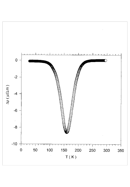
FIG. 1.: The temperature behavior of the observed magnetoresistivity in $La_{0.6}Y_{0.1}Ca_{0.3}MnO_{3}$ at $H=1T$.

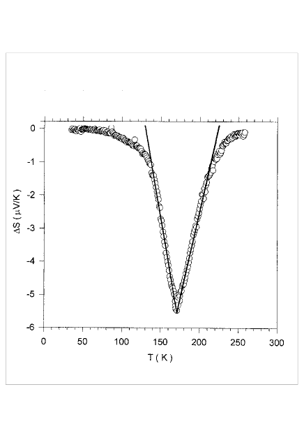
FIG. 2.: The temperature behavior of the observed magneto-TEP in manganite $La_{0.6}Y_{0.1}Ca_{0.3}MnO_{3}$ at $H=1T$. The best fit to the data points according to Eq.(1) yields $S_{p}(H)=-5.49\pm 0.01\mu V/K$, $B^{-}(H)=-0.14\pm 0.01\mu V/K^{2}$, and $B^{+}(H)=-0.08\pm 0.01\mu V/K^{2}$ for the peak and the slopes, respectively.

- [1] H.L. Ju, C. Kwon, Qi Li, R.L. Greene, and T. Venkatesan, Appl. Phys. Lett. 65, 2108 (1994).
- [2] P. Schiffer, A.P. Ramirez, W. Bao, and S.-W. Cheong, Phys. Rev. Lett. 75, 3336 (1995).
- [3] P.G. Radaelli, D.E. Cox, M. Marezio, S.-W. Cheong, P. Schiffer, and A.P. Ramirez, Phys. Rev. Lett. 74, 4488 (1995).
- [4] J. Barrat, M.R. Lees, G. Balakrishnan, and D. McPaul, Appl. Phys. Lett. 68, 424 (1996).
- [5] J. Fontcuberta, M. Martinez, A. Seffar, S. Pinol, J.L. Garcia-Munoz, and X. Obradors, Phys. Rev. Lett. 76, 1122 (1996).
- [6] J.L. Garcia-Munoz, M. Suaaidi, J. Fontcuberta, and J. Rodriguez-Carvajal, Phys. Rev. B 55, 34 (1997).
- [7] J. Fontcuberta, V. Laukhin, and X. Obradors, Appl. Phys. Lett. 72, 2607 (1998).
- [8] J. Fontcuberta, in Nanomagnetic Materials, edited by M. Ausloos and I. Nedkov, to be published in the NATO ASI Series (Kluwer, Dordrecht, 1999).
- [9] A.J. Millis, P.B. Littlewood, and B.I. Shraiman, Phys. Rev. Lett. 74, 5144 (1995); ibid 77, 175 (1996).
- [10] H. Roder, J. Zang, and A.R. Bishop, Phys. Rev. Lett. 76, 1356 (1996).
- [11] W.E. Pickett and D.J. Singh, Phys. Rev. B 53, 1146 (1996).
- [12] C.M. Varma, Phys. Rev. B 54, 7328 (1996).
- [13] L. Sheng, D.Y. Xing, D.N. Sheng, and C.S. Ting, Phys. Rev. Lett. 79, 1710 (1997).
- [14] Z.B. Guo, Y.W. Du, J.S. Zhu, H. Huang, W.P. Ding, and D. Feng, Phys. Rev. Lett. 78, 1142 (1997).
- [15] V. Gridin, S. Sergeenkov, R. Doyle, P. de Villiers, and M. Ausloos, Phys. Rev. B 47, 14594 (1993).
- [16] S. Sergeenkov, V. Gridin, P. de Villiers, and M. Ausloos, Physica Scripta 49, 637 (1994).
- [17] V. Gridin, P. Pernambuco-Wise, C.G. Trendall, W.R. Datars, and J.D. Garrett, Phys. Rev. B 40, 8814 (1989).
- [18] H. Bougrine and M. Ausloos, Rev. Sci. Instrum. 66, 199 (1995).
- [19] M. Ausloos and Ch. Laurent, Phys. Rev. B 37, 611 (1988).
- [20] P. Clippe, Ch. Laurent, S.K. Patapis, and M. Ausloos, Phys. Rev. B 42, 8611 (1990).
- [21] J.L. Cohn, E.F. Skelton, S.A. Wolf, J.Z. Liu, and R.N. Shelton, Phys. Rev. B 45, 13144 (1992).
- [22] M. Houssa, H. Bougrine, S. Stassen, R. Cloots, and M. Ausloos, Phys. Rev. B 54, R6885 (1996).
- [23] M. Houssa, M. Ausloos, R. Cloots, and H. Bougrine, Phys. Rev. B 56, 802 (1997).
- [24] M. Ausloos, S.K. Patapis and P. Clippe, in Physics and Materials Science of High Temperature Superconductors II, edited by R. Kossowsky, B. Raveau, D. Wohlleben, and S.K. Patapis, vol. 209E in the NATO ASI Series (Kluwer, Dordrecht, 1992) pp. 755–785.
- [25] A. A. Varlamov and M. Ausloos, in Fluctuation Phenomena in High Temperature Superconductors, edited by M.Ausloos and A. A. Varlamov, vol. 32 in the NATO ASI Partnership Sub-Series (Kluwer, Dordrecht, 1997), p. 3.
- [26] M. Ausloos, in Magnetic Phase Transitions, edited by M. Ausloos and R.J. Elliot (Springer-Verlag, Berlin, 1983), p. 99.
- [27] H.E. Stanley, Introduction to Phase Transitions and Critical Phenomena, Clarendon Press, Oxford, 1968.