A Lattice Boltzmann Model for Wave and Fracture phenomena

Abstract

We show that the lattice Boltzmann formalism can be used to describe wave propagation in a heterogeneous media, as well as solid-body-like systems and fracture propagation. Several fundamental properties of real fractures (such as propagation speed and transition between rough and smooth crack surfaces) are well captured by our approach.

Lattice Boltzmann (LB) models [1, 2] are dynamical systems, discrete in time and space, aimed at simulating the behavior of a real physical system in terms of local density of fictitious particles moving and interacting on a regular lattice. The density distribution functions are denoted $f_{i}(\vec{r},t)$ where $\vec{r}$ refers to the lattice site, $t$ the iteration time while the subscript $i$ labels the admissible speed of motion $\vec{v}_{i}$ (e.g. along the main lattice directions). The value $i=0$ corresponds to a population of rest particles with $\vec{v}_{0}=0$.

Lattice BGK models [3] have been used successfully to simulate fluid dynamics and complex flows [1, 2]. The same approach can be adapted to model wave propagation in a heterogeneous media, where propagation speed, absorption and reflection can be adjusted locally for each lattice sites. We show how such a model can be derived and applied to the study of fracture propagation

Lattice BGK models are characterized by the following dynamics

$$f_{i}(\vec{r}+\tau\vec{v}_{i},t+\tau)-f_{i}(\vec{r},t)={1\over\xi}\left(f_{i}^{(0)}(\vec{r},t)-f_{i}(\vec{r},t)\right)$$ (1)

where $\tau$ is the time step, $f_{i}^{(0)}(\vec{r},t)$ the so-called local equilibrium distribution and $\xi$ a relaxation time. The function $f_{i}^{(0)}$ is the key ingredient for it actually contains the properties of the physical process under study: this is the distribution to which the dynamics spontaneously relaxes and which is, therefore, intimately related to the nature of the system.

Wave phenomena, whether mechanical or electromagnetic derives from two conserved quantities $\Psi$ and $\vec{J}$, together with time reversal invariance and a linear response of the media. The quantity $\Psi$ is a scalar field and $\vec{J}$ its associated current. For sound waves, $\Psi$ and $\vec{J}$ are respectively the density and the momentum variations. In electrodynamics, $\Psi$ is the energy density and $\vec{J}$ the Poynting vector [4].

The idea behind the LB approach is to “generalize” a physical process to a discrete space and time universe, so that it can be efficiently simulated on a (parallel) computer. For waves, this generalization is obtained by keeping the essential ingredients of real phenomena, namely conservation of $\Psi$ and $\vec{J}$, linearity and time reversal invariance. Thus, in a discrete space-time universe, a generic system leading to wave propagation is obtained from eq. (1) by an appropriate choice of the local equilibrium distribution

$$f_{i}^{(0)}=a\Psi+b{\vec{v}_{i}\cdot\vec{J}\over 2v^{2}}\qquad{\rm if\ }i\neq 0,\ \rm and\ \qquad f_{0}^{(0)}=a_{0}\Psi$$ (2)

where $v$ is the ratio of the lattice spacing to the time step, and $\Psi$ and $\vec{J}$ are related to the $f_{i}$s in the standard way: $\Psi=\sum_{i}f_{i}$ and $\vec{J}=\sum_{i}f_{i}\vec{v}_{i}$. Note that, here, we make no restriction on the sign of the $f_{i}$s which may well be negative in order to represent a wave.

As opposed to hydrodynamics [1], $f_{i}^{(0)}$ is a linear function of the conserved quantities, which ensures the superposition principle. The parameters $a$, $b$ and $a_{0}$ are chosen so that $\Psi=\sum_{i}f_{i}^{(0)}$ and $\vec{J}=\sum_{i}\vec{v}_{i}f_{i}^{(0)}$, which ensures conservation of $\Psi$ and $\vec{J}$. For a two-dimensional square lattice (D2Q5 to use the terminology of [1]) we find $a_{0}+4a=1$ and $b=1$. The freedom on the value of $a_{0}$ can be used to adjust locally the wave propagation speed. Time reversal invariance is enforced by choosing $\xi=1/2$ as can be easily checked from eq. (1) with $\vec{J}\to-\vec{J}$ and $\Psi\to\Psi$ in relation (2). Note that the D2Q5 lattice is known for giving anisotropic contributions to the hydrodynamic equations. These terms are not present in our wave model because they appear with a vanishing coefficient when $\xi=1/2$ (see eq. (LABEL:wave-mvt-2).

In hydrodynamic models, $\xi=1/2$ corresponds to the limit of zero viscosity, which is numerically unstable. In our case, this instability does not show up provided we use an appropriate lattice. Indeed, in the D2Q5 lattice, our dynamics is also unitary [5] which ensures that $\sum_{i}f_{i}^{2}$ is conserved. This extra condition prevents the $f_{i}$s from becoming arbitrarily large (with positive and negative signs, since $\Psi$ is conserved). This is no longer the case with the D2Q9 lattice, where numerical instabilities develop for our wave dynamics. This observation may shed some light on the origin of the numerical instabilities observed in hydrodynamic models.

Note that dissipation can be included in our microdynamics. Using $\xi>1/2$ allows us to describe waves with viscous-like dissipation. This makes sense with the hexagonal lattice D2Q7, where no stability problem occurs when $\xi=1/2$ and no anisotropy problem appears when the viscosity is non-zero ($\xi>1/2$). Below we shall propose another way to include dissipation in the square lattice model, which will be appropriate to our purpose of modeling fracture propagation.

The multiscale Chapman-Enskog expansion [2] can be used to derive the macroscopic behavior of $\Psi$ and $\vec{J}$ when the lattice spacing and time step go to zero. We obtain

$$\partial_{t}\Psi+\partial_{\beta}J_{\beta}=0$$ (3)

$$\partial_{t}J_{\alpha} + 2av^{2}\partial_{\alpha}\Psi+$$ (5)

$$\left(2\xi-1\right)\left[a\tau v^{2}\partial_{\alpha}{\rm div}\vec{J}-{\tau\over 4v^{2}}T_{\alpha\beta\gamma\delta}\partial_{\beta}\partial_{\gamma}J_{\delta}\right]=0$$

where $T_{\alpha\beta\gamma\delta}=\sum_{i}v_{i\alpha}v_{i\beta}v_{i\gamma}v_{i\delta}$ and summation over repeated greek indices (which label the spatial coordinates) is assumed. With $\xi=1/2$ equation (LABEL:wave-mvt-2) becomes $\partial_{t}J_{\alpha}+2av^{2}\partial_{\alpha}\Psi=0$. When combined with equ. (3), we obtain

$$\partial^{2}_{t}\Psi-2av^{2}\nabla^{2}\Psi = 0$$ (7)

which is a wave equation with propagation speed $c=v\sqrt{2a}$ (note that $v$ is the speed at which information travels). As mentioned previously, the propagation speed $c$ can be adjusted from place to place by choosing the spatial dependency of $a$. Provided that $a_{0}+4a=1$ and $a_{0}\geq 0$ (required for stability reasons), the largest possible value is $a=1/4$ and corresponds to a maximum velocity $c_{0}=v/\sqrt{2}$. Therefore media with different refraction indices $n=c_{0}/c=1/(2\sqrt{a})$ can be modeled.

Perfect reflection on obstacles can be included by modifying the microdynamics to be $f_{i}(\vec{r}+\tau\vec{v}_{i},t+\tau)=-f_{i^{\prime}}(\vec{r},t)$ on mirror sites, where $i^{\prime}$ is defined so that $\vec{v}_{i^{\prime}}=-\vec{v}_{i}$, i.e. the flux bounces back to where they came from with a change of sign. Absorption on non-perfect transmitter sites can be obtained by modifying the conservation of $\Psi$ to $\sum_{i}f_{i}^{(0)}=\mu\Psi$, where $0\leq\mu\leq 1$ is an attenuation factor. This modifies $a\to\mu a$ and $a_{0}\to\mu a_{0}$. Finally, by substituting (2) into (1) and using the expression of $a$ and $a_{0}$ in terms of $c$, free propagation with refraction index $n(\vec{r})$, and partial transmission and reflection can be expressed as

$$f_{i}(\vec{r}+\tau\vec{v}_{i},t+\tau) = {\mu\over 2n^{2}}\Psi-f_{i+2}(\vec{r},t)$$ (8)

$$f_{0}(\vec{r},t+\tau) = 2\mu{n^{2}-1\over n^{2}}\Psi-f_{0}(\vec{r},t)$$ (9)

In this equation, $\mu=0$ corresponds to perfect reflection, $\mu=1$ to perfect transmission and $0<\mu<1$ describes a situation where the wave is partially absorbed. A particular version of our LB wave model has been successfully validated by the problem of radio wave propagation in a city [6].

The idea of expressing wave propagation as a discrete formulation of the Huygens principle has been considered by several authors [7, 8, 9, 10]. Not surprisingly, the resulting numerical schemes bear a strong similarity to ours. Nevertheless the context of these studies is different from ours and none have noticed the existing link with the lattice BGK approach. Models of refs. [9, 10] use a reduced set of conserved quantities, which may not be appropriate in our case. Other models [11] consider wave propagation in a LB approach, but with a significantly more complicated microdynamics and a different purpose.

In what follows, we show how our LB dynamics can model a solid body and capture the generic feature of crack propagation. Whereas LB methods have been largely used to simulate systems of point particles which interact locally, modeling a solid body with this approach (i.e modeling an object made of many particles that maintains its shape and coherence over distances much larger than the interparticle spacing) has remained mostly unexplored. A successful attempt to model a one-dimensional solid as a cellular automata is described in [12]. The crucial ingredient of this model is the fact that collective motion is achieved because the “atoms” making up the solid vibrate in a coherent way and produce an overall displacement. This vibration propagates as a wave throughout the solid and reflects at the boundary.

A 2D solid-body can be thought of as a square lattice of particles linked to their nearest neighbors with a spring-like interaction. Generalizing the model given in [12] requires us to consider this solid as made up of two sublattices. We term them black and white, by analogy to the checkerboard decomposition. The dynamics consists in moving the black particles as a function of the positions of their white, motionless neighbors, and vice-versa, at every other steps.

Let us denote the location of a black particle by $\vec{r}_{i,j}=(x_{i,j},y_{i,j})$. The surrounding white particles will be at positions $\vec{r}_{i-1,j}$, $\vec{r}_{i+1,j}$, $\vec{r}_{i,j-1}$ and $\vec{r}_{i,j+1}$. We define the separation to the central black particle as (see figure 1)

$$\vec{f}_{1}(i,j) = \vec{r}_{i,j}-(\vec{r}_{i-1,j}+\vec{h})$$ (10)

$$\vec{f}_{2}(i,j) = \vec{r}_{i,j}-(\vec{r}_{i,j-1}+\vec{u})$$ (11)

$$\vec{f}_{3}(i,j) = \vec{r}_{i,j}-(\vec{r}_{i+1,j}-\vec{h})$$ (12)

$$\vec{f}_{4}(i,j) = \vec{r}_{i,j}-(\vec{r}_{i,j+1}-\vec{u})$$ (13)

where the $\vec{f}_{i}$ are now vector quantities, and $\vec{h}=(r_{0},0)$ and $\vec{u}=(0,r_{0})$ can be thought of as representing some equilibrium length $r_{0}$ of the horizontal and vertical spring connecting adjacent particles. With this formulation, the coupling between adjacent particles is not given by the Euclidean distance but is decoupled along each coordinate axis (however, a deformation along the $x$-direction will propagate along the $y$-direction and conversely). This method makes it possible to work with a square lattice, which is usually not taken into account when describing deformation in a solid because, with the Euclidean distance, the $y$-axis can be tilted by an angle $\alpha$ without applying any force. The breaking of the rotational invariance is expected not to play a role in the fracture process we shall consider below.

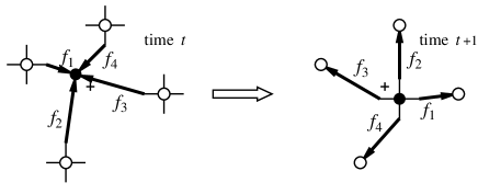
FIG. 1.: Illustration of the way the $\vec{f}_{i}$s are defined. The cross indicates the location of the geometrical center of mass of the four white particles. At the next iteration, the black particle jumps to a symmetrical position with respect to this point.

The motion of all black particles is obtained by updating the above $\vec{f}_{i}$s by equ. (9), with $n=1$ and for $i>0$. The local value of $\vec{\Psi}$ (which is conserved by the dynamics) is then interpreted as the momentum $\vec{p}$ of the corresponding particle. The new location $\vec{r}_{ij}(t+1)$ of particle $ij$ is thus obtained as $\vec{r}_{ij}(t+1)=\vec{r}_{ij}(t)-(1/m_{ij})\vec{\Psi}$, where $m_{ij}$ is a mass associated with the particle. Next, the quantities $\vec{f}$ are propagated to the neighbors and interpreted as the deformations seen by the white particles, which then move according to the same procedure.

A geometrical interpretation of this dynamics is given in fig. 1: for $n=1$, a bulk particle moves to a symmetric location with respect to the center of mass of its neighbors, $(1/4)[\vec{r}_{i-1,j}+\vec{h}+\vec{r}_{i+1,j}-\vec{h}+\vec{r}_{i,j-1}+\vec{u}+\vec{r}_{i,j+1}-\vec{u}]$. Thus, our model corresponds to looking at particles in a harmonic potential, at the particular time where they have maximal displacement and no velocity. Note also that, in this interpretation $\vec{J}_{x}$ and $\vec{J}_{y}$ give, respectively, the separation between the left-right and up-down neighbors.

At the boundary of the domain, or for particles with broken bonds, a different rule of motion has to be considered. The above interpretation, in terms of a jump with respect to the center of mass of the neighbors, gives a natural way to formulate the dynamics when less than four links are present.

Our original wave paradigm includes five fields. In the case of a solid body, the fifth quantity $f_{0}$ can be added in the model as an internal degree of freedom. This is useful in order to describe solids with different sound speeds $c$ and to then see how the fracture propagation speed relates to $c$. The particle motion is still determined by the local momentum $\vec{\Psi}$ but, now, there is no more distinction between white and black particles.

Our goal is now to show that our LB wave model can be used to describe a fracture process. Fracture is a phenomena for which no definite theory is available [13] and a simple model is certainly useful to help understanding generic properties.

At the level of our description, a fracture is easily introduced. A link may break locally if its deformation is too large. Here we consider the energy stored in a link as the quantity determining the breaking. The energy $E_{k}(\vec{r},t)$ of each link $k$, ($k=1$ to $4$) at site $\vec{r}$ and time $t$ is defined as $E_{k}=(1/4)\vec{f}_{0}^{2}+\vec{f}_{k}^{2}$. Since, as mentioned above, our dynamics is unitary, the total energy $E_{{\rm tot}}=\sum_{k,\vec{r}}E_{k}(\vec{r})$ is conserved until a link breaks. Note that, according to our interpretation, the microscopic energy is only of potential type at integer time steps.

The breaking rule we impose is as follows: a link $k$ breaks if the corresponding $E_{k}$ is larger than a given threshold $\epsilon(\vec{r})$ which may, in principle, depend on the position (local defects). Particles with one or more broken links then behave like particles at the boundary.

The total energy $E_{{\rm tot}}$ can be written as the kinetic energy of the center of mass $E_{{\rm kin}}$, plus an internal energy $E_{{\rm int}}\equiv E_{{\rm tot}}-E_{{\rm kin}}$. The kinetic part is computed as $E_{{\rm kin}}=(1/2M)[\sum\vec{p}_{ij}]^{2}$, where $M$ is the total mass.

The second contribution, $E_{{\rm int}}$, can be set proportional to a temperature $T$, using the equipartition theorem. In the initial configuration, $T$ is typically introduced by adding a noise of standard deviation $\sqrt{T}$ to the rest position of each atom.

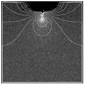
FIG. 2.: Contour plot of the energy $E$ in a $100\times 100$ square solid under a preloaded (mode I) stress ($S=2.2\times 10^{-2}$). The contour line mark the levels $\epsilon/E=10\times\ell$, with $\ell=1,...,10$.

A typical experiment which is performed when studying fracture formation is to apply a stress by pulling in opposite directions the left and right extremities of a solid sample. To achieve a static stress, the solid is prepared in a configuration where the $x$-spacing between the atoms is increased to the value $(1+S)r_{0}$ where $S$ is called the stress factor. Both left and right extremities are not allowed to move. The initial temperature may be different from 0 and a small notch (artificially broken links) is made in the middle of the sample to favor the apparition of the fracture at this position. In the fracture community, this is known as mode I loading [14].

Figure 2 shows the stationary spatial distribution of stress around the notch given by the energy contour lines and obtained from our simulation in a case where the fracture does not propagate across the sample but stops after a few steps. In figure 3 we can see the result of two fracture experiments where the crack spontaneously propagates through the sample after being initiated artificially. The dissipation coefficient $\mu$ in (9) turns out to be essential and eventually distinguishes the two cases presented here. Attenuation prevents the reflection of too much energy from the boundaries toward the crack. With $\mu=0.91$ the dissipation of energy is high enough to limit the acceleration of the crack below some critical speed and the crack remains smooth. On the other hand, with $\mu=0.96$ the crack accelerates above this critical speed and instabilities appear: the crack progresses while making micro-branching.

FIG. 3.: Fracture tip location as a function of time (iterations) for two types of cracks; for comparison, straight lines corresponding to half the speed of sound are drawn. The fastest crack corresponds to a branching situation (see figure 4), obtained for $S=0.03$, $\mu=0.96$, $\epsilon=0.0058$. The slowest crack is smooth (see figure 4) and is produced with $S=0.03$, $\mu=0.91$, $\epsilon=0.0058$.

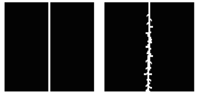
FIG. 4.: Map of the broken links for the smooth (left) and branching cracks (right) described in figure 3.

As can be seen in figure 3, the limiting speed is around half of the speed of sound in the sample. The simulations were performed on samples with $c=1/\sqrt{2}$, but we observe a similar behavior using another values of $c$. Thus, a critical fracture speed [13] of about $c/2$ for the smooth–branching transition is well captured in our model. This non-trivial result is promising since no simple statistical models are yet available to describe a fracture process. The fact that our dynamics is based on a description at the particle level makes the connection with real experiment possible and leaves much flexibility to adjust locally some parameters. Yet, our model is significantly simpler than a molecular dynamics approach. As quantitative experimental results are now possible at a microscopic scale (e.g. scaling in the apparition of micro-cracks before the main crack [15]), our model could contribute to highlight the essential mechanisms of fracture. Another interesting check would be to measure, both numerically and experimentaly the relation between roughness and fracture speed.

We acknowledge support from the Swiss National Science Foundation.

REFERENCES

- [1] Y.H. Qian, S. Succi, and S.A. Orszag. In D. Stauffer, editor, Annual Reviews of Computational Physics III, pages 195–242. World Scientific, 1996.
- [2] B. Chopard and M. Droz. Cellular Automata Modeling of Physical Systems. Cambridge University Press, 1998.
- [3] Y.H. Qian, D. d’Humières, and P. Lallemand. Europhys. Lett, 17(6):470–84, 1992.
- [4] J.D. Jackson. Classical Electrodynamics. John Wiley, 1975.
- [5] P.O. Luthi. PhD thesis, Computer Science Department, University of Geneva, 24 rue General-Dufour, 1211 Geneva 4, Switzerland, 1998.
- [6] B. Chopard, P.O. Luthi, and Jean-Fr d ric Wagen. IEE Proceedings - Microwaves, Antennas and Propagation, 144:251–255, 1997.
- [7] W. J. R. Hoeffer. IEEE Trans. on Microwave Theory and Techniques, MTT-33(10):882–893, October 1985.
- [8] H. J. Hrgovcić. J. Phys. A, 25:1329–1350, 1991.
- [9] C. Vanneste, P. Sebbah, and D. Sornette. Europhys. Lett., 17:715, 1992.
- [10] S. de Toro Arias and C. Vanneste. J. Phys. I France, 7:1071–1096, 1997.
- [11] P. Mora. J. Stat. Phys., 68:591–609, 1992.
- [12] B. Chopard. J. Phys. A, 23:1671–1687, 1990.
- [13] M. Marder and J. Fineberg. Physics Today, pages 24–29, September 1996.
- [14] H.J. Herrmann and S. Roux, editors. Statistical Models for the Fracture of Disordered Media. North-Holland, 1990.
- [15] A. Garcimartin, A. Guarino, and L. Bellon anad S. Ciliberto. Statistical properties of fracture precursors. preprint, 1997.