Influence of wetting properties on hydrodynamic boundary conditions at a fluid-solid interface

Abstract

It is well known that, at a macroscopic level, the boundary condition for a viscous fluid at a solid wall is one of ”no-slip”. The liquid velocity field vanishes at a fixed solid boundary. In this paper, we consider the special case of a liquid that partially wets the solid, i.e. a drop of liquid in equilibrium with its vapor on the solid substrate has a finite contact angle. Using extensive Non-Equilibrium Molecular Dynamics (NEMD) simulations, we show that when the contact angle is large enough, the boundary condition can drastically differ (at a microscopic level) from a ”no-slip” condition. Slipping lengths exceeding 30 molecular diameters are obtained for a contact angle of 140 degrees, characteristic of Mercury on glass. On the basis of a Kubo expression for $\delta$, we derive an expression for the slipping length in terms of equilibrium quantities of the system. The predicted behaviour is in very good agreement with the numerical results for the slipping length obtained in the NEMD simulations. The existence of large slipping lentgh may have important implications for the transport properties in nanoporous media under such ”nonwetting” conditions.

I Introduction

Properties of confined liquids have been the object of constant interest during the last two decades, thanks to the considerable development of Surface Force Apparatus (SFA) techniques. While static properties are now rather well understood (see e.g. [1]), the dynamics of confined systems have been investigated more recently [2]. These studies have motivated much numerical and theoretical work [5, 6, 7, 8, 9, 10] and some progress has been made in giving a simple coherent description of the collective dynamics of confined liquids. Both from experimental and theoretical studies has emerged a rather simple description of the dynamics of not too thin liquid films -i.e. films thicker than typically 10 to 20 atomic sizes. The hydrodynamics of the film can be described by the macroscopic hydrodynamic equations with bulk transport coefficients, supplemented by a ”no-slip” boundary condition applied in the vicinity (i.e. within one molecular layer) of the solid wall. Hence, in spite of the fact that the wall induces a structuration of the fluid into layers that can extend 5 to 6 molecular diameters from the wall, the hydrodynamic properties of the interface are quite simple.

It turns out, however, that all experimental and numerical studies of confined fluids that have been carried out with fluid/substrate combinations that correspond to a total wetting situation. By this we mean that $\gamma_{LS}+\gamma_{LV}<\gamma_{SV}$, where $\gamma$ is a surface energy and the indexes $L$,$V$ and $S$ refere to the liquid, its vapor and the substrate, respectively [17]. In this letter, we investigate the structure and the hydrodynamic properties of a fluid film that is forced to penetrate a narrow pore in a situation of partial wetting, i.e. when $\gamma_{LS}+\gamma_{LV}>\gamma_{SV}$. This corresponds to the case where a drop of the liquid resting on the same substrate, at equilibrium with its vapor, has a finite contact angle which can be deduced from Young’s law $\gamma_{LV}\cos\theta=(\gamma_{SV}-\gamma_{LS})$ [14].

II Model and Results

We first describe our model for the fluid and the substrate, and some details of the simulation procedure. All interactions are of the Lennard-Jones type,

$$v_{ij}(r)=4\epsilon\left(\left({\sigma\over r}\right)^{12}-c_{ij}\left({\sigma\over r}\right)^{6}\right)$$ (1)

with identical interaction energies and molecular diameters $\sigma$. The surface energies will be adjusted by tuning the coefficients $c_{ij}$. In all the simulations that are presented in this letter, the solid substrate is described by atoms fixed on a FCC lattice, with a reduced density $\rho_{S}\sigma^{3}=0.9$. As the atoms are fixed, the coefficient $c_{SS}$ is in fact irrelevant. The interactions between fluid atoms are characterized by $c_{FF}=1.2$, meaning that the fluid under study is more cohesive than the usual Lennard-Jones fluid. The fluid-substrate interaction coefficient $c_{FS}$ will be varied between $0.5$ and $1$. All the simulations will be carried out at a constant reduced temperature, $k_{B}T/\epsilon=1$.

Finally, we mention that the configuration under study will be that of an fluid slab confined between two parallel solid walls. Typically, a configuration contains $10000$ atoms, with a distance between solid walls $h=18\sigma$ and lateral cell dimensions $L_{x}=L_{y}=20\sigma$. Periodic boundary conditions are applied in the $x$ and $y$ directions, i.e. parallel to the walls. For each wall, three layers of FCC solid (in the 100 orientation) will be modelled using point atoms, a continuous attraction between the fluid and the wall in the direction perpendicular to the walls being added in order to model the influence of the deeper solid layers.

All simulations were carried out at constant temperature ($k_{B}T/\epsilon=1$) by coupling the fluid atoms to a Hoover’s thermostat [15]. In flow experiments, only the velocity component in the direction orthogonal to the flow was thermostatted.

Before we discuss in detail the structure of a film, we can roughly estimate the influence of the interaction parameters on the wetting properties of the fluid. Following the standard Laplace estimate of surface energies [14], we have $\gamma_{ij}=-\rho_{i}\rho_{j}\int_{r_{0}}^{\infty}ru_{ij}(r)dr$. Using Young’s law, we obtain for the contact angle $\cos\theta=-1+2\rho_{S}c_{FS}/\rho_{F}c_{FF}$.

From this expression a variation of $c_{FS}$ between 0.5 and 0.9 would be expected to induce a variation of $\theta$ between 100 degrees and 50 degrees. A more accurate determination of the surface tensions was carried out using the method of Nijmeijer et al. [16] The surface tensions are defined in terms of an integral over components of the pressure tensors which can be computed in a simulation. We refer to ref. [16] for more details. The results are listed in table I. By tuning the solid-fluid interaction strength $c_{FS}$ from $c_{FS}=1.0$ to $c_{FS}=0.5$, we found the contact angle deduced from Young’s law varies from $\theta\simeq 90$ degrees to $\theta\simeq 140$ degrees. In figure 1, a typical configuration of a liquid droplet (in coexistence with its vapor) on the solid substrate is shown for $c_{FS}=0.5$, corresponding to $\theta\simeq 140$ degrees. In the following we shall describe such large contact angles (i.e. larger than 90 degrees) as corresponding to a ”nonwetting” situation.

In order to force the fluid into a narrow liquid pore under such partial wetting conditions, an external pressure has to be applied. A simple thermodynamic argument shows that for a parallel slit of width $h$, the minimal pressure is $P_{0}=2(\gamma_{LS}-\gamma_{SV})/h$. For the fluid with $c_{FS}=0.5$, we find, for $h=18\sigma$, $P_{0}=0.079\epsilon/\sigma^{3}$, while $P_{0}=0.018\epsilon/\sigma^{3}$ when $c_{FS}=0.9$. If we use $\sigma=5$Å, $\epsilon=0.05$eV, then $P_{0}\sim$MPa for $h=9$nm in the ”nonwetting” case, $\theta=140$ degrees.

Figure 2 shows the density profiles of the nonwetting fluid inside the pore for pressures corresponding to $2.8P_{0}$ and $16.4P_{0}$. The pressure is changed at constant pore width by changing the number of particles. It is seen in this figures that the highest pressure structure strongly resembles what would be obtained for the usual case of a wetting fluid, with a strong layering at the wall. The structure at the lower pressure is markedly different, with both a layering parallel to the wall and a density depletion near the wall.

We now turn to the study of the dynamical properties of the confined fluid layer. Two types of numerical experiments, corresponding to Couette and Poiseuille planar flows were carried out. In the Couette flow experiments, the upper wall is moved with a velocity $U$ (typically $U=0.5$ in reduced Lennard-Jones units). In the Poiseuille flow experiment, an external force in the $x$ direction is applied to the fluid particles. In figures 3 and 4 we compare the resulting velocity profiles to those that would be expected for a ”no slip” boundary condition applied at one molecular layer from the solid wall. Obviously the velocity profiles for the nonwetting fluid imply a large amount of slip at the solid boundary. As usual, this slippage effect can be quantified by introducing a ”partial slip” boundary condition for the tangential velocity $v_{t}$ at the solid liquid boundary:

$${\partial v_{t}\over\partial z}|_{z=z_{w}}=-{1\over\delta}v_{t}|_{z=z_{w}}.$$ (2)

This boundary condition depends on two parameters, the wall location $z_{w}$ and the slipping length $\delta$. By studying simultaneously Couette and Poiseuille flow for the same fluid film, both parameters can be determined if they are used as fit parameters for the velocity profiles obtained in the simulation. The results of such an adjustment are shown in figures 3 and 4. It turns out that, as was the case in earlier studies [8], the hydrodynamic position $z_{w}$ of the walls is located inside the fluid, typically one atomic distance from the outer layer of solid atoms. Much more interesting is the variation of the slipping length $\delta$, which in earlier work was always found to be very small. In figure 5, the variation of $\delta$ as a function of the pressure is shown for several values of the interaction parameters. The pressure are normalized by the capillary pressure $P_{0}$ defined above as the minimal pressure that must be applied to the fluid in order to enter the pore. For an interaction parameter $c_{FS}=0.9$, corresponding to a contact angle $\theta=100$degrees , the usual behaviour (i.e. a small $\delta$) is obtained. For an interaction parameter $c_{FS}=0.5$ which corresponds to a contact angle $\theta=150$ degrees [18], slipping lengths larger than $15$ molecular diameters can be obtained at the lowest pressures; even at relatively high pressures ($10P_{0}$), the slipping length remains appreciably larger than the molecular size $\sigma$.

III Theory

In order to understand the relation between the hydrodynamic boundary condition and the wetting properties of the fluid on the substrate, one needs to estimate the dependence of the slipping length $\delta$ on the microscopic parameters of the system, such as “roughness”, temperature, $c_{FS}$, etc…

From the “kinetic” point of view, this is obviously a hard task to complete since the slipping length accounts for the ‘parallel’ transfer of momentum between the fluid and the substrate. Explicit calculations can only be done in some model systems [19]. Now in the general case of a dense fluid, no explicit formula for $\delta$ in terms of microscopic quantities is available in the litterature.

In the following, we derive an approximate expression for the slipping length, which will allow us to discuss qualitatively the relationship between wetting and boundary conditions.

Our starting point is a Green-Kubo expression for the slipping length [8] :

$$\lambda={\eta\over\delta}={1\over{Ak_{B}T}}\int_{0}^{+\infty}\langle F_{x}(t).F_{x}(0)\rangle~{}dt$$ (3)

where $\eta$ is the shear viscosity of the fluid, $A=L_{x}L_{y}$ is the lateral solid surface, and $F_{x}$ is the x-component of the total force due to the wall acting on the fluid, at equilibrium (x is a component parallel to the wall). The quantity $\lambda=\eta/\delta$ can be interpreted as the friction coefficient of the fluid/wall interface, relating the force along x due to the wall, to the fluid velocity slip at the wall

$$\langle F_{x}\rangle=-A~{}\lambda~{}V_{slip}$$ (4)

By introducing the density-density correlation function, eq. (3) can be rewritten

$${\eta\over\delta}={1\over{Ak_{B}T}}\int_{0}^{+\infty}dt\int d{\bf r}_{1}\int d{\bf r}_{2}~{}F_{x}({\bf r}_{1})~{}F_{x}({\bf r}_{2})~{}\langle\rho({\bf r}_{1};t)~{}\rho({\bf r}_{2};0))\rangle$$ (5)

The force field $F_{x}({\bf r}_{1})$ derives from the fluid-substrate potential energy $V(xyz)$. The latter has been computed by Steele for a periodic substrate interacting with the fluid through Lennard-Jones interactions [20]. In the case of a (100) face, the main contribution can be written in terms of the shortest reciprocal lattice vectors according to

$$V(xyz)=V_{0}(z)+V_{1}(z)\left\{\cos\left(q_{\parallel}x\right)+\cos\left(q_{\parallel}y\right)\right\}$$ (6)

where $q_{\parallel}=2\pi/a_{s}$ and $a_{s}$ is the lattice spacing in the fcc solid. The altitude $z$ is the distance to the first layer of the atoms of the solid. The functions $V_{0}(z)$ and $V_{1}(z)$ are given by Steele in ref ([20]). In our case however, the attractive parts of $V_{0}(z)$ and $V_{1}(z)$ are multiplied by the tuning factor $c_{FS}$. The force along $x$ is the derivative with respect to $x$ of the interaction potential $V(xyz)$ :

$$F_{x}(x,y,z)=q_{\parallel}~{}V_{1}(z)~{}\sin\left(q_{\parallel}x\right)$$ (7)

When inserted into eq. (5), one obtains

$${\eta\over\delta}={1\over{Ak_{B}T}}\int_{0}^{+\infty}dt\int dx_{1}dy_{1}dz_{1}\int dx_{2}dy_{2}dz_{2}~{}q_{\parallel}^{2}V_{1}(z_{1})V_{1}(z_{2})\sin\left(q_{\parallel}x_{1}\right)\sin\left(q_{\parallel}x_{2}\right)\langle\rho({\bf r}_{1};t)~{}\rho({\bf r}_{2};0))\rangle$$ (8)

We now introduce the Fourier transform of the density in the plane parallel to the substrate

$$\rho_{\bf k}(z)(t)=\int d{\bf x}~{}\rho({\bf x},z;t)~{}e^{i~{}{\bf k}\cdot{\bf x}}$$ (9)

with ${\bf x}=(x,y)$ and the vector ${\bf k}$ is parallel to the substrate. This allows to rewrite the previous equation (8) as

$${\eta\over\delta}={q_{\parallel}^{2}\over{2Ak_{B}T}}~{}\int dz_{1}\int dz_{2}~{}V_{1}(z_{1})~{}V_{1}(z_{2})~{}\int_{0}^{+\infty}dt~{}\Re\left(\langle\rho_{q_{\parallel}}(z_{1})(t)\rho_{-q_{\parallel}}(z_{2})(0)\rangle\right)$$ (10)

with $q_{\parallel}$ in the $x$ direction and $\Re$ stands for the real part. Note that in deriving eq. (10), the homogeneity of the system in the direction parallel to the substrate was taken into account.

Due to the presence of the confining solid, we now assume that the main contribution of $C(q_{\parallel},z_{1},z_{2};t)$ to the time-integral comes from the dynamics in the plane $(x,y)$ parallel to the substrate. Moreover, these dynamics are probed at the first reciprocal lattice vector $q_{\parallel}$. Since $q_{\parallel}$ is close to the position of the first peak in the structure factor, it is reasonable to assume a diffusive relaxation of $\langle\rho_{q_{\parallel}}(z_{1})(t)\rho_{-q_{\parallel}}(z_{2})(0)\rangle$ [21, 22], yielding

$$\langle\rho_{q_{\parallel}}(z_{1})(t)\rho_{-q_{\parallel}}(z_{2})(0)\rangle=exp(-q_{\parallel}^{2}~{}D_{q_{\parallel}}t)~{}\langle\rho_{q_{\parallel}}(z_{1})\rho_{-q_{\parallel}}(z_{2})\rangle$$ (11)

where $D_{q_{\parallel}}$ is a collective diffusion coefficient and $\langle\rho_{q_{\parallel}}(z_{1})\rho_{-q_{\parallel}}(z_{2})\rangle$ is the static correlation function.

The time integration can now be performed to obtain

$${\eta\over\delta}\simeq{1\over{2D_{q_{\parallel}}Ak_{B}T}}~{}\int dz_{1}\int dz_{2}~{}V_{1}(z_{1})~{}V_{1}(z_{2})~{}\langle\rho_{q_{\parallel}}(z_{1})\rho_{-q_{\parallel}}(z_{2})\rangle$$ (12)

so that the slipping length is expressed in terms of static properties of the inhomogeneous system only. A further simplifications can be done by assuming that, due to the stratification near the substrate, the main contribution in the integrals in eq. (12) arises from the $z_{1}\simeq z_{2}$ terms, so that $\langle\rho_{q_{\parallel}}(z_{1})\rho_{-q_{\parallel}}(z_{2})\rangle\simeq A\langle\rho(z_{1})\rangle~{}\delta(z_{1}-z_{2})~{}S(q_{\parallel}|z_{1})$.

The quantity $S(q_{\parallel}|z_{1})$ is the $z$ dependent structure factor, in the plane $z=z_{1}$ (parallel to the solid), defined as

$$S(q_{\parallel}|z_{1})={1\over{A\langle\rho(z_{1})\rangle}}\langle\sum_{i,j}e^{iq_{\parallel}(x_{i}-x_{j})}~{}\delta(z_{i}-z_{1})\rangle$$ (13)

The factor $A\langle\rho(z_{1})\rangle$ ($A$ being the lateral surface) normalizes the average by the number of fluid particles in the layer at the altitude $z_{1}$. If no locking of the fluid occurs near the substrate, one may approximate $S(q_{\parallel}|z_{1})$ by its value at the first layer, $S(q_{\parallel}|z_{1})\simeq S_{1}(q_{\parallel})$. Equation (12) thus reduces to

$${\eta\over\delta}\simeq{S_{1}(q_{\parallel})\over{2D_{q_{\parallel}}~{}k_{B}T}}~{}\int dz_{1}~{}\rho(z_{1})~{}V_{1}(z_{1})^{2}$$ (14)

In order to have a practical estimate to compare with, this formula can be further approximated. The integral term in eq. (14) may be approximated by assuming that it is dominated by the behaviour around the first layer located at $z_{c}\sim\sigma$, so that

$$\int dz~{}\rho(z)~{}V_{1}(z)^{2}\sim\rho_{c}\int_{\sigma}^{+\infty}dz~{}V_{1}(z)^{2}$$ (15)

with $\rho_{c}$ the density at the first layer, denoted in the latter as the “contact” density. Moreover, one expects the “long range” attractive part of $V_{1}(z)$ to contribute mainly to the integral. Since the latter can be written $c_{FS}~{}V^{att}_{1}(z)$, with $V^{att}_{1}(z)$ independent of $c_{FS}$, one gets

$${\delta\over\sigma}\propto{D^{*}_{q_{\parallel}}\over{S_{1}(q_{\parallel})~{}c_{FS}^{2}~{}\rho_{c}\sigma^{3}}}$$ (16)

where $D^{*}_{q_{\parallel}}=D_{q_{\parallel}}/D_{0}$, and $D_{0}=k_{B}T/3\pi\eta\sigma$ is the Stokes-Einstein estimate for the bulk self diffusion coefficient.

All the quantities involved in eq. (16) can be computed in equilibrium Molecular Dynamics simulations. The density at contact $\rho_{c}$ can be measured from density profiles, such as in fig. 2. On the other hand, $D_{q_{\parallel}}$ and $S_{1}(q_{\parallel})$ can be computed from the correlations of density fluctuations in the first layer. In practice, we introduce the function $S_{1}(q_{\parallel},t)=N_{1}^{-1}\langle\rho_{q_{\parallel}}(t)\rho_{q_{\parallel}}(0)\rangle$, where $N_{1}$ is the average number of particles in the first layer and $\rho_{q_{\parallel}}(t)=\sum_{k=1,N_{1}}\exp iq_{\parallel}x_{k}(t)$ is restricted to atoms in the first liquid layer. The value of $S_{1}(q_{\parallel},t)$ at time $t=0$ yields $S_{1}(q_{\parallel})$, while $D_{q_{\parallel}}$ is obtained in terms of the inverse relaxation time of $S_{1}(q_{\parallel},t)$, according to eq. (11) . Let us note at this point that the assumption of an exponential decay of $S_{1}(q_{\parallel},t)$ is indeed verified in the simulations, which allows us to clearly define $D_{q_{\parallel}}$.

In fig. 5, the ratio $\delta/\delta^{*}$, with $\delta^{*}/\sigma=D^{*}_{q_{\parallel}}/{S_{1}(q_{\parallel})c_{FS}^{2}}$ is plotted as a function of the inverse density at contact, $1/\rho_{c}\sigma^{3}$. In these variables, the theoretical estimate, eq. (16), predicts a linear dependence of $\delta/\delta^{*}$ as a function of $1/\rho_{c}\sigma^{3}$. As shown in fig. 5, a linear behaviour $\delta/\delta^{*}=\alpha(1/\rho_{c}\sigma^{3}-1/\rho_{shift}\sigma^{3})$ is indeed observed, in agreement with the prediction. A least-square fit of the datas in this plot gives $\alpha=3.04$ and $1/\rho_{shift}\sigma^{3}=0.47$. The presence of a shift in the density, $1/\rho_{shift}\sigma^{3}$, can be interpreted to account for the higher-order correction in the density at contact which have been neglected in deriving eq. (16) (in particular in the rough approximation assumed in eq. (15)). In the interesting limit where the contact density $\rho_{c}$ is small and $\delta$ is large, this shift does not contribute anymore.

In fig. 5, the full theoretical result for $\delta$

$${\delta\over\sigma}=\alpha{D^{*}_{q_{\parallel}}\over{S_{1}(q_{\parallel})~{}c_{FS}^{2}~{}\rho_{c}\sigma^{3}}}\left(1-{\rho_{c}\over\rho_{shift}}\right)$$ (17)

is plotted as function of $P/P_{0}$ against the measured (out-of-equilibrium) results for $\delta$. The good agreement obtained in these variables for all different pressures and interaction strength $c_{FS}$ emphasize the robustness of the previous theoretical estimate. Obviously, this expression breaks down for very large contact density $rho_{c}>rho_{shift}=2.1\sigma^{3}$, where $\delta$ is expected to vanish anyway.

This result calls for several comments. First, eq. (17) shows that, at for given fluid-substrate interaction $c_{FS}$, $\delta$ decreases with the density and structuration of the fluid in the first layer. The slipping length is thus expected to be quite small in a dense fluid at high pressures, as usually observed and measured experimentally [8, 12]. More specifically, eq. (17) predicts a strong dependence of $\delta$ on the value of the structure factor in the first layer, taken at the shortest reciprocal lattice vector $q_{\parallel}$. This result is in qualitative agreement with previous simulation results [6]. Now if the fluid-substrate interaction $c_{FS}$ is decreased at a given contact density of the fluid $\rho_{c}$ (eg, by increasing simultaneously the pressure), the previous result predicts a strong increase of the slipping length. This explains why substantial slip may be obtained, even if a strong structuration does exist in the fluid, a fact which is a priori counter-intuitive.

Finally, let us come back to the problem of the influence of the wetting properties on the slipping length $\delta$. As noted above, eq. (17) predicts that $\delta$ is a decreasing function of the interaction strength $c_{FS}$. Now, as emphasized for example by the Laplace estimate of the contact angle, $\cos\theta=-1+2\rho_{S}c_{FS}/\rho_{F}c_{FF}$, the contact angle may be interpreted as a “measure” of the fluid-substrate interaction strength $c_{FS}$. In particular one expects the fluid to approach a non-wetting situation ($\cos\theta\rightarrow-1$), when $c_{FS}$ decreases to zero. The previous equation, eq. (17), thus predicts a strong increase of the slipping length $\delta$ when $\cos\theta\rightarrow-1$. In other words in the idealized situation of a non wetting fluid, $\theta=\pi$, a perfect slip may be expected for the boundary condition of the fluid near the surface. The correct trend is observed in our simulation results. This result is in agreement with several experimental observations [25, 26], reporting very large slipping lengths for nonwetting fluids.

IV Conclusions

Obviously the existence of such a large slippage effect should manifest itself in the dynamical properties of a liquid confined in a nanoporous medium. If one considers a single cylindrical capillary, a straightforward calculation in the Poiseuille geometry shows that the existence of slip on the boundaries increases the flow rate in the tube as compared to the “usual” no-slip case by a factor $1+8\delta/h$ (with $h$ the pore diameter and $\delta$ the slip length). Thus, in a porous medium, the effective permeability $K_{eff}$, which relates according to Darcy’s law the flow rate to the pressure drop [23], is expected to increase by the same factor :

$$K_{eff}=K_{0}~{}\left(1+8{\delta\over h}\right)\$$ (18)

where $K_{0}$ is the ”standard” permeability, obtained within the no slip assumption (i.e., when $\delta$ is zero). In a wetting situation, $\delta$ is obtained to be very small and $K_{eff}\simeq K_{0}$. However, in a nonwetting situation ($\theta\sim 140$ degrees), the slipping length $\delta$ may largely exceed the nanometric pore sizes $h$, so that the effective permeability $K_{eff}$ is expected to be much larger than $K_{0}$ (say, more that one order of magnitude in view of the prefactors).

It can also be expected that the microscopic dynamics of the molecules could be rather different in a ”nonwetting” medium, compared to what it is in the bulk or in a medium with strong solid/liquid affinity. In fact, recent studies point towards the importance of the surface treatment for the reorientation dynamics of small molecules in nanopores [24]. Correlating the wetting properties with such microscopic studies seems to be a promising area for future research.

This work was supported by the Pole Scientifique de Modélisation Numérique at ENS-Lyon, the CDCSP at the University of Lyon, the DGA and the French Ministry of Education under contract 98/1776. We would like to thank E. Charlaix and P.-F. Gobin for introducing us to this subject, and Dr. S.J. Plimpton for making publicly available a parallel MD code [27], a modified version of which was used in the present simulations. References [25, 26] were pointed out to us by Dr. Remmelt Pit.

TABLE I.: Dependence of the surface tensions (in units of $\epsilon$) and contact angle $\theta$ (in degrees), on the tuning parameter $c_{FS}$. The liquid-vapour surface tension was determined independently to be $\gamma_{LV}=0.94~{}\epsilon$.

$c_{FS}$	$\gamma_{SV}-\gamma_{LS}$	$\cos(\theta)$	$\theta$
0.5	-0.71	-0.74	137
0.6	-0.65	-0.68	133
0.7	-0.50	-0.52	121
0.8	-0.35	-0.36	111
0.9	-0.16	-0.17	99

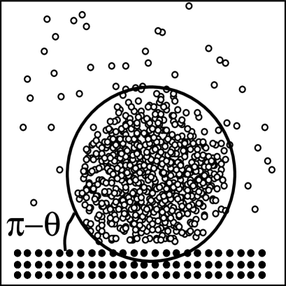
FIG. 1.: A typical configuration of a liquid droplet (1000 atoms) on a solid substrate in a ”nonwetting” case ($c_{FS}=0.5$), in equilibrium with its vapor. This configuration was prepared by starting from an homogeneous fluid slab of thickness $18\sigma$, confined between two walls. The droplet is formed by simultaneously increasing moving the upper wall by $20\sigma$ in the $z$ direction and removing the fluid atoms that lie near the box boundaries. The bounding box has a size of $20\sigma$.

FIG. 2.: Density profiles of the ”nonwetting” fluid ($c_{FS}=0.5$) confined between two solid walls separated by 20$\sigma$. The positions of the first layer of solid atoms have been indicated by vertical dashlines. Full line: $P/P_{0}=2.8$; dashed line: $P/P_{0}=16.4$. The latter curve has been shifted upwards for clarity.

FIG. 3.: Velocity profile (in reduced units) of the ”nonwetting” fluid ($c_{FS}=0.5$) in a Couette geometry. The reduced pressure is $P/P_{0}\simeq 7.3$. The solid line is the simulation result, the dashed line is a linear fit of the numerical results, and the dashed-dot line is the velocity profile predicted by the no-slip bounbary condition. The velocity of the upper wall is $U=0.5$.

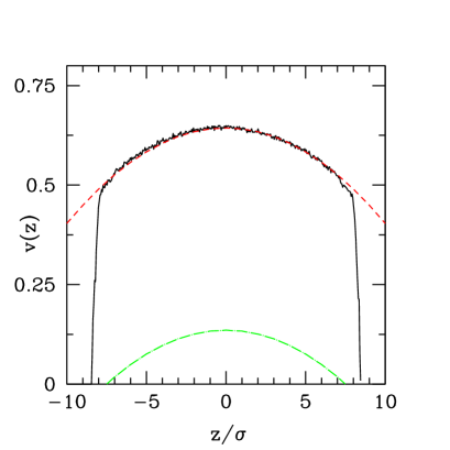
FIG. 4.: Same as in figure 3, but in a Poiseuille geometry. The external force applied on each fluid particle is $f_{ext}=0.02\epsilon/\sigma$

FIG. 5.: Variation of the slipping length $\delta$ (in units of $\sigma$) as a function of the reduced pressure $P/P_{0}$, for several values of the interaction parameters $c_{FS}$. From top to bottom, the datas correspond to $c_{FS}=0.5$, $c_{FS}=0.6$, $c_{FS}=0.7$, $c_{FS}=0.8$, $c_{FS}=0.9$. Solid lines are the theoretical prediction, eq. (17) (see text for details).

FIG. 6.: Normalized slipping length $\delta/\delta^{*}$, with $\delta^{*}=\sigma D^{*}_{q_{\parallel}}/{S_{1}(q_{\parallel})c_{FS}^{2}}$, as a function of the inverse contact density $1/\rho_{c}\sigma^{3}$. In this plot, a linear dependence is expected according to the theoretical prediction, eq. (16). The dashed line is a least-square fit of the numerical datas, with slope $\alpha=3.04$ and shift in inverse density $1/\rho_{shift}\sigma^{3}=0.47$.

REFERENCES

- [1] J.N. Israelachvili, Intermolecular and Surface Forces (Academic Press, London, 1985)
- [2] J.M. Drake, J. Klafter and R. Kopelman (eds), Dynamics in small confining systems (MRS, Pittsburgh, 1996)
- [3] G.K. Batchelor, An Introduction to Fluid Dynamics, (Cambridge University Press, Cambridge, 1967)
- [4] D.Y.C. Chan and R.G. Horn, J. Chem. Phys. 83, 5311 (1985)
- [5] J. Koplik, J.R. Benavar and J.F. Willemsen, Phys. Rev. Lett. 60, 1282 (1988)
- [6] P.A. Thompson and M.O. Robbins, Phys. Rev. A 41, 6830 (1990)
- [7] I. Bitsanis, S.A. Somers, H.T. Davis and M. Tirrell, J. Chem. Phys. 93, 3427 (1990)
- [8] L. Bocquet and J-L. Barrat, Phys. Rev. E 49, 3079 (1994);and J. Phys. : Cond. Matt. 8, 9297 (1996).
- [9] C.J. Mundy, S. Balasubramanian, K. Bagchi, J.I. Siepmann, M.L. Klein, FARADAY DISCUSSIONS, 104, 17 (1996)
- [10] K. Koplik, J.R. Banavar, Phys. Rev. Lett. 23, 5125 (1998).
- [11] H.W. Hu, G.A. Carson and S. Granick, Phys. Rev. Lett. 66,2758 (1991)
- [12] J-M. Georges, S. Millot, J-L. Loubet and A. Tonck, J. Chem. Phys. 98, 7345 (1993)
- [13] J.N. Israelachvili, P.M. McGuiggan and A.M. Homola, Science, 240, 189 (1988)
- [14] J.S. Rowlinson and B. Widom, Molecular Theory of Capillarity (Oxford University Press, Oxford, 1989)
- [15] M. Allen, D. Tildesley, Computer simulation of liquids (Oxford University Press, Oxford, 1987)
- [16] M.J.P. Nijmeijer, C. Bruin, A.F. Bakker, J.M.J van Leeuwen, Phys. Rev. A 42, 6052 (1990).
- [17] We mention that in some numerical simulations, purely repulsive interactions between the fluid and the substrate were considered. In that case, however, the pressure of the fluid is very high, and the properties of the confined fluid is very similar to what is obtained for a wetting fluid (with attractive interactions to the substrate) at a lower pressure.
- [18] The contact angle of mercury on glass is typically 140 degrees.
- [19] L. Bocquet, C. R. Acad. Sci. Paris, 316, Serie II, 7 (1993).
- [20] W.A. Steele, Surf. Sci. 36 317 (1973).
- [21] P.G. de Gennes, Physica 25, 825 (1959)
- [22] J.P. Boon and S. Yip, Molecular Hydrodynamics (Dover Publications, New York, 1980).
- [23] J. Bear Dynamics of fluids in porous media (Elsevier, New-York, 1972)
- [24] M. Arndt, R. Stannarius, W. Gorbatschow, F. Kremer, Phys. Rev. E, Vol.54, 5377 (1996)
- [25] N.V. Churaev, V.D. Sobolev, A.N. Somov, J. Colloid and Interface Science, 147, 574 (1984)
- [26] T.D. Blake, Colloids and Surfaces, 147, 135 (1990) and references therein.
- [27] S.J. Plimpton, J. Comp. Physics. 117, 1 (1995); code available at http://www.cs.sandia.gov/tech_reports/sjplimp