Lectures on Non Perturbative Field Theory
and Quantum Impurity Problems.

These are lectures presented at the Les Houches Summer School “Topology and Geometry in Physics”, July 1998. They provide a simple introduction to non perturbative methods of field theory in $1+1$ dimensions, and their application to the study of strongly correlated condensed matter problems - in particular quantum impurity problems. The level is moderately advanced, and takes the student all the way to the most recent progress in the field: many exercises and additional references are provided.

In the first part, I give a sketchy introduction to conformal field theory. I then explain how boundary conformal invariance can be used to classify and study low energy, strong coupling fixed points in quantum impurity problems. In the second part, I discuss quantum integrability from the point of view of perturbed conformal field theory, with a special emphasis on the recent ideas of massless scattering. I then explain how these ideas allow the computation of (experimentally measurable) transport properties in cross-over regimes. The case of edge states tunneling in the fractional quantum Hall effect is used throughout the lectures as an example of application.

Introduction

Quantum impurity problems have been for many years, and increasingly so recently, a favorite subject of investigations, for theorists and experimentalists alike. There are many good reasons for that.

First, these problems often represent the simplest setting in which some qualitatively fascinating physical properties can be observed and probed. For instance, the Kondo model (for a comprehensive review , consult [1]) provides a clear cut example of asymptotic freedom. The basic experimental fact is that normal metals with dilute impurities exhibit an unusual minimum in the temperature dependence of the electrical resistivity. The ultimate explanation is that the interaction of the electrons with the impurity spins produces an increase of the resistivity as $T$ is lowered, counteracting the usual decrease in resistivity arising from interactions with lattice phonons. Low temperature means low energy, or large distance: we thus have a problem where interactions increase at large distance, a characteristic of asymptotic freedom . As another example I would like to mention the recent experiments [2, 3] about point contact tunneling in the fractional quantum Hall effect (for a review on this active topic, see [4]) at filling fraction $\nu={1\over 3}$. Measurments of the shot noise reveal a behaviour $\left<I^{2}\right>\propto{e\over 3}I_{B}$ in the limit of weak backscattering, where few quasiparticles tunnel, and do so independently. If one compares this formula with the standard Schottky formula for Fermi liquids, one sees that this noise has to be due to the tunneling of fractional charges $e^{*}={e\over 3}$: although the existence of these (Laughlin quasiparticles) had been conjectured for a long time, the noise is the first direct evidence of their existence . As a final example, let me recall that the basic archetype of dissipative quantum mechanics (for a review, look at [5], [6]), the two state problem coupled to a bath of oscillators with Ohmic dissipation, is described by another quantum impurity problem: the anisotropic Kondo model. Crucial fundamental issues are at stake here, as well as a large array of applications in chemistry and biology.

The second reason of our fascination for quantum impurity problems is that they are, to a large extent, manageable by analytic methods. This has led to incredibly fruitful progress in the past. For instance, the renormalization group was, to a large extent, borne out of the efforts of Kondo, Anderson and Wilson to understand the low temperature behaviour of the Kondo model (see [1]). Also, the works of Andrei [7], Wiegmann [8] and others showed that the Bethe ansatz could be used to analyze situations of experimental relevance: this spurred a new interest in quantum integrable models, an area which, together with its various off-springs like quantum groups, knot theory and others, has become one of most lively in mathematical physics.

Finally, it is fair to say that quantum impurity problems are not only of fundamental interest: they are at the center of the most challenging problems of today’s condensed matter, like Kondo lattices, heavy fermions, and, maybe, high $T_{c}$ superconductors.

In these lectures, I will concentrate on what is usually considered the most important about quantum impurity problems: their properties as strongly interacting systems. There is no doubt that strongly correlated electrons are of the highest interest. On the practical side, besides high $T_{c}$ superconductivity, let me mention the remarkable recent developments in manufacturing and understanding small systems like quantum wires, carbon nanotubes and the like, where, because of the reduced dimensionality, Fermi liquid theory is not applicable, and the interactions have to be taken into account non perturbatively. On a more fundamental level, strongly interacting systems exhibit rather counter intuitive properties, the most spectacular being probably spin charge separation. It is a challenge for the theorist to understand these properties, and quantum impurity problems no doubt provide the best theoretical and experimental laboratory to do so.

Maybe it is time now to define what I mean by a quantum impurity problem. The general class of systems I have in mind have the following features: $(i)$ There are extended gapless (critical) quantum mechanical degrees of freedom, which live in an infinite spatial volume, the “bulk” $(ii)$ These interact with an impurity, localized at one point in position space. This impurity may carry quantum mechanical degrees of freedom.

To have an example in mind, consider the Kondo problem: (i) The extended degrees of freedom are those of the bulk metal. The presence of a Fermi surface means that the metal sits at a RG fixed point (see e.g. [9]). Physically this is easily understood since the system of electrons has (“particle-hole”) excitations of arbitrarily low energy about its Fermi-sea ground state, providing the critical degrees of freedom in the bulk of the metal (ii) The impurity spin, located at one point in space (say the origin), is a dynamical quantum mechanical degree of freedom (the dynamical process is the spin-flip).

In the Kondo model we also see another feature of quantum impurity problems: they are generically one-dimensional. The problem of an impurity in a Luttinger liquid to be discussed below is inherently one-dimensional, but the Kondo model needs to be reduced to one dimension. Since the impurity spin sits only at one point in space, it is only the s-wave wavefunctions of the metal electrons that can interact with the spin. Second-quantizing this s-wave theory, we get a (non-interacting) quantum field theory of one-dimensional Fermions, defined on half-infinite (radial) position space (a half-infinite line), which interacts with the quantum spin at the end of the line. Considering a path-integral representation of the 1D theory of Fermions, we have a $(1+1)$-dimensional Lagrangian field theory, one dimension from the (half-infinite) radial space coordinate, and another dimension from the (say, euclidean) time coordinate. All interactions take place at one point in space, the end of the line, where the impurity is located. In the $(1+1)$ dimensional space-time picture, the impurity sits at the “boundary” of space-time, which can be viewed as the upper-complex plane, the “boundary” being the real axis (these points of view are schematically illustrated in figure 1 and 2). This will be the general picture that we use in the study of all quantum impurity problems.

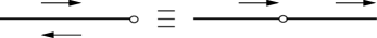
Figure 1: We will think of quantum impurity problems in various ways. The figure on the left represents a $1+1$ quantum point of view where the bulk right and left degrees of freedom are confined to a half line, with the impurity at the origin. Altrnatively, because the theory is massless in the bulk, one can unfold this picture to get only right degrees of freedom on the full line, as indicated on the right.

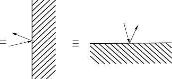
Figure 2: Alternatively again, one can go to imaginary time and obtain a $2$D statistical mechanics point of view, with a theory defined in a half plane, that often we will chose to be the upper complex plane. In this figure, the arrows are supposed to “represent” the bulk degrees of freedom; later, we will see that they can be associated with integrable quasiparticles.

In the Kondo problem we see one way how a quantum impurity problem can be realized experimentally: a bulk system (here the 3D metal) contains a finite but small concentration $x$ of quantum impurities. In the limit of very dilute impurities ($x<1$) the impurities do not interact with each other (to lowest order in $x$), and the single-impurity theory may be used to describe the physics of the bulk material in the presence of dilute impurities. Actually, experiments performed at very low concentrations are known to be in good agreement with the single-impurity theory for the ordinary (one-channel) Kondo model.

A quite different realization of quantum impurity models occurs in the context of point contacts. These are basically electronic devices: two leads (capable of transporting electrical current) are attached to a single quantum impurity. Each one of the leads is connected to a battery, so that electrical current is driven through the quantum impurity. One can then measure experimentally the electrical current $I$, flowing through the quantum impurity, as a function of the applied driving voltage $V$ (from the battery) [10]. The $I(V)$ curve, the differential (non-linear) conductance $G_{diff}=\partial I(V)/\partial V$, or the temperature dependence of the linear response conductance $G_{lr}=\lim_{V\to 0}I(V)/V$ are examples of experimental probes characteristic of the quantum impurity. Notice that since the $I(V)$ curve as well as the differential conductance are non-equilibrium properties, the point-contact realizations of quantum impurity problems are theoretically more challenging than other realizations, in that more than equilibrium statistical mechanics is involved to achieve a theoretical understanding of these quantities.

Ideally, the most interesting point contact situation would involve one-dimensional leads, where electrons are described by the Luttinger model, the simplest non-fermi-liquid metals [11]. It consists of left- and right-moving gapless excitations at the two fermi points in an interacting 1-dimensional electron gas. In the past, this model had been difficult to realize experimentally however. This is simply because in a one-dimensional conductor (such as a quasi-one-dimensional quantum wire so thin that the transverse modes are frozen out at low temperature), random impurities occur in the fabrication. These impurities lead to localization due to backscattering processes between the excitations at the two fermi points. In other words, the random impurities generate a mass gap for the fermions.

Fortunately, there is another possiblity: the edge excitations at the boundary of samples prepared in a fractional quantum Hall state should be extremely clean realizations of the Luttinger non-fermi liquids, as was observed by Wen [12]. In contrast to quantum wires, these are stable systems because for $1/\nu$ an odd integer, the excitations only move in one direction on a given edge. Since the right and left edges are far apart from each other, backscattering processes due to random impurities in the bulk cannot localize those extended edge states. Moreover, the Luttinger interaction parameter is universally related to the filling fraction $\nu$ of the quantum Hall state in the bulk sample by a topological argument based on the underlying Chern-Simons theory, and does therefore not renormalize. The edge states should thus provide an extremely clean experimental realization of the Luttinger model.

We now describe an experimental set-up in more details [13, 14] (see figure 3).

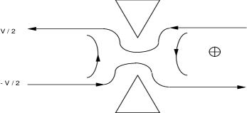
Figure 3: A schematic experimental set up to study point contact tunneling in the fractional quantum Hall effect (the magnetic field points towards the reader). Details are provided in the text.

A fractional quantum Hall state with filling fraction $\nu=1/3$ is prepared in the bulk of a quantum Hall bar which is long in the $x$-direction and short in the $y$-direction. This means that the bulk quantum Hall state is prepared in a Hall insulator state (longitudinal conductivity $\sigma_{xx}=0$), and that the (bulk) Hall resistivity is on the $\nu=1/3$ plateau where $\sigma_{xy}=(1/3)e^{2}/h$. This is achieved by adjusting the applied magnetic field, perpendicular to the plane of the bar. Since the plateau is broad, the applied magnetic field can be varied over a significant range without affecting the filling of $\nu=1/3$. Next, a gate voltage $V_{g}$ is applied perpendicular to the long side of the bar, i.e. in the $y$ direction at $x=0$. This has the effect of bringing the right and left moving edges close to each other near $x=0$, forming a point contact. Away from the contact there is no backscattering (i.e. no tunneling of charge carriers) because the edges are widely separated, but now charge carriers can hop from one edge to the other at the point contact.

The left-moving (upper) edge of the Hall bar can now be connected to battery on the right such that the charge carriers are injected into the left-moving lead of the Hall bar with an equilibrium thermal distribution at chemical potential $\mu_{L}$. Similarly, the right-moving carriers (propagating in the lower edge) are injected from the left, with a thermal distribution at chemical potential $\mu_{R}$. The difference of chemical potentials of the injected charge carriers is the driving voltage $V=\mu_{R}-\mu_{L}$. If $V>0$, there are more carriers injected from the left than from the right, and a “source-drain” current flows from the left to the right, along the $x$-direction of the Hall bar. In the absence of the point contact, the driving voltage places the right and left edges at different potentials (in the $y$-direction, perpendicular to the current flow), implying that the ratio of source-drain current to the driving voltage $V$ is the Hall conductance $G=\nu e^{2}/h$ (both in linear response and at finite driving voltage $V$). When the point-contact interaction is included, at finite driving voltage, more of the right moving carriers injected from the left are backscattered than those injected from the right, resulting in a loss of charge carriers from the source-drain current. In this case we write the total source-drain current as $I(V)=I_{0}(V)+I_{B}(V)$, where $I_{B}(V)$ is the (negative) backscattering current, quantifying the loss of current due to backscattering at the point contact. It is this backscattering current that I ultimately want to show how to compute.

Let me write up some formulas as a preamble. I will not have time in these lectures to discuss bosonization or edge states in the fractional quantum Hall effect: I will thus simply claim that, in its bosonized form, the problem is described by the hamiltonian

$$H={1\over 2}\int_{-\infty}^{\infty}dx\left[\Pi^{2}+(\partial_{x}\phi)^{2}\right]+\lambda\cos{\beta\over\sqrt{2}}(\phi_{L}-\phi_{R})(0),$$ (1)

where ${\beta^{2}\over 8\pi}=\nu$. Here, the free boson part describes the massless edge states [12], and the cosine term describes the effect of the gate voltage, with $\lambda\propto V_{g}$. In general of course, the backscattering term induced by this gate voltage should be represented by a complicated interaction; but we keep only the most relevant term (the only one for $\nu={1\over 3}$), which is all that matters in the scaling regime (see below) we will be interested in.

The interaction is a relevant term, that is, in a renormalization group transformation, one has, $b$ being the rescaling factor

$${d\lambda\over db}=(1-\nu)\lambda+O(\lambda^{3})$$ (2)

This means that at large gate voltage, or, equivalently, at small temperature (since then, elementary excitations have low energies, so the barrier appears big to them), the point contact will essentially split the system in half, and no current will flow through . The questions the theorist wants to answer are: how do we study the vicinity of the weak-backscattering limit? How do we find out more precisely what the strong back-scattering limit looks like? How about its vicinity? Finally, can we be more ambitious and compute say the current at any temperature, voltage and gate voltage?

For this latter question, let me stress that we are interested in the universal, or scaling, regime, which is the only case where things will not depend in an complicated way on the microscopic details of the gate and other experimental parameters. In practice, what the experimentalist will do is first sweep through values of the gate voltage, the conductance signal showing a number of resonance peaks, which sharpen as the temperature is lowered. These resonance peaks occur for particular values $V_{g}=V_{g}^{*}$ of the gate voltage, due to tunneling through localized states in the vicinity of the point contact. Ideally, on resonance, the source-drain conductance is equal to the Hall conductance without point contact, i.e. $G_{resonance}=\nu e^{2}/h$. This value is independent of temperature, on resonance. Now, measuring for instance the linear response conductance as a function of the gate voltage near the resonance, i.e. as a function of $\delta V_{g}\equiv V_{g}-V_{g}^{*}$, at a number of different temperatures $T$, one gets resonance curves, one for each temperature. These peak at $\delta V_{g}=0$. Finally, these conductance curves should collapse, in the limit of very small $T$ and $\delta V_{g}$, onto a single universal curve when plotted as a function of $\delta V_{g}/T^{1-\nu}$. This is what the field theorist wants to compute.

To proceed, it is useful to formulate the problem as a boundary problem. For this, a few manipulations are needed . We decompose $\phi=\phi_{L}+\phi_{R}$ and set :

$$\varphi^{e}(x+t)={1\over\sqrt{2}}\left[\phi_{L}(x,t)+\phi_{R}(-x,t)\right]$$

$$\varphi^{o}(x+t)={1\over\sqrt{2}}\left[\phi_{L}(x,t)-\phi_{R}(-x,t)\right]$$ (3)

Observe that these two fields are left movers. We now fold the system by setting, for $x<0$ :

$$\phi^{e}_{L}=\varphi^{e}(x+t),~{}~{}~{}~{}~{}~{}~{}\phi^{e}_{R}=\varphi^{e}(-x+t),$$

$$\phi^{o}_{L}=\varphi^{o}(x+t),~{}~{}~{}~{}~{}~{}~{}\phi^{o}_{R}=-\varphi^{o}(-x+t),$$ (4)

and introduce new fields $\phi^{e,o}=\phi^{e,o}_{L}+\phi^{e,o}_{R}$, both defined on the half infinite line $x<0$. The odd field $\phi^{e}$ simply obeys Dirichlet boundary conditions at the origin $\phi^{o}(0)=0$, and decouples from the problem. The field $\phi^{e}$, which we call rather $\Phi$ in the following, has a non trivial dynamics

$$H\equiv H^{e}=\frac{1}{2}\int_{-\infty}^{0}dx\ \left[\Pi^{2}+(\partial_{x}\Phi)^{2}\right]+\lambda\cos\frac{\beta\Phi(0)}{2}.$$ (5)

The aspects we have to understand are, by increasing order of complexity: the fixed points, their vicinity, and what is in between. This is the order I will follow in these lectures.

Part I Conformal field theory and fixed points

The first difficulty one encounters in that field is how to describe the low energy fixed points. This may sound rather simple in the tunneling problem, but in other cases, for instance in a tunneling problem for electrons with spin, the matter is quite involved. The reason for this is, that fixed points are not necessarily described in terms of nice linear boundary conditions for the bulk degrees of freedom. It does seem to be true however, that even if the quantum impurity has internal degrees of freedom, interaction and renormalization effects do turn the dynamical quantum impurity into a boundary condition on the extended bulk degrees of freedom, at large distances, low energy or low temperature. At low temperatures the system may be in the strong coupling regime (for instance, this is where Kondo’s result diverges). The boundary condition is thus a way to think about the strongly interacting system. Nozières’ physical picture of screening [15] illustrates how this works for the simplest case, the one-channel Kondo model: the antiferromagnetic interaction of the impurity spin with the spin of the conduction electrons, which has renormalized to large values at low temperatures, causes complete screening of the impurity spin. A modified boundary condition on the electrons that are not involved in the screening, is left. This mechanism, however, appears to be much more general, and seems to apply to all quantum impurity problems.

The boundary conditions generated in this process may be highly non-trivial (see e.g. [17, 18]). However, since the bulk is massless (critical), the induced boundary condition is scale invariant asymptotically at large distances and low temperatures. Actually, it is, in most cases, conformally invariant.

Quantum impurity problems are thus intimately related with scale-invariant boundary conditions: these are RG fixed points, and, like in bulk $1+1$ quantum field theories, (recall that the bulk is always critical in the type of systems that we are considering here), conformal symmetry is the best way to describe them.

Now, conformal invariance is a long story. All I can do is provide, in the next sections, what I believe is the minimal set of ideas necessary to understand what is going on, and tackle without fear the literature on the subject. In several instances, I will have to discard entire discussions of key issues, substituting them with some intuitive comments, and only providing the final result. Additional bits and pieces are then provided in the text in small characters, together with specific references, to help the reader bridge the gaps. Good reviews on this subject are the Les Houches Lectures of 1988 [19], the article by J. Cardy [20], the lectures by J. Polchinski [21], and the textbook [22]. The relevant chapters in [23] can also be quite useful.

In the following, I will intimately mix path integral and hamiltonian points of view. The two are of course equivalent, but each has its own advantages.

1 Some notions of conformal field theory

1.1 The free boson via path integrals

We consider the free bosonic theory, with action

$$S={1\over 2}\int dx_{1}dx_{2}\left[\left(\partial_{1}\Phi\right)^{2}+\left(\partial_{2}\Phi\right)^{2}\right]$$ (6)

To start, let us discuss briefly the issue of correlators and regularization. To keep in the spirit of condensed matter, we initially define the Gaussian model on a discrete periodic square lattice of constant $a$ by setting

$$S_{latt}={1\over 2}\sum_{\left<jk\right>}\left[\Phi(r_{j})-\Phi(r_{k})\right]^{2},$$ (7)

where the sum is taken over all pairs of nearest neighbours. Introduce the lattice Green function

$$G_{latt}(r)={1\over L^{2}}\sum^{\prime}_{n_{1},n_{2}}{e^{ik.r}\over 4-2\cos{2\pi n_{1}a\over L}-2\cos{2\pi n_{2}a\over L}}$$ (8)

where the sum is restricted to the first Brillouin zone $|n_{i}|\leq{L\over 2a}$, and the prime means the zero mode is excluded . One has then (where the points $r,r^{\prime}$ belong to the lattice)

$$\left<\Phi(r)\Phi(r^{\prime})\right>_{latt}=G_{latt}(r-r^{\prime})$$ (9)

while $G_{latt}$ satisfies the discrete equation (where $\Delta_{latt}$ is the discrete Laplacian)

$$\Delta_{latt}G_{latt}=-\delta_{latt}(r)$$ (10)

The important points here are the behaviours $G_{latt}(0)\approx-{1\over 2\pi}\ln{a\over L},L>>a$, and $G_{latt}(r)\approx-{1\over 2\pi}\ln{r\over L}$ for $a<<r<<L$.

We recall now Wick’s theorem, according to which the average of any quantity can be obtained as a sum of all pairwise contractions. It follows that

$$\left<e^{i\beta_{1}\Phi(r)}e^{i\beta_{2}\Phi(r^{\prime})}\right>_{latt}= \exp\left[-{1\over 2}(\beta_{1}+\beta_{2})^{2}\left<\Phi^{2}(r)\right>_{latt}\right]$$ (11)

$$\times\exp\left[-\beta_{1}\beta_{2}\left(\left<\Phi(r)\Phi(r^{\prime})\right>_{latt}-\left<\Phi^{2}(r)\right>_{latt}\right)\right]$$

To define a continuum limit for this model, we look at distances large compared to the lattice spacing but small compared to $L$, where the right hand side of the previous expression simplifies into

$$\left<e^{i\beta_{1}\Phi(r)}e^{i\beta_{2}\Phi(r^{\prime})}\right>_{latt}\approx\left({a\over L}\right)^{(\beta_{1}+\beta_{2})^{2}/4\pi}\left({|r-r^{\prime}|\over a}\right)^{\beta_{1}\beta_{2}/2\pi}$$ (12)

The well known observation follows that the correlator vanishes unless charge neutrality is satisfied, that is $\beta_{1}+\beta_{2}=0$. We then have, where $r,r^{\prime}$ are now arbitrary points in the continuum,

$$\left<e^{i\beta\Phi(r)}e^{-i\beta\Phi(r^{\prime})}\right>\approx\left({a\over|r-r^{\prime}|}\right)^{\beta^{2}/2\pi}$$ (13)

In the following we will sometimes, but not always, set $a=1$.

1.2 Normal ordering and OPE

We now introduce complex coordinates $z=x_{1}+ix_{2},\bar{z}=x_{1}-ix_{2}$. We have $\partial={1\over 2}(\partial_{1}-i\partial_{2}),\bar{\partial}={1\over 2}(\partial_{1}+i\partial_{2})$, $d^{2}z=2dx_{1}dx_{2}$, and we define the delta function by $\int d^{2}z\delta^{2}(z,\bar{z})=1$, so $\delta^{2}(z,\bar{z})={1\over 2}\delta^{2}(x_{1},x_{2})$. The action reads now

$$S=\int d^{2}z\partial\Phi\bar{\partial}\Phi,$$ (14)

and the laplacian

$$\Delta=2\partial\bar{\partial}+2\bar{\partial}\partial$$ (15)

Of crucial importance is the result

$$\partial\left({1\over\bar{z}}\right)=2\pi\delta^{2}(z,\bar{z})$$ (16)

from which it follows that

$$\partial\bar{\partial}\ln|z|^{2}=\partial\bar{\partial}\ln\bar{z}=2\pi\delta^{2}(z,\bar{z})$$ (17)

It is customary to write the basic correlator as

$$\left<\Phi(z,\bar{z})\Phi(z^{\prime},\bar{z}^{\prime})\right>=-{1\over 4\pi}\ln|z-z^{\prime}|^{2}$$ (18)

Note that, in this expression, we have completely discarded the $L$ dependence that occurs in the lattice system. A reason for doing so is that $\Phi$ is not a “good” field anyway, and that we will usually consider rather derivatives of $\Phi$, for which this ambiguity does not matter. The $L$ dependence is however crucial for exponentials of the field $\Phi$. When we discard it, we have to remember that, at the end of the day, only correlators which have vanishing charge are non zero.

Now, still using Wick’s theorem it follows that

$$\partial\bar{\partial}\left<\Phi(z,\bar{z})\Phi(z^{\prime},\bar{z}^{\prime})\ldots\right>=-{1\over 2}\left<\delta^{2}(z-z^{\prime},\bar{z}-\bar{z}^{\prime})\ldots\right>,$$ (19)

where the dots stand for any other insertions in the path integrals, that involve no field either at $z$ or $z^{\prime}$. A relation that holds in this sense is simply rewritten

$$\partial\bar{\partial}\Phi(z,\bar{z})\Phi(z^{\prime},\bar{z}^{\prime})=-{1\over 2}\delta^{2}(z-z^{\prime},\bar{z}-\bar{z}^{\prime}).$$ (20)

This is the first example of equations we will write quite often between “operators” in the theory - the word operator here occurs naturally when one splits open the path integral to obtain a hamiltonian description, see later.

Recall that the equations of motion for the field $\Phi$ read, on the other hand

$$\partial\bar{\partial}\Phi(z,\bar{z})=0$$ (21)

It follows that the product $\Phi(z,\bar{z})\Phi(z^{\prime},{\bar{z}}^{\prime})$ obeys the equation of motion except at coincident points.

In the sequel, we shall constantly use the concept of normal ordering. We define the normal ordering of the product of two bosonic fields by

$$:\Phi(z,\bar{z})\Phi(z^{\prime},\bar{z}^{\prime}):\equiv\Phi(z,\bar{z})\Phi(z^{\prime},\bar{z}^{\prime})+{1\over 4\pi}\ln|z-z^{\prime}|^{2}$$ (22)

This definition is such that the normal ordered product of fields now does satisfy the equation of motion even at coincident points

$$\partial\bar{\partial}:\Phi(z,\bar{z})\Phi(z^{\prime},\bar{z}^{\prime}):=0$$ (23)

As a result of this, the normal product is (locally) the sum of an analytic and antianalytic function, and can be expanded in powers of $z$. Thus, for instance

$$\Phi(z,\bar{z})\Phi(0,0)=-{1\over 4\pi}\ln|z|^{2}+:\Phi^{2}(0,0):+z:\partial\Phi\Phi(0,0):+\bar{z}:\bar{\partial}\Phi\Phi(0,0):+\ldots$$ (24)

This is the first example of an operator product expansion (OPE). Like equation (20), its precise meaning is that it holds once inserted inside a correlation function. OPEs in conformal field theories are not asymptotic, but rather convergent expansions; their radius of convergence is given by the distance to the nearest other operator in the correlation functions of interest. The right hand side of (24) involves products of fields at coincident points, which turn out to be well defined in this theory. Notice that $:\Phi^{2}(0,0):$ in (24) could be defined equally well by point splitting, as will be discussed later.

For a product of more than two bosonic operators, the definition of normal order can be extended iteratively

$$:\Phi(z,\bar{z})\Phi(z_{1},\bar{z}_{1})\ldots\Phi(z_{n},\bar{z}_{n}):=\Phi(z,\bar{z}):\Phi(z_{1},\bar{z}_{1})\ldots\Phi(z_{n},\bar{z}_{n}):$$

$$+{1\over 4\pi}\left(\ln|z-z_{1}|^{2}:\Phi(z_{2},\bar{z}_{2})\ldots\Phi(z_{n},\bar{z}_{n}):+\hbox{ permutations}\right)$$ (25)

such that the classical equations of motion are still satisfied (a quick way to understand normal order, as is clear from the previous formula, is that quantities inside double dots are not contracted with one another when one computes correlators).

Of crucial importance is the normal ordered exponential $:e^{i\beta\Phi}:$. It is a good exercise to recover the OPE

$$:e^{i\beta_{1}\Phi(z,\bar{z})}:\ :e^{i\beta_{2}\Phi(0,0)}:=|z|^{\beta_{1}\beta_{2}\over 2\pi}:e^{i\beta_{1}\Phi(z,\bar{z})+i\beta_{2}\Phi(0,0)}:$$ (26)

and

$$\partial\Phi(z,\bar{z}):e^{i\beta\Phi(0,0)}:={-1\over 4\pi z}:e^{i\beta\Phi(0,0)}:+:\partial\Phi(z,\bar{z})e^{i\beta\Phi(0,0)}:$$ (27)

The quantities inside the normal ordering symbols can now be expanded in powers of $z,\bar{z}$ like an ordinary function.

Exercise: Show that the “quantum Pythagoras” theorem holds:

$$\left.\left(:\cos 2\sqrt{\pi}\Phi:\right)^{2}+\left(:\sin 2\sqrt{\pi}\Phi:\right)^{2}\right|_{finite}=-4\pi\partial\Phi\bar{\partial}\Phi$$

Notice that in (27), we could have treated $\partial\Phi$ as an analytic function: a perfectly legitimate thing to do when one computes correlators. Hidden here is, in fact, the very convenient decomposition of the field $\Phi$ itself into the sum of an analytic and antianalytic component (one has to be very careful however when one writes $\Phi(z,\bar{z})=\phi(z)+\bar{\phi}(\bar{z})$; first, because such a decomposition does not hold for the general fields summed over in the path integral, and second, because the field $\Phi$ does not obey the equations of motion at coincident points). Pushing that line of thought a bit further however, one has

$$\left<\phi(z)\phi(z^{\prime})\right>=-{1\over 4\pi}\ln(z-z^{\prime})$$

$$\left<\bar{\phi}(\bar{z})\bar{\phi}^{\prime}(\bar{z}^{\prime})\right>=-{1\over 4\pi}\ln(\bar{z}-\bar{z}^{\prime})$$ (28)

this up to phases due to the branch cuts. We will also use in the following the dual field

$$\tilde{\Phi}=\phi-\bar{\phi}$$ (29)

The exponentials are scalar operators, ie they are invariant under rotations. More general operators also have a spin, so their two point function reads

$$\left<O(z,\bar{z})O(0,0)\right>={1\over z^{2h}\bar{z}^{2\bar{h}}}$$ (30)

The simplest example is provided by $O=\partial\Phi$ which has $h=1,\bar{h}=0$. In general, single valuedness of physical correlators requires $h-\bar{h}$ to be an integer. The numbers $h$ and $\bar{h}$ are called usually right and left conformal dimensions. The dimension of $O$ is $d=h+\bar{h}$, while its spin is $s=h-\bar{h}$.

1.3 The stress energy tensor

The stress energy tensor is defined in the classical theory as follows. Consider a coordinate transformation $x_{\mu}\to x_{\mu}+\epsilon_{\mu}$ (that is, changing the arguments of the fields in the action from $x_{\mu}\to x_{\mu}+\epsilon_{\mu}$) . The variation of the action reads, to lowest order ,

$$\delta S=-{1\over 2\pi}\int\partial_{\mu}\epsilon_{\nu}T_{\mu\nu}dx_{1}dx_{2}$$ (31)

Elementary calculation shows that

$$T_{\mu\nu}=-2\pi\partial_{\mu}\Phi\partial_{\nu}\Phi+\pi\delta_{\mu\nu}\partial_{\rho}\Phi\partial_{\rho}\Phi$$ (32)

The stress energy tensor in the quantum theory is defined through Ward identities: the end result is the same formula as (32), but where products of fields are normal ordered. It enjoys some very important properties: the symmetry $T_{12}=T_{21}$ as a result of rotational invariance, and the tracelessness $T_{11}+T_{22}=0$ as a result of scale invariance. In addition, the stress energy tensor is always conserved, ie the operator equation $\partial_{\mu}T_{\mu\nu}=0$ holds. This can be checked explicitely for the free boson using (32) and the classical equations of motion, which we recall are satisfied by normal ordered products . In general, one introduces complex components

$$T_{zz}= {1\over 4}\left(T_{11}-T_{22}-2iT_{12}\right)$$

$$T_{\bar{z}\bar{z}}= {1\over 4}\left(T_{11}-T_{22}+2iT_{12}\right)$$

$$T_{z\bar{z}}=T_{\bar{z}z}= {1\over 4}\left(T_{11}+T_{22}\right).$$ (33)

which, in the free boson case, read simply

$$T_{zz}= -2\pi:\left(\partial\phi\right)^{2}:$$ (34)

$$T_{\bar{z}\bar{z}}= -2\pi:\left(\bar{\partial}\bar{\phi}\right)^{2}:$$ (35)

$$T_{z\bar{z}}= 0.$$ (36)

Using the equations of motion, $T_{zz}$ is analytic (again, in the special sense that, when inserted in correlation functions, the dependence is analytic away from the arguments of the other operators) and will simply be denoted $T(z)$ in what follows; similarly, $T_{\bar{z}\bar{z}}$ is antianalytic. It is easy to chek that these properties extend to other models: a remarkable consequence of locality (so there is a stress energy tensor to begin with) and masslessness is thus the existence of a conserved current, a field of dimensions $(2,0)$. Currents provide a powerful tool to classify the fields of the theory, as we will see shortly.

Plugging back our results into (31), one checks that the variation of the action $\delta S$ vanishes exactly for a conformal transformation $z\to z+\epsilon(z)$. This is the celebrated conformal invariance, which we will discuss in more details below.

The short distance expansion of $T$ with itself reads

$$T(z)T(0)={1\over 2z^{4}}+{2\over z^{2}}T(0)+{1\over z}\partial T(0)+\hbox{analytic}$$ (38)

The coefficient of the $1/2z^{4}$ term is uniquely determined once the normalization of $T$ has been chosen. For other massless relativistic field theories, this coefficient takes the value $c/2$ where $c$ is a number known as the central charge. For a free boson we see that $c=1$. For $n$ independent free bosons, $c=n$. For a free Majorana fermion $c={1\over 2}$. The relative normalization of the two other factors is fixed by the requirement that $T(z)T(0)=T(0)T(z)$.

Exercise: show this.

The fact that $T$ is analytic except when its argument coincides with the one of some other field inside a correlator has an interesting consequence for the trace of the stress energy tensor. Indeed, $\bar{\partial}\langle T(z)T(0)\rangle$ is now a derivative of the delta function! Using the conservation equation $\partial_{\mu}T_{\mu\nu}$, which reads in complex components, $\bar{\partial}T+{1\over 4}\partial(T_{1}1+T_{2}2)=0$, if follows that the two point function of the trace of the stress energy tensor is non zero:

$$\langle[T_{11}+T_{2}2](x_{1},x_{2})[T_{11}+T_{22}](0,0)\rangle={\pi c\over 3}\Delta\delta^{2}(x_{1},x_{2})$$ (39)

This is a simple example of an anomaly, a quantity which is zero classically, but non zero quantum mechanically. It is a bit dangerous to give too much meaning to (39) however, since the trace is not really an independent object - it is much safer to remember again that classical equations of motion hold except at coincident points.

Remarkably, the stress energy tensor was introduced in a statistical mechanics long ago by Kadanoff and Ceva [24]. These authors were interested in the way Ising correlators change under shear and scaling transformations. They recognized that, in a critical theory, rescaling in the $x_{1}$ and $x_{2}$ directions was equivalent to changing the horizontal and vertical couplings, and thus that the effect of shear and scaling could be taken into account by introducing an operator “conjugated” to these changes in the correlators, just like, say a change in temperature could be taken into account by introducing the total energy in the correlators. It is thus possible to physically identify $T$, and to wonder how its continuum limit behaves, and how the various algebraic properties we are going to derive emerge.

1.4 Conformal in(co)variance

To fix ideas, let us now consider the free bosonic theory on a cylinder of circumference ${1\over T}$ and length $L$. Introducing the complex coordinate $w=x+iy$ such that the imaginary axis is parallel to the cylinder’s length (see figure 4), the two point function of the field $\Phi$ in that geometry is easily found to be

$$\left<\Phi(w,\bar{w})\Phi(w^{\prime},\bar{w}^{\prime})\right>_{cylinder}=-{1\over 4\pi}\ln\left|{1\over\pi T}\sin\pi T(w-w^{\prime})\right|^{2}.$$ (40)

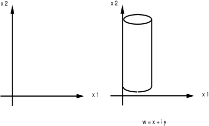
Figure 4: Some of the geometries used in the text.

From this, it follows that

$$\left<:e^{i\beta\Phi(w,\bar{w})}:\ :e^{-i\beta\Phi(w^{\prime},\bar{w}^{\prime})}:\right>_{cylinder}=\left({\pi T\over|\sin\pi T(w-w^{\prime})|}\right)^{\beta^{2}/2\pi}$$ (41)

Let us focus on the holomorphic part

$$\left<:e^{i\beta\phi(w)}:\ :e^{-i\beta\phi(w^{\prime})}:\right>_{cylinder}=\left({\pi T\over\sin\pi T(w-w^{\prime})}\right)^{\beta^{2}/4\pi}$$ (42)

This can be shown to be, equivalently,

$$\left<:e^{i\beta\phi(w)}:\ :e^{-i\beta\phi(w^{\prime})}:\right>_{cylinder}=\left({dz\over dw}\right)^{h}\left({dz^{\prime}\over w^{\prime}}\right)^{h}\left<:e^{i\beta\Phi(z)}:\ :e^{-i\beta\Phi(z^{\prime})}:\right>_{plane},$$ (43)

where we used the mapping $z=e^{-2i\pi Tw}$. The latter formula expresses the covariance of the two point function under the conformal transformation. Another example of such covariance is provided by the derivative of the field

$$\left<\partial_{w}\phi(w)\partial_{w^{\prime}}\phi(w^{\prime})\right>=\left({dz\over dw}\right)\left({dz^{\prime}\over dw^{\prime}}\right)\left<\partial_{z}\phi(z)\partial_{z^{\prime}}\phi(z^{\prime})\right>,$$ (44)

where we suppressed mention of the geometry, which is implicit in the variables used.

Relations like (43,44) are well expected, since the gaussian action is, in fact, conformal invariant; this follows, as discussed above, from the properties of the stress energy tensor, and thus is expected to generalize to other local massless field theories. More directly, this invariance is easily established for the free boson, since upon changing the argument of the field from $z\to w$ in the action, $S$ is invariant, the Jacobian cancelling the term coming from the partial derivatives.

Of course, one has to be quite careful in using the conformal invariance of the action, since the correlators are not invariant - ie, one has for instance, $\left<\Phi(w,\bar{w})\Phi(w^{\prime},\bar{w}^{\prime})\right>\neq\left<\Phi(z,\bar{z})\Phi(z^{\prime},\bar{z}^{\prime})\right>$, while the naive change of variables in the action would suggest the propagators to map straightforwardly, and thus the equality to hold. The reason for this discrepancy comes from the cut-off, which is also modified in a conformal transformation. We, on the other hand, wish to use the same regularization whatever the geometry, ie, for instance, use a square lattice of constant $a$ to regularize both the problem in the plane and on the cylinder; hence, there is an “anomaly”.

Fields obeying the general covariance relation (and a similar one for the antiholomorphic part)

$$\left<O(w)O(w^{\prime})\right>=\left({dz\over dw}\right)^{h}\left({dz^{\prime}\over dw^{\prime}}\right)^{h}\left<O(z)O(z^{\prime})\right>$$ (45)

are called primary fields. The field $\phi$ itself is not primary, though, in a way, it satisfies the equivalent of the previous relation with $h=0$, since

$$\left<\phi(w)\phi(w^{\prime})\right>=\left<\phi(z)\phi(z^{\prime})\right>+{1\over 8\pi}\ln\left({dz\over dw}{dz^{\prime}\over dw^{\prime}}\right)$$ (46)

Fields which are not primary exhibit in general more complicated covariance relations. An example is provided by the second derivative of $\phi$, which we leave to the reader to work out. A more interesting example is furnished by the stress energy tensor. Though we have defined it so far by normal ordering, it is clear that an equally good definition is obtained by point splitting, ie

$$T(z)=-2\pi\lim_{d\to 0}\left[\partial\phi(z+d/2)\partial\phi(z-d/2)+{1\over 4\pi d^{2}}\right]$$ (47)

We have thus, from the change of variables

$$T(z)=-2\pi\lim_{d\to 0}\left[w^{\prime}(z+d/2)w^{\prime}(z-d/2)\partial_{w}\phi(w(z+d/2))\partial\phi(w(z-d/2))-{1\over 4\pi d^{2}}\right]$$

To define the stress energy tensor on the cylinder, we use the same definition (47), but with $z$ replaced by $w$ . Therefore

$$T(z)=\left[w^{\prime}(z)\right]^{2}T(w)+{1\over 12}\{w,z\},$$ (48)

where the added term is

$${1\over 12}\{w,z\}=\lim_{d\to 0}{1\over 2}{w^{\prime}(z+d/2)w^{\prime}(z-d/2)\over[w(z+d/2)-w(z-d/2)]^{2}}-{1\over 2d^{2}}$$

This is known under the name of Schwartzian derivative, and reads

$$\{w,z\}={2w^{\prime\prime\prime}w^{\prime}-3w^{\prime 4}\over 2w^{\prime 2}}$$ (49)

It enjoys nice properties under the composition of successive conformal transformations, that we leave to the reader to investigate. An important property following from (48) is that $T$ acquires a finite expectation value on the cylinder, while it did not have one in the plane

$$\left<T\right>_{cylinder}=-{c\over 24}\left(2\pi T\right)^{2}$$ (50)

Exercise: show this by using the propagators on the plane and the cylinder, together with appropriate definitions of normal ordering.

The OPE of the stress energy tensor with any field of the theory has the general form

$$T(z)O(0,0)=\ldots+{h\over z^{2}}O(0,0)+{1\over z}\partial O(0,0)+\ldots$$ (51)

The two terms explicitely written follow from the fact that $O$ has dimension $h$ and the use of the Ward identity (57). It can be shown that $1/z^{2}$ is the highest singularity if $O$ is primary.

Exercise: check this for the free boson by considering various examples.

1.5 Some remarks on Ward identities in QFT.

Suppose in general that there is a transformation of the field $\Phi^{\prime}(x_{1},x_{2})=\Phi(x_{1},x_{2})+\delta\Phi(x_{1},x_{2})$ that leaves the product of the path integral measure and the Boltzmann weight $e^{-S}$ invariant. Examples of such transformations are provided for instance by translations or rotations in ordinary isotropic homogeneous physical systems. Consider then a transformation $\Phi^{\prime}(x_{1},x_{2})=\Phi(x_{1},x_{2})+\rho(x_{1},x_{2})\delta\Phi(x_{1},x_{2})$. For general $\rho$, this is not a symmetry of the problem anymore. On the other hand, we can always change variables in the functional integral and reevaluate any correlator in terms of the new field $\Phi^{\prime}$. This means that we have the identity

$$0=\int[d\Phi^{\prime}]e^{-S^{\prime}}-\int[d\Phi]e^{-S}$$ (52)

where in $S^{\prime}$ one maybe had to add up terms coming from the change of variables in the path integral. On the other hand, one can expand the right hand side of this equation to first order in the change of fields assumed small. Since for $\rho$ a constant the product of the measure and the weight would be invariant, this means that the right hand side of (52) must depend on the gradient of $\rho$ only, ie one has

$$\hbox{rhs= }{i\over 2\pi}\int[d\Phi]e^{-S}\int j_{\mu}\partial_{\mu}\ \rho dx_{1}dx_{2}$$ (53)

The quantity $j_{\mu}$ is called a Noether current. Since it comes from local manipulations, it must be a local quantity. Now, that (53) vanishes is something that must hold for any reasonably smooth function $\rho$. Let us choose $\rho$ to be equal to unity inside a disk of radius $R_{1}$, and to vanish on and outside of $R_{2}$, while it is arbitrary in between. Integrating (53) by parts, we get an integral of $j_{\mu}$ on the circle $R_{1}$, together with an integral on the annulus between $R_{1}$ and $R_{2}$ of $\partial_{\mu}j_{\mu}$. Since the functions $\rho$ is quite arbitrary there, it follows that the current has to be conserved, that is

$$\partial_{\mu}j_{\mu}=0$$ (54)

This result would still hold of course with fields inserted far from $R_{1}$ and $R_{2}$, so (54) truly holds as an operator equation, in the sense explained above.

As an application, consider a translation $x_{\mu}\to x_{\mu}+\epsilon_{\mu}$, where $\epsilon_{\mu}$ is small and constant: we obtain a current which, in the classical case, coincides with $ij_{\mu}=T_{\mu\nu}\epsilon_{\nu}$. The foregoing procedure is a generalization to the quantum theory, and the conservation equation follows from Noether’s theorem.

Now consider some field $O$ inside the circles, say right at the origin. Under the transformation $\Phi\to\Phi^{\prime}$, this field becomes $O^{\prime}=O+\delta O$ (the change is expanded to first order as before, but of course $O^{\prime}$ might as well depend on the derivatives of $\rho$ in general). We now have, since all we are doing is changing variables in the path integral

$$0=\int[d\Phi^{\prime}]O^{\prime}\ e^{-S^{\prime}}\ldots-\int[d\Phi]O\ e^{-S}\ldots$$ (55)

Expand this to first order. This time, the integration by part gives

$$-i\delta O={1\over 2\pi}\int(dx_{2}j_{1}-dx_{1}j_{2})O(0,0)={1\over 2i\pi}\int(dzj-d\bar{z}\bar{j})O(0,0)$$ (56)

As an application, consider a transformation $z\to z+\alpha(z)$. where $\alpha$ is small. The Noether current associated with it is given by $j=i\alpha(z)T(z)$ and $\bar{j}=i\bar{\alpha}(\bar{z})\bar{T}(\bar{z})$. For a transformation that is conformal inside a contour $C$, and differentiably connected to a (necessary non conformal) transformation vanishing at large distances, one finds from (56) the key result

$$\delta O={1\over 2i\pi}\int_{C}\alpha(z)T(z)O(0)dz-{1\over 2i\pi}\int_{\overline{C}}\bar{\alpha}(\bar{z})\bar{T}(\bar{z})O(0)d\bar{z}$$ (57)

Exercise: derive from this (51) and the fact that there are no singularities stronger than $1/z^{2}$ for a primary operator.

Notice finally that for the free boson, the expression of the stress energy tensor is almost the classical one, up to normal ordering, and it appears as if the integration measure essentially plays no role in the construction of the Ward identities. That one can forget about the behaviour of the measure in conformal transformations is justified a posteriori, by the fact that the quantum currents are indeed conserved. The measure would play a more subtle role for theories defined on curved two-dimensional manifolds.

1.6 The Virasoro algebra: intuitive introduction

As noticed before, the main consequence of conformal invariance is the existence of a conserved current, the stress energy tensor $T$. In general, one sets

$$T(z)=\sum_{n=-\infty}^{\infty}{L_{n}\over z^{n+2}}$$ (58)

that is, plugging this expansion into the OPE provides a definition of what the field $L_{n}O$ actually is: for instance $L_{0}O=hO$, $L_{-1}O=\partial O$, $L_{2}T=1$, etc. In general, one does not expect fields with negative dimensions to appear, or at least not fields with arbitrarily large negative dimensions (weird things can occur in non unitary theories adapted to disordered systems in particular though). This means that for every field, $L_{n}O$ must vanish for $n$ positive large enough. Of particular interest are the primary fields, for which the highest singularity is $1/z^{2}$, ie they satisfy $L_{n}O=0,n>0$.

For the moment, we can contend ourselves with the intuitively reasonable notion that the $L_{n}$ are “operators” acting on the space of fields of the theory - here, exponentials multiplied by normal ordered polynomials in derivatives of the field $\Phi$ - so the $L_{n}$ are not unlike differential operators acting on functions (in fact, the $(L_{-1})^{n}$ are just that).

It is then tempting to ask oneself what the algebra of these operators is, that is how do $L_{n}(L_{m}O)$ compare with $L_{m}(L_{n}O)$? This is easily done by using contour integration together with the short distance expansions. The commutator $[L_{n},L_{m}]O$ can be computed as follows. We have

$$L_{n}L_{m}O=\int_{C^{\prime}}{dz\over 2i\pi}z^{n+1}T(z)\int_{C}{dw\over 2i\pi}w^{m+1}T(w)O(0)$$ (59)

where the contours encircle the origin and $C$ is inside $C^{\prime}$ (see figure 5).

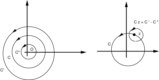
Figure 5: The contour manipulations that lead to the definition of a commutator in radial quantization.

Indeed, imagine writing the OPE of the integrand. First we expand $T(w)O(0)$ to extract the field $L_{m}O$, on which the action of $L_{n}$ is then obtained by the second integration. That the countour $C$ is inside $C^{\prime}$ is natural from the point of view of “radial quantization” which, as we will see later, gives a precise operatorial definition to the $L_{n}$’s. It is also necessary if one wishes to use the OPE in the order we just said for convergence reasons. The product $L_{m}L_{n}O$ is computed in the same fashion with this time with a contour $C^{\prime\prime}$ inside $C$: this forces one to expand first the product $T(z)O$, resulting in the opposite order for the operators. Comparing the two, and forgetting the operator $O$ itself, we see that

$$[L_{n},L_{m}]=\int_{C}{dz\over 2i\pi}\int_{C_{z}}{dw\over 2i\pi}z^{n+1}w^{m+1}T(z)T(w)$$ (60)

and a computation using the OPE of $T$ with itself gives

$$[L_{n},L_{m}]=(n-m)L_{n+m}+{c\over 12}(n^{3}-n)\delta_{n+m}$$ (61)

This is the celebrated Virasoro algebra, the $L_{n}$ being called Virasoro generators. It is an infinite dimensional Lie algebra.

Exercise: compute the action of the Virasoro generators of say derivatives of the field $\phi$, and directly check the Virasoro commutation relations.

A very important use of this algebra is to provide one with a natural structure to organize and recognize the fields in a theory. Of course, one does not quite need this powerful tool for the free boson, whose fields are easily built “by hand”, but for more complex theories, this is really very useful. Given a lattice model with microscopic variables, arbitrary combinations of neighbour variables can be built, whose scaling limit may or may not give rise to new scaling fields: which are truly new, which are nothing but “$L_{n}$”’s (descendents) of others? What happens is that a theory has a certain number of primary fields, which is very often finite (eg, three for the Ising model), and all the other fields are just descendents of these ones. The whole set of fields is thus organized into products of representations of the left and right Virasoro algebras, for which the primary fields are heighest weight states. This can be expressed by the compact form

$${\cal H}=\sum_{h,\bar{h}}Vir_{h}\otimes\overline{Vir}_{\bar{h}}$$ (62)

The situation is quite similar to the case of angular momentum in ordinary quantum mechanics, where the space of say the possible electronic states of some atom can be organized in terms of representations of the angular momentum algebra. Of course, here we have an algebra with an infinite number of generators, instead of three for angular momentum in three space dimensions. Qualitatively, there is an infinite number of Virasoro generators because there are an infinite number of elementary conformal transformations, one for each power of $z$: $z^{n}$.

As in the theory of angular momentum, unitarity contrains the quantum numbers, that is the values of conformal weights for a given central charge. This in turn gives rise to strong constraints for multipoint correlation functions; this is beyond the scope of these lectures, but not by far. In particular, correlations at strong coupling fixed points in the Kondo model can be computed just by using that technique [18].

The reason why we focused on the algebra of the $L_{n}$’s is because of the special role of the stress energy tensor in conformal transformations. Of course, we could define other operators and other algebras associated with any field that has an integer dimension (so the contour integrals can be closed in the complex plane. Generalizations also occur for fields with non integer, rational dimensions, and a cut plane, but this is more complicated). A natural candidate in condensed matter is provided by currents, for instance $\partial\phi$. Set therefore

$$i\partial\phi={1\over\sqrt{4\pi}}\sum_{n}{\alpha_{n}\over z^{n+1}},\ i\bar{\partial}\bar{\phi}={1\over\sqrt{4\pi}}\sum_{n}{\bar{\alpha}_{n}\over\bar{z}^{n+1}}$$ (63)

From

$$\left<\partial\phi(z)\partial\phi(w)\right>={1\over 4\pi}{1\over(z-w)^{2}},$$ (64)

it follows that

$$[\alpha_{n},\alpha_{m}]=n\delta_{m+n}$$ (65)

Here we recognize the oscillator algebra standard in the quantization of the free boson, and maybe it is time to discuss more what the mode expansion has to do with hamiltonian quantization.

1.7 Cylinders

I shall mostly discuss what happens in the case of the cylinder. The key idea here is to remember that path integrals are scalar products of states. If we insert a field $O$ at $y=-\infty$ on the cylinder, this corresponds to having prepared the system in a state (an “in” state) $\left|O\right>$, to which is associated, in the field representation a wave function $\Psi_{O}[\Phi_{S^{1}}]$, result of a partial path integration

$$\Psi_{O}[\Phi_{S^{1}}]=\int_{\Phi_{S^{1}}\ fixed}[d\Phi_{\Omega}]O(-\infty)\ e^{-S_{\Omega}}$$ (66)

where the integral is taken over all configurations of the field in the bottom part of the cylinder $\Omega=(-\infty,0]\times S^{1}$, the values at the boundary $S^{1}$ being held to $\Phi_{S^{1}}$ . Similarly if we insert a field $O^{\prime}$ at $\infty$, this corresponds to projecting the system on an “out” state $\left|O^{\prime}\right>$, to which is associated a wave fucntion $\Psi_{O^{\prime}}(\Phi_{S^{1}})$. The scalar product of these two states is then

$$\left<O|O^{\prime}\right>=\int[d\Phi_{S^{1}}]\Psi_{O^{\prime}}^{*}(\Phi_{S^{1}})\Psi_{O}(\Phi_{S^{1}}),$$ (67)

and this is essentially the correlation function of the two fields $O,O^{\prime}$. Of course, by translation invariance on the cylinder, this does not depend on the particular place where we have cut open the path integral.

To make things concrete, let us discuss an example we will use explicitly later, with $O=O^{\prime}=I$, the identity operator - ie, nothing is actually inserted at $\pm\infty$. In this case, (67) is just the partition function $Z$ of the problem. To find the wave functions, let us split open the path integral at $y=0$, and let us Fourier decompose

$$\Phi_{S^{1}}(x)=\sum_{n}\Phi_{n}e^{i\omega_{n}x},$$ (68)

where $\omega_{n}=2\pi nT$. Introduce then the solution of the Laplace equation $\Delta\Phi_{0}=0$ subject to the constraint $\Phi_{0}(x,y=0)=\Phi(x)$. One finds easily

$$\Phi_{0}(x,y)=\sum_{n}\Phi_{n}e^{-|\omega_{n}y|}e^{i\omega_{n}x}$$ (69)

We can now split the field in the path integral into $\Phi=\Phi_{0}+\Phi^{\prime}$ where $\Phi^{\prime}$ vanishes at $y=0$. Because of this, together with the fact that $\Phi_{0}$ solves Laplace equation, integration by parts shows that the path integral factorizes into the partition fucntions of two half cylinders with Dirichlet boundary conditions (we will get back to these later; the point here is that they are independent of $\Phi_{S^{1}}$), and an interesting term

$$Z=Z_{D}^{2}\int[d\Phi_{S^{1}}]\exp\left(-{1\over T}\sum_{n}|\omega_{n}||\Phi_{n}|^{2}\right)$$ (70)

Comparing with (67), it follows that, up to a phase

$$\Psi_{I}\left[\Phi_{S^{1}}\right]\propto\exp\left[-{\pi T^{2}\over 2}\int_{S^{1}}\left({\Phi(x)-\Phi(x^{\prime})\over\sin\pi T(x-x^{\prime})}\right)^{2}\right]$$ (71)

where we Fourier transformed back the integrand in (70).

We notice here as a side remark that the issue of finding wave functions is more than formal: the computation above was carried out for instance by people interested in finding the wave function of the Thirring model in terms of the original fermions [25].

In this point of view, we have a Hilbert space made up of states in one to one correspondence with the various fields of the theory. For operators other than the identity, one has to be a little bit careful. While the in state is always obtained by inserting $O$ at $-\infty$, the out state is obtained actually by inserting $\left(e^{-2i\pi Tw}\right)^{2h}\left(e^{-2i\pi T\bar{w}}\right)^{2\bar{h}}O$ at $+\infty$.

The same analysis can be carried out in the plane in the framework of “radial quantization”, where time is $\ln|z|$. This is why the expansions we used earlier were called OPE. To be correct however, they do have a meaning as OPE’s only when the operators are radially ordered, since recall that, to an Euclidian Green function computed with a path integral, there corresponds a time ordered Green function in the quantum field theory. Of course, other hamiltonian descriptions (for instance, the standard one where imaginary time runs say along $x_{2}$) could be obtained by splitting open the path integrals differently.

The remarkable thing now is, that the hamiltonian on the cylinder has a very simple spectrum. Indeed, first observe that for primary operators, using the formula (43), the two point function on the cylinder decreases at large distance along the cylinder as

$$\left<O(w)O(w^{\prime})\right>\approx\exp\left[-{2\pi T}(h+\bar{h})(y-y^{\prime})\right]\exp\left[-2i\pi T(h-\bar{h})(x-x^{\prime})\right]$$ (72)

For non primary operators, the same can be shown to hold, the more complicated terms in the covariance formula decreasing more quickly.

On the other hand, suppose we want to describe the theory on the cylinder in a hamiltonian formalism with imaginary time along the $y$ axis. As is well known, the rate of decay of correlation functions is given by the gaps of the hamiltonian, and the decay (72) indicates that there is an eigenstate of the hamiltonian whose eigenenergy is $2\pi T(h+\bar{h})$ over the ground state. More generally, the computation of any physical property of the theory boils down to evaluating correlators, which all obey (72): therefore, the whole space of the quantum field theory must be organized in states associated with the various observables, such that their eigenenergy is $2\pi T(h+\bar{h})$ over the ground state! This is exactly what we expected from the hamiltonian formalism described before, with one additional piece of information: the spectrum of $H$.

In addition, it is important to stress that the stress tensor acquires a non vanishing expectation value on the cylinder, due to the schwartzian derivative (50) . As a result, the hamiltonian on the cylinder reads

$$H=2\pi T\left(L_{0}+\bar{L}_{0}-{c\over 12}\right)$$ (73)

and the momentum

$$P=2\pi T\left(L_{0}-\bar{L}_{0}\right)$$ (74)

where $L_{0}$ has eigenvalues $h$, $\bar{L}_{0}$ eigenvalues $\bar{h}$.

We can of course define the whole set of Virasoro generators on the cylinder by

$$T(w)=(2\pi T)^{2}\left(\sum_{n}L_{n}e^{-2i\pi nTw}-{c\over 12}\right)$$ (75)

Now we have a precise meaning to give the $L_{n}$ as operators, and their commutator can be computed, of course giving rise to the same Virasoro algebra derived more intuitively before. Notice the identity

$$H={1\over 2\pi}\int_{0}^{1/T}(T+\bar{T})dx$$ (76)

This is independent of $x$, a result of analyticity.

It should be clear that the whole conformal invariance analysis could be written within the hamiltonian formulation. For instance, the OPE of $T$ with itself corresponds to the commutator

$${1\over 2i\pi}\left[T(x),T(x^{\prime})\right]=\delta(x-x^{\prime})T^{\prime}(x)-2\delta^{\prime}(x-x^{\prime})T(x)+{c\over 6}\delta^{\prime\prime\prime}(x-x^{\prime}),$$ (77)

and the OPE of $T$ with a primary field

$${i\over 2\pi}\left[T(x),O(x^{\prime})\right]=\delta(x-x^{\prime})\partial_{x}O-\delta^{\prime}(x-x^{\prime})hO$$ (78)

1.8 The free boson via hamiltonians

We now discuss the hamiltonian formalism more specifically for the free boson. The Lagrangian is

$$L={1\over 2}\int_{0}^{1/T}dx\left[\left(\partial_{t}\Phi\right)^{2}-\left(\partial_{x}\Phi\right)^{2}\right]$$ (79)

from which the momentum follows

$$\Pi=\partial_{t}\Phi$$ (80)

and the standard hamiltonian

$$H={1\over 2}\int_{0}^{1/T}\left[\Pi^{2}+\left(\partial_{x}\Phi\right)^{2}\right]$$ (81)

with the canonical equal time commutation relations

$$\left[\Phi(x,t),\Pi(x^{\prime},t)\right]=i\delta(x-x^{\prime})$$ (82)

The field is periodic in the space direction, that is $\Phi(x,t)\equiv\Phi(x+1/T,t)$. We chose to compactifiy the field on a circle of radius $r$, that is we identify $\Phi\equiv\Phi+2\pi r$. The mode expansion of the field reads then (see eg [26] for many more details on this)

$$\Phi(x,t)=\hat{x}+T\hat{p}t+2\pi Trwx+{i\over\sqrt{4\pi}}\sum_{n\neq 0}{1\over n}\left(\alpha_{n}e^{2i\pi Tn(x-t)}-\bar{\alpha}_{-n}e^{2i\pi Tn(x+t)}\right),$$ (83)

where $\hat{x}=T\int\Phi(x,t)dx=\Phi_{0}$ is the boson zero mode, while $\hat{p}=\int\Pi(x,t)dx=\Pi_{0}$ is the total momentum. $w$ in an integer (the winding number); $\hat{p}$ is quantized such that $r\hat{p}=k$ is also an integer. The commutation relations of the operators are $[\hat{x},\hat{p}]=i$ and

$$\left[\alpha_{n},\alpha_{m}\right]=\left[\bar{\alpha}_{n},\bar{\alpha}_{m}\right]=n\delta_{n+m},\ \left[{\alpha}_{n},\bar{\alpha}_{m}\right]=0$$ (84)

The operators $\alpha_{n},\bar{\alpha}_{n}$ are related with the usual creation and annihilation operators of the free boson harmonic oscillators by

$$\alpha_{n}=-i\sqrt{n}a_{n},n>0,\ \alpha_{n}=i\sqrt{-n}a_{-n}^{\dagger},n<0$$ (85)

and

$$\bar{\alpha}_{n}=-i\sqrt{n}\bar{a}_{-n},n>0,\ \bar{\alpha}_{n}=i\sqrt{-n}\bar{a}_{n}^{\dagger},n<0$$ (86)

Note that if we go to euclidian space time, replacing $t$ by $-iy$ and then use the conformal coordinates $z=e^{2\pi T(y-ix)}$ ($z=e^{-2i\pi Tw}$, $\bar{z}=e^{2\pi T(y+ix)}$), we obtain the expansion

$$\Phi(z,\bar{z})=\Phi_{0}-i\left({\hat{p}\over 4\pi}+{wr\over 2}\right)\ln z-i\left({\hat{p}\over 4\pi}-{wr\over 2}\right)\ln\bar{z}+{i\over\sqrt{4\pi}}\sum_{n\neq 0}{1\over n}\left(\alpha_{n}z^{-n}+\bar{\alpha}_{n}\bar{z}^{-n}\right)$$ (87)

When the winding number is non zero, the field is not periodic around the origin; rather, a “vortex” is inserted there. When $w=0$, we can set $\alpha_{0}=\bar{\alpha}_{0}={\hat{p}\over\sqrt{4\pi}}$, one recovers the expansion (63) for $i\partial\phi$. In general, we will set

$$\alpha_{0}={\hat{p}\over\sqrt{4\pi}}+wr\sqrt{\pi},\ \bar{\alpha}_{0}={\hat{p}\over\sqrt{4\pi}}-wr\sqrt{\pi}$$ (88)

The hamiltonian (81) reads , before regularization

$$H=2\pi T\left[\pi(wr)^{2}+{\hat{p}^{2}\over 4\pi}+{1\over 2}\sum_{n\neq 0}\left(\alpha_{-n}\alpha_{n}+\bar{\alpha}_{-n}\bar{\alpha}_{n}\right)\right]$$ (89)

A question that arises now is the relation between the normal ordering defined in the field theory and the normal ordering in the usual sense of ordering free bosonic operators in quadratic expressions: $:\alpha_{n}\alpha_{m}:=\alpha_{inf(n,m)}\alpha_{sup(n,m)}$. The two might differ by a constant; in the present case actually, they coincide provided one uses zeta regularization. Indeed, by ordering $H$, we encounter a divergent term $\sum n$, which we can regularize by (for results on the zeta function, see [27])

$$\sum_{1}^{\infty}n=\zeta(-1)=-{1\over 12}$$ (90)

With this prescription, the hamiltonian with the vacuum energy divergence subtracted reads as it should (73), with the Virasoro generators

$$L_{n}={1\over 2}\sum_{m}\alpha_{n-m}\alpha_{m},\ \bar{L}_{n}={1\over 2}\sum_{m}\bar{\alpha}_{n-m}\bar{\alpha}_{m}$$ (91)

together with

$$L_{0}={1\over 2}\alpha_{0}^{2}+\sum_{n=1}^{\infty}\alpha_{-n}\alpha_{n},\ \bar{L}_{0}={1\over 2}\bar{\alpha}_{0}^{2}+\sum_{n=1}^{\infty}\bar{\alpha}_{-n}\bar{\alpha}_{n}$$ (92)

The modes $\alpha_{n}$ and $\bar{\alpha}_{n}$ are annihilation operators for $n>0$ and creation operators for $n<0$. The whole space of fields is thus obtained starting from highest weight states $\left|w,k\right>$ which are annihilated by the annihilation operators and are eigenstates of the zero modes, and applying creation operators to them. Schematically, one has

$${\cal H}=\sum_{w,k}Heis_{w,k}\otimes\overline{Heis}_{w,k}$$ (93)

Of course, the $\left|w,k\right>$ states are primary, and thus highest weight of the Virasoro algebra. Accordingly, one could as well build the whole space of fields by acting on them with $L_{n}^{\prime}s$. This would be more complicated; for instance, the field $\partial\phi$, which is simply the result of $\alpha_{-1}\left|0,0\right>$, is not obtained from the action of $L_{-1}$ on that state at all. This means in general that more primary fields are necessary than the $\left|w,k\right>$ in the Virasoro description.

1.9 Modular invariance

A convenient way of encoding the field content of the theory is to write the torus partition function, that is, the partition function when one imposes periodic boundary conditions in the imaginary time direction, too. One has, using (73)

$$Z=\hbox{Tr }\exp\left[-{2\pi TL}\left(L_{0}+\bar{L}_{0}-{c\over 12}\right)\right]$$ (94)

Using the mode decomposition, one finds easily

$$Z={1\over\eta(q)\bar{\eta}(\bar{q})}\sum_{w,k}q^{h_{wk}}\bar{q}^{\bar{h}_{wk}}$$ (95)

where $q=e^{-2\pi TL}=\bar{q}$ (the notation allows consideration of more complicated parallelograms),

$$\eta(q)=q^{1\over 24}\prod_{n=1}^{\infty}(1-q^{n})$$ (96)

and

$$h_{wk}=2\pi\left({k\over 4\pi r}+{wr\over 2}\right)^{2},\ \bar{h}_{wk}=2\pi\left({k\over 4\pi r}-{wr\over 2}\right)^{2}$$ (97)

An important property of this partition function is that it is modular invariant. What this means is, suppose one considers quantization of the free boson with time in the $x$ instead of $y$ direction. The radius being the same, this will lead to the same expression as (95) but with $L$ and $1/T$ exchanged, that is

$$Z={1\over\eta(q^{\prime})\bar{\eta}(\bar{q}^{\prime})}\sum_{w,k}\left(q^{\prime}\right)^{h_{wk}}\left(\bar{q}^{\prime}\right)^{\bar{h}_{wk}}$$ (98)

where $q^{\prime}=e^{-2\pi/TL}$. The expressions (95) and (98) do turn out to be equal thanks to some elliptic functions identities (see next section). They ought to be, of course, since they represent the same physical object from two different points of view.

For more sophisticated theories, the partition function cannot be computed a priori, but it is possible to determine it by imposing that it does not depend on the description, ie is modular invariant. See [22] and references therein for more details.

2 Conformal invariance analysis of quantum impurity fixed points

2.1 Boundary conformal field theory

An excellent reference for this part is the original work of J. Cardy ([28]). Consider now a field theory defined only on the half plane $x_{2}>0$ (figure 6) - it might be for instance the continuum limit of a 2D statistical mechanics model which is at its critical point in the bulk, that is $T=T_{c}$, the usual critical temperature of the system. Various situations could occur at the boundary depending on whether the coupling there is enhanced, or whether some quantum boundary degrees of freedom have been added.

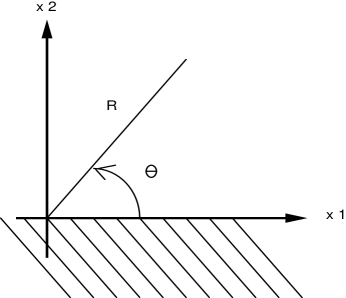
Figure 6: The geometry for boundary conformal field theory.

Consider, to fix ideas, the simplest case where the statistical mechanics model would have the same couplings in the bulk and the boundary ( the so called “ordinary transition”). Intuitively, one expects the system to still be invariant under global rotations, dilations and translations that preserve the boundary, and that this invariance should be promoted to a local one, ie conformal invariance in the presence of the boundary.

Physical fields are now characterized both by a bulk and a boundary anomalous dimension. If both fields are taken deep inside the system, they behave as in the bulk case. On the other hand, if they are near the boundary, one has, for example,

$$\left<O(x_{1},x_{2})O(x^{\prime}_{1},x^{\prime}_{2})\right>\approx{1\over|x_{1}-x^{\prime}_{1}|^{2d_{s}}},~{}~{}~{}|x_{1}-x^{\prime}_{1}|>>x_{2},x_{2}^{\prime}$$ (99)

ie the large distance behaviour of the correlators parallel to the surface is determined by the boundary dimension. We quote also the formula

$$\left<O(x_{1},x_{2})O(x^{\prime}_{1},x_{2}^{\prime})\right>\approx{1\over R^{d+d_{s}}}\left(\cos\theta\right)^{d_{s}-d}$$ (100)

A condition of boundary conformal invariance is that $T_{12}=T_{21}=0$ when $x_{2}=0$, which means physically that there is no flux of energy through the boundary. As a result, the left and right components of the stress tensor are not independent anymore, but $T=\bar{T}$ for $Imz=0$; this is expected, since the theory is invariant only under the transformations that preserve this boundary, that is satisfy $w=\bar{w}$ for $Imz=0$. As a result however, one can define formally the stress tensor in the region $Imz<0$ by setting

$$T(z)=\bar{T}(z),\ Imz<0$$ (101)

Instead of having a half plane with left and right movers, we can thus equivalently describe the problem with only right movers on the full plane.For instance, the two point correlation function in the half plane is related with the four point correlation function in the full plane. Also radial quantization corresponds to propagating outwards from the origin in the upper half plane, with hamiltonian (see figure 7)

$$\int_{C}T(z)dz+cc$$ (102)

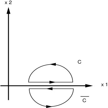
Figure 7: Geometry of the contours for the boundary case.

Using the continuation (101), this becomes a closed contour integral of $T$ only: thus, the Hilbert space of the theory with boundary is described by a sum of representations of a single Virasoro algebra this time:

$${\cal H}=\sum_{h}Vir_{h}$$ (103)

The natural mapping in this problem is $w=-{L\over i\pi}\ln z$, which maps the half plane onto a strip of width $L$ with the same boundary conditions on both sides . The hamiltonian now reads

$$H={\pi\over L}\left(L_{0}-{c\over 24}\right)$$ (104)

Note that there are, roughly, two factors of two differing from the periodic hamiltonian: the prefactor has a $\pi$ instead of $2\pi$, and there is a single Virasoro generator in the bracket. The space onto which the periodic hamiltonian (73) acts is uniquely defined by the (bulk) theory one is dealing with, say the Ising model - as we discussed, this specification amounts to giving the various representations of $Vir\ \otimes\ \overline{Vir}$ defining the model. For (104), the space depends on the boundary conditions; it is specified by a set of representations of a single Virasoro algebra. By a careful study of the two point function in the plane, together with the conformal transformation (where the jacobians still involve the bulk dimension), one can show that the gaps of $H$ are given by the corresponding surface dimensions.

It is important to stress again that the same physical obervable will be associated with different representations of the Virasoro algebra in the bulk and boundary cases. For instance, the spin in the Ising model coresponds, in the bulk, to $Vir_{1/16}\otimes\overline{Vir}_{1/16}$, while with free boundary conditions, it corresponds to $Vir_{1/2}$ (with fixed boundary conditions, the spin is the same as the identiy operator).

2.2 Partition functions and boundary states

To classify boundary conditions, it is extremely useful to deal with partition functions a bit. We consider thus a cylinder with a periodic direction of length $1/T$ and a non periodic one of length $L$: on either side, boundary conditions of type $a,b$ have been imposed. We can describe the situation in two ways (see figure 8): either imaginary time runs in the direction parallel to the boundary (“open channel”), in which case we can write the partition function as

$$Z=Tre^{-H_{ab}/T}$$ (105)

where $H_{ab}$ is the hamiltonian (104) with boundary conditions $a$ and $b$, or imaginary time can run in the direction perpendicular to the boundary (“closed channel”), in which case

$$Z=\left<B_{a}|e^{-LH}|B_{b}\right>$$ (106)

where $\left|B_{a}\right>,\left|B_{b}\right>$ are boundary states, and $H$ is the periodic hamiltonian (73).

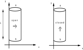
Figure 8: The open and closed channel geometries when boundaries are present.

Observe that the the boundary states are not normalized: they are entirely determined, including their norm, by the condition that (106) gives the right partition function. To make things more concrete, fixed boundary conditions in the Ising model for instance are represented, in the microscopic Hilbert space, by the state $\left|B\right>_{fixed}=\prod_{i}\left|+\right>$, while for free boundary conditions one has $\left|B\right>_{free}=\prod_{i}\left(\left|+\right>+\left|-\right>\right)$.

Here the boundary states are states in the Hilbert space of the bulk theory, ie in $Vir\ \otimes\ \overline{Vir}$. Conformal invariance at the boundary requires

$$\left(L_{n}-\bar{L}_{-n}\right)\left|B\right>=0$$ (107)

A solution to this equation is provided by so called Ishibashi states [30]

$$\left|h\right>=\sum_{n}\left|h,n\right>\otimes\left|\overline{h,n}\right>$$ (108)

where $\left|h,n\right>$ denotes an orthonormal basis of the representation $Vir_{h}$, and $\left|\overline{h,n}\right>$ the corresponding basis of $\overline{Vir}_{h}$.

In the case of the free boson, a boundary state will satisfy (107) if it satisfies a stronger constraint

$$\left(\alpha_{n}\pm\bar{\alpha}_{-m}\right)\left|B\right>=0$$ (109)

This in fact corresponds to Neumann and Dirichlet boundary conditions, for which $T_{12}\propto\partial_{1}\Phi\partial_{2}\Phi=0$. The negative sign in (109) is solved by

$$\left|B\right>\propto\exp\left[-\sum_{n=1}^{\infty}{\alpha_{-n}\bar{\alpha}_{-n}\over n}\right]\left|0,k\right>$$ (110)

Therefore, we can build boundary states by

$$\sum_{k}c_{k}\exp\left[-\sum_{n=1}^{\infty}{\alpha_{-n}\bar{\alpha}_{-n}\over n}\right]\left|0,k\right>$$ (111)

The question of interest is to determine the coefficients $c_{k}$. A quick way to proceed is to recognize here a Dirichlet state: indeed, suppose we act with $\Phi(x,t=0)$ on the boundary state. Because of the condition (109), the oscillator part just does not contribute; what does contribute is only the $\hat{x}$ part, which acts as $\hat{x}=i{\partial\over\partial p}$. Therefore, we have

$$\left|B_{D}(\Phi_{0})\right>={\cal N}_{D}\sum_{k=-\infty}^{\infty}e^{-ik\Phi_{0}/r}\exp\left[-\sum_{n=1}^{\infty}{\alpha_{-n}\bar{\alpha}_{-n}\over n}\right]\left|0,k\right>$$ (112)

The last question, which is actually of key importance for what follows, is the determination of the overall factor ${\cal N}$: in other words, what is the overall normalization of boundary states? This is where the consideration of partition functions is useful.

To answer this, we observe that, if we compute the partition function with height $\Phi_{0}$ on both sides, the identity representation should appear once and only once. On the other hand, the partition function is easily computed in the closed channel from the boundary states: one finds, for more general pair of values at the boundary

$$Z=\left<B_{D}(\Phi_{0})|e^{-LH}|B_{D}(\Phi^{\prime}_{0})\right>={\cal N}_{D}^{2}{1\over\eta(\tilde{q})}\sum_{k=-\infty}^{\infty}\tilde{q}^{k^{2}/8\pi r^{2}}e^{ki(\Phi_{0}-\Phi^{\prime}_{0})/r}$$ (113)

where $\tilde{q}=e^{-4\pi TL}$. We now perform a modular transformation to reexpress this partition function in terms of the other parameter $q=e^{-\pi/LT}$. One has (the proof of this is a bit intricate. See eg [29], chapter 3.)

$$\eta(\tilde{q})={1\over\sqrt{2TL}}\eta(q)$$ (114)

and, by using Poisson resummation formula for the infinite sum,

$$\sum_{n}\exp\left(-\pi an^{2}+bn\right)={1\over\sqrt{a}}\sum_{k}\exp-{\pi\over a}\left(k+{b\over 2i\pi}\right)^{2}$$ (115)

one finds

$$Z_{DD}=\sqrt{\pi}2r{{\cal N}_{D}^{2}\over\eta(q)}\sum_{n}q^{{1\over 2\pi}\left(\Phi_{0}-\Phi^{\prime}_{0}+2\pi nr\right)^{2}}$$ (116)

This expression has a simple interpretation: one sums over all the sectors where the difference of heights between the two sides of the cylinder is $\Phi_{0}-\Phi^{\prime}_{0}+2\pi rn$. For each such sector, the partition function is the product of a basic partition function corresponding to heights equal (without the $2\pi r$ identification) on both sides, times the exponential of a classical action. The latter is easily obtained: the classical field is $\Phi={\Phi_{0}-\Phi^{\prime}_{0}+2\pi nr\over L}y$, whose classical action is

$$\exp\left[-{1\over 2LT}(\Phi_{0}-\Phi^{\prime}_{0}+2\pi nr)^{2}\right]$$

Consider now (116). We know that the partition function must write as a sum of characters (that is, $Tr_{Vir_{h}}q^{L_{0}-c/24}$, as follows from (103) and (104)) of the Virasoro algebra with integer coefficients; even though I will not spend time discussing what the characters at $c=1$ are ($q^{h}/\eta$ for generic $h$), it is easy to see that this implies that the prefactor in (116) has to be an integer. Since we do not expect the normalization of the boundary states to change discontinuously with $\Phi_{0}$, this integer is actually a constant, whatever $\Phi_{0},\Phi_{0}^{\prime}$. We can in particular choose $\Phi_{0}=\Phi_{0}^{\prime}$, for which the identity representation $Vir_{h=0}$ appears in the spectrum; of course it should appear only once, and therefore

$${\cal N}_{D}={1\over\sqrt{2r\sqrt{\pi}}}$$ (117)

The other condition corresponds to Neumann boundary conditions, or, equivalently, Dirichlet boundary conditions on the dual field $\tilde{\Phi}=\tilde{\Phi}_{0}$. One finds the boundary state

$$\left|B_{N}(\tilde{\Phi}_{0})\right>={\cal N}_{N}\sum_{w=-\infty}^{\infty}e^{-2i\pi rw\tilde{\Phi}_{0}}\exp\left[\sum_{n=1}^{\infty}{\alpha_{-n}\bar{\alpha}_{-n}\over n}\right]\left|w,0\right>$$ (118)

The Neumann Neumann partition function reads then

$$Z_{NN}={1\over\eta(q)}\sum_{n}q^{{1\over 2\pi}\left(\tilde{\Phi}_{0}-\tilde{\Phi^{\prime}}_{0}+n/r\right)^{2}},$$ (119)

and one has

$${\cal N}_{N}={1\over 2}\sqrt{2r\sqrt{\pi}}$$ (120)

The Neumann Dirichlet partition function is actually independent of the values of $\Phi_{0},\tilde{\Phi}_{0}$, since then the field cannot wind in any direction.

Exercise: show the following

$$Z_{ND}={1\over 2\eta(q)}\sum_{n}q^{{1\over 4}(n-1/2)^{2}}.$$ (121)

The consideration of boundary states is extremely powerful to find out and study boundary fixed points. A general strategy is, knowing the Virasoro algebra symmetry of the model at hand, to try to find out combinations of Ishibashi states that are acceptable boundary states. Solving this problem involves rather complicated constraints. For instance, if one has several possible candidates $\left|B_{i}\right>$, the partition function with boundary conditions $ij$ can easily be evaluated in the closed channel; after modular transformation to the open channel, it should expand as a sum of characters of the Virasoro algebra with integer coefficients. Another constraint is that the identity representation should appear at most once in all open channel partition functions. Clearly, this becomes a rather technical subject; more details can be found in the paper of J. Cardy [32]. Questions like the completeness of boundary states (ie whether all the boundary fixed points of a given bulk problem are known) are still open in most cases.

2.3 Boundary entropy

Let us now suppose that we have a one dimensional quantum field theory defined on a segment of length $L$, with some boundary conditions at $x=0$ and $x=L$. As is well known, the partition function at temperature $T$ of this theory will be given by the same expression as the partition function of the two dimensional systems considered previously; notice however that I have changed conventions calling now $x$ (resp. $y$) what was $y$ (resp. $x$) previously (see figure 9) .

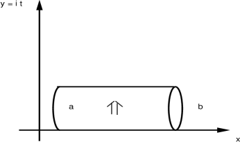
Figure 9: The geometry for defining boundary entropy.

In terms of the parameter $q$, this partition function is expressed as a sum of terms ${q^{h}\over\eta}$ with integer coefficients: the spectrum of $H_{ab}$ is discrete, and its ground state has integer degeneracy, nothing very exciting. In the limit $L\to\infty$, the spectrum becomes gapless however, and one has to be more careful about the concept of degeneracy. If we take this limit, the free energy of the quantum field theory behaves as

$$F=-Lf+f_{a}+f_{b}$$ (122)

where $f$ is a free energy per unit length, $f_{a},f_{b}$ are boundary contributions. These contributions will involve, as $T\to 0$, a boundary energy that is non universal, but also a boundary entropy. It is easy to see what this entropy will be by using a modular transformation. The same partition function expresses then as a sum of ${\tilde{q}^{h}\over\eta(\tilde{q})}$ with some non integer coefficients that come from the Poisson resummation formula (in general, from the modular $S$ matrix). In the large $L$ limit, $\tilde{q}\to 0$. From the fact that

$$F=-T\ln Z$$ (123)

we see that, as $T\to 0$, $f=O(T^{2})$ (the ground state energy of $H_{ab}$ is set to zero in this approach; for the exact dependence of $f$ on $T^{2}$ see section 6), while $f_{a}$ and $f_{b}$ are of the form

$$f_{a}=-T\ln g_{a},f_{b}=-T\ln g_{b}$$ (124)

where [33]:

$$g_{a}=\left<B_{a}|0\right>,\ g_{b}=\left<0|B_{b}\right>$$ (125)

A one dimensional massless quantum field theory defined on a line with boundary conditions (or boundary degrees of freedom as we will see next) therefore has a non trivial zero temperature boundary entropy, or ground state degeneracy.

Exercise: Show that the precise meaning of this degeneracy is related with the behaviour of the density of states

$$D(n)\approx{g_{a}g_{b}\over 2}\left({c\over 6n^{3}}\right)^{1/4}\exp\left(2\pi\sqrt{cn\over 6}\right)$$ (126)

where we parametrized the excitation energies of $H_{ab}$ by $e_{n}={n\pi\over L}$, $n,L$ large (when computing the partition function and its logarithm, do not forget to integrate the fluctuations around the saddle point!).

As we have seen in the previous subsection, some boundary conditions have a degeneracy $g<1$, ie a negative boundary entropy. This is a bit shocking, but of course we should remember, first, that $g$ is more a prefactor in an asymptotic formula for degeneracies (126) than a true ground state degeneracy (at $L=\infty$, there is no gap), and second, that we are dealing with quantum field theories and that this is only a finite, properly regularized “entropy”. The same remark applies, somehow, to $g$ being non integer. However, it is perfectly possible to have non integer degeneracies for semi-classical systems involving kinks [34].

Intermezzo

Perturbation near the fixed points

A scale-invariant boundary condition is a RG fixed point (recall that the bulk is always critical in the type of systems that we are considering here). As with any RG fixed point, there is a set of relevant/marginal/irrelevant boundary operators (and couplings) associated with each scale-invariant boundary condition. These operators have support only at the boundary, i.e. at one point in position space (at the position of the impurity).

If no relevant boundary operators are allowed, then the scale invariant boundary condition represents a stable fixed point (the zero temperature fixed point, describing the Kondo model at strong coupling, is an example; so is the Dirichlet fixed point in the tunneling problem, to which we will get back soon). Irrelevant boundary operators give perturbatively calculable corrections to physical properties evaluated at the RG fixed point. Many important physical features of the Kondo model are actually due to the effect of the leading (dominant) irrelevant boundary operator [18].

Adding a relevant boundary operator to the Hamiltonian describing a particular scale-invariant boundary condition, destroys that boundary condition, and causes crossover to a new, scale-invariant boundary condition at large distances and low temperatures (in the infrared). In other words, we have a (boundary) RG flow, describing the crossover from the initial scale-invariant boundary condition (in the ultraviolet, i.e. at short distances or high temperatures) to a new scale invariant boundary condition (in the infrared, i.e. at large distances and low temperature).

Note that at every stage of this flow, the bulk remains always critical and unchanged; the only action is at the boundary. An interesting observation concerning general boundary RG flows was made in [33]: the zero-temperature boundary entropies ($s=\ln g$ in the previous section) generally obey

$$s_{UV}>s_{IR},\qquad{\rm(decrease\ of\ boundary\ entropy)}$$

This may be viewed as a boundary analogue of the well known $c$-theorem of bulk conformal field theory [35]. (Note, however, that the universal numbers $s_{UV}$ and $s_{IR}$ do not seem to be obviously related to a dynamical quantity, in contrast with the central charge, which is related to the stress tensor of CFT).

A well known example is the one-channel Kondo model. Initially, at weak coupling (at high temperature, in the ultraviolet), we have a quantum mechanical spin decoupled from the electron degrees of freedom of the metal. An isolated ($s=1/2$) spin has a zero-temperature entropy of $s_{UV}=\ln 2$. At strong coupling (at low temperature, in the infrared), this impurity spin is completely screened by the conduction electrons. This means that no dynamical degrees of freedom are left, and thus we have $s_{IR}=0$.

3 The boundary sine-Gordon model: general results

3.1 The model and the flow

We consider now the model we had decided to tackle in the introduction

$$S={1\over 2}\int_{-\infty}^{0}dx\int dy\left[\left(\partial_{x}\Phi\right)^{2}+\left(\partial_{y}\Phi\right)^{2}\right]+\lambda\int dy\cos{\beta\over 2}\Phi(0,y).$$ (127)

This model is called the boundary sine-Gordon model since it has a sine-Gordon type interaction, but at the boundary. In more general terms than those of the edge states tunneling, the physics of this model is rather clear. The limits $\lambda=0$ and $\lambda=\infty$ are fixed points, corresponding to conformal invariant boundary conditions, respectively of Neumann and Dirichlet types. Away from these limits, the model is not scale invariant because of the boundary interaction. In the vicinity of $\lambda=0$, the RG equation is

$${d\lambda\over db}=\left(1-g\right)\lambda+O(\lambda^{3}),$$ (128)

where we have set $g=\nu={\beta^{2}\over 8\pi}$. It is natural to expect that $\lambda$ flows all the way from $0$ to $\infty$ under renormalization. Equivalently, the boundary conditions look like Neumann at very high energy (UV) but like Dirichlet at low energy (IR) - the dimension of the physical coupling is $[\lambda]=L^{g-1}$, so the typical energy scale for the cross over between UV and IR behaviours is $T_{B}\propto\lambda^{1\over g-1}$. Equivalently also, the field $\Phi$ feels Neumann boundary conditions close to the boundary, but feels Dirichlet boundary conditions instead far from it, with a cross over distance $1/T_{B}$.

Notice that the boundary entropies of the UV and IR fixed points are different. To compute them, we can use the results of the previous section after having identified the radius of the boson. In the shift $\Phi\to\Phi+2\pi r$, the interaction $\cos{\beta\over 2}\Phi$ must be unchanged, which requires

$$r={2\over\beta}$$ (129)

It follows that

$$g_{N}=\left({\beta^{2}\over 4\pi}\right)^{-1/4},\ g_{D}=\left({\beta^{2}\over 16\pi}\right)^{1/4}$$ (130)

Notice the ratio

$${g_{N}\over g_{D}}=\left({\beta^{2}\over 8\pi}\right)^{-1/2}$$ (131)

For the case of a relevant perturbation we are considering here, this ratio is larger than one: the boundary entropy is greater in the UV than it is in the IR. This is in agreement with the intuitive idea that degrees of freedom disappear under the renormalization group, leading to a loss of information. There is a well known conjecture stating that for any allowed flow in a unitary system (that is, roughly, a system with real, local hamiltonian), $g_{UV}>g_{IR}$. For the case of irrelevant perturbation, one finds $g_{N}<g_{D}$, so according to this the flow should not be possible, which is indeed the case: since the operator is irrelevant, it does not generate any flow, and one should observe N boundary conditions both at small and large distance.

3.2 Perturbation near the UV fixed point

The first question we will be interested in is the calculation of the boundary free energy at any temperature $T$ and coupling $\lambda$. This can be represented by a Coulomb gas expansion as follows. First, by using a conformal mapping, one finds the two point function of the free boson with Neumann boundary conditions on the half cylinder

$$\left<\Phi(y)\Phi(y^{\prime})\right>=-g\ln\left|{\sin\pi T(y-y^{\prime})\over\pi T}\right|$$ (132)

Exercise: derive this, by first computing the two point function on the half plane.

We can then evaluate the ratio of partition functions with and without boundary interaction as follows

$${Z(\lambda)\over Z(\lambda=0)}=1+\sum_{n=0}^{\infty}{1\over(2n)!}\lambda^{2n}\int_{0}^{1/T}dy_{1}\ldots dy_{2n}\left<\cos{\beta\over 2}\Phi(y_{1})\ldots\cos{\beta\over 2}\Phi(y_{2n})\right>.$$ (133)

Of course, only electrically neutral configurations with $n$ positive and $n$ negative charges contribute. After some rescaling, one finds

$${Z(\lambda)\over Z(\lambda=0)}=1+\sum_{n=1}^{\infty}(\tilde{\lambda})^{2n}I_{2n},$$ (134)

where the dimensionless coupling is

$$\tilde{\lambda}={\lambda\over 2T}(2\pi T)^{g},$$ (135)

and the integrals are

$$I_{2n}={1\over(n!)^{2}}\int_{0}^{2\pi}du_{1}\ldots\int_{0}^{2\pi}du^{\prime}_{2n}\left|{\prod_{i<j}4\sin{u_{i}-u_{j}\over 2}\sin{u^{\prime}_{i}-u^{\prime}_{j}\over 2}\over\prod_{i,j}2\sin{u_{i}-u^{\prime}_{j}\over 2}}\right|^{2g}.$$ (136)

This is the partition function of a classical Coulomb gas in two space dimensions, with the charges moving on a circle of unit radius (see figure 10).

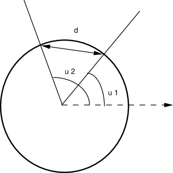
Figure 10: Charges of a two dimensional Coulomb gas that move on a circle $d=2\sin{u_{2}-u_{1}\over 2}$.

The integrands have small distance behaviours $1/u^{2g}$. It follows that there is no short distance divergence, and the integrals are all finite for $g<{1\over 2}$ (there are never large distance divergences here since we have a temperature). When $g>{1\over 2}$, the integrals have divergences. In the sequel, I will always regularize integrals dimensionally, not by introducing a cut-off. To explain what this means, consider the case $n=1$, which can be done by elementary computations

$$I_{2}={\Gamma(1-2g)\over\Gamma^{2}(1-g)}.$$ (137)

This can then be continued beyond $g={1\over 2}$ simply by using the known continuation of $\Gamma$ to negative arguments. How to do this in the case of arbitrary $n$ is a bit more tricky. A way to do it relies on the remarkable fact that the integrals $I_{2n}$ can be expressed in an almost closed form by appealing to techniques of Jack polynomials [36, 37]. I will only give the result here

$$I_{2n}={1\over[\Gamma(g)]^{2n}}\sum_{m}\prod_{i=1}^{n}\left({\Gamma[m_{i}+g(n-i+1)]\over\Gamma[m_{i}+g(n-i)+1]}\right)^{2}$$ (138)

where the sum is over all sets (Young tableaux) $m=(m_{1},\ldots,m_{n})$ with integers $m_{i}$ obeying $m_{1}\geq m_{2}\ldots\geq m_{n}\geq 0$. This expression can be used to compute the $I_{2n}$ numerically to high values of $n$, or, more fundamentally, to perform the analytic continuation in $g$. I will not discuss this further, and get back now to the physics of this model.

For $g<{1\over 2}$ at least, the perturbative expansion is well defined, giving a series in $\lambda$ with positive coefficients. This series will presumably have a finite radius of convergence - although one does not expect the appearance of a singularity on the positive real axis (this would correspond to the existence of a phase transition on the one dimensional boundary). Beyond this radius, some other technique has to be used to understand quantitatively what happens. It is possible to argue what the leading behaviour of the partition function at large $\lambda$ should be. Indeed, $Z$ actually depends only on the ratio of the two energy scales $T_{B}$ and $T$, so large $\lambda$ is like small temperature. But small temperature corresponds, going back to an euclidean description, to a cylinder of large diameter. In this limit, the partition function per unit length of the boundary should have a well defined, “thermodynamic” limit, so $Z$ should go as $Z\propto\exp\left({T_{B}\over T}\right)$. This means our perturbative series has to go as $\exp(cst\tilde{\lambda}^{1/1-g})$.

3.3 Perturbation near the IR fixed point

A natural idea to find out what happens beyond the radius of convergence is to think of the problem from a “dual” point of view, ie around the $\lambda=\infty$ infra red fixed point. The first question one may ask is along which irrelevant operator this fixed point is approached. There are several, equally interesting ways to answer this question.

The first one starts by considering the model where the bulk degrees of freedom have been integrated out, leading to the action (at zero temperature, which makes the formulas a bit simpler)

$$S={1\over 2\pi}\int dydy^{\prime}\left[{\Phi(y)-\Phi(y^{\prime})\over y-y^{\prime}}\right]^{2}+\lambda\int dy\cos{\beta\over 2}\Phi(y)+{m\over 2}\int dy\left(\partial_{y}\Phi\right)^{2}$$ (139)

where we have added an irrelevant mass term to make some integrals finite.

We can find kinks interpolating between adjacent vacua and satisfying the equations of motion [38]

$$m\partial^{2}_{y}\Phi=-{\lambda\beta\over 2}\sin{\beta\over 2}\Phi$$ (140)

A simple solution of this equation is indeed

$$\Phi\equiv f_{ins}(y)={2\pi\over\beta}+{8\over\beta}\tan^{-1}\left[\exp\left({\beta\over 2}\sqrt{\lambda\over m}y\right)\right]$$ (141)

The energy of this kink is infinite, but can be made finite by subtracting a constant term from the action, replacing the $\cos{\beta\over 2}\Phi$ by $\cos{\beta\over 2}\Phi-1$. If we then consider a configuration of the field $\Phi$ made of a superposition of far apart instantons and anti-instantons,

$$\Phi=\sum\epsilon_{j}f_{ins}(y-y_{j})$$ (142)

the kinetic term of the action can be conveniently evaluated by Fourier transform

$$S_{kin}=\int|\Phi(\omega)|^{2}|\omega|{d\omega\over 2\pi}$$ (143)

At large distances, one finds

$$S_{kin}\approx{16\pi\over\beta^{2}}\sum_{j<k}\epsilon_{j}\epsilon_{k}\ln|y_{j}-y_{k}|$$ (144)

This is in exact correspondence with the Coulomb gas expansion discussed previously, but with the exchange ${\beta^{2}\over 8\pi}\to{8\pi\over\beta^{2}}$. It follows that the IR action reads, at leading order

$$S\approx{1\over 2}\int_{-\infty}^{0}dx\int dy\left[\left(\partial_{x}\tilde{\Phi}\right)^{2}-\left(\partial_{y}\tilde{\Phi}\right)^{2}\right]+\lambda_{d}\int dy\cos{4\pi\over\beta}\tilde{\Phi}(0,y),$$ (145)

where we recall that $\tilde{\Phi}$ is the dual of the boson $\Phi$. It follows that the IR fixed point is approached along an operator of dimension $h={8\pi\over\beta^{2}}={1\over g}$. One also checks that $\lambda_{d}\propto\lambda^{-{1\over g}}$.

It is important to stress now that, while the flow away from the UV fixed point is fully specified by a single perturbing term, the situation is very different for the approach towards the IR fixed point. Of course, one is free if one wishes to perturb the D boundary conditions by a single irrelevant operator as represented in (145), though of course one has to be especially careful in defining the theory because of the strong short distance divergences in the integrals. The point is, that there is only one particular way of approaching the IR fixed point that corresponds to the trajectory originating at our UV fixed point. This means that the large $\lambda$ behaviour of the series we are interested in would be computable from the knowledge of an action of the form

$$S={1\over 2}\int_{-\infty}^{0}dx\int dy\left[\left(\partial_{x}\tilde{\Phi}\right)^{2}+\left(\partial_{y}\tilde{\Phi}\right)^{2}\right]+\lambda_{d}\int dy\cos{4\pi\over\beta}\tilde{\Phi}(0,y)+\sum_{k}\lambda^{h_{k}-1\over g-1}O_{k},$$ (146)

where $O_{k}$ belong to a very large class of operators allowed by symmetry: there are for instance all the $\cos{n\over 2\beta}\tilde{\Phi}$, $\left(\partial\tilde{\Phi}\right)^{2}$, and many others. Since all these operators come with appropriately scaled powers of the coupling constant, they all give contributions to physical properties that depend on our single scaling variable $\tilde{\lambda}$, and no operator can be discarded (let me stress that an expansion such as (146) does not make much sense until one specifies the regularization procedure employed).

Here of course the reader should ask: but why didn’t we add that collection of operators near the UV fixed point as well? The point is that we had control of what we wanted to do near the UV fixed point, and only a maniac would want to use such an irrealistically finely tuned combination of operators to perturb a fixed point. However we have no control about the way the IR fixed point is approached: this is entirely determined by the dynamics of the quantum field theory, and it turns out to be quite complicated. It is important in particular to realize that, starting from (146) and trying to go against the renormalization group flow, there is, most probably, only one choice of IR perturbation that would get back to our UV fixed point.

It seems very hard to push the instanton expansion beyond the first non trivial order to try to get at (146), or get the expansion of physical quantities for large $\lambda$: this has for a long time made IR perturbation theory impossible to carry out beyond the first trivial order.

Remarkably however,(146) can be entirely determined using ideas of integrability. In a scheme where everything is dimensionally regularized, the only vertex operator that is present near the IR fixed point is $\cos{8\pi\over\beta}\tilde{\Phi}$: none of the other harmonics actually appear! There are also very strong constraints on the other operators.

In any case, the non-perturbative region of large $\lambda$ is very hard to access quantitatively using perturbation of the IR fixed point. Fortunately, the problem can be tackled by using ideas of integrability, a topic to which we will turn soon.

3.4 An alternative to the instanton expansion: the conformal invariance analysis

Clearly, the instanton expansion, if physically appealing, is a bit laborious, especially when one considers how little information it finally provides. The conformal invariance analysis gives an alternative way, usually more reliable, to know which operators are present near the IR fixed point. Indeed, this information is encoded in the partition function $Z_{DD}$ (116) for $\Phi_{0}=\Phi^{\prime}_{0}$: the modes in the sum correspond to operators with dimension $h={8\pi n^{2}\over\beta^{2}}$, the cosines identified previously, while the other terms obtained by expanding the eta function correspond to powers of derivatives of the field.

Part II Integrability and the complete flow

The constraint of integrability has been used with much success to study crossover scaling in bulk 2D theories exactly. However, it is often objected that integrable models are not so relevant for experimentally observable physics for at least two reasons:

(a): In order to achieve integrability, extensive fine-tuning of parameters is often required. Therefore, it is often believed that exact predictions made by studying an exactly integrable model might often not be generic and therefore difficult to observe experimentally. For example integrable spin chains with spin greater than $1/2$ are gapless, while the generic even-spin spin chain and those observed have gaps in the spectrum.

(b): A very important set of experimentally accessible observables are transport properties. Amongst those is the conductance which is usually computed from (equilibrium) Green’s functions using the Kubo-formula. It is usually very difficult or impossible to compute exact Green’s functions, even when the system is (Bethe-Ansatz) integrable. Therefore, before the progress made in the last couple of years, integrability was largely restricted to the computation of thermodynamic quantities, excluding transport properties at finite temperature.

In fact, the situation is quite different for integrable quantum impurity problems. For these problems, exact transport properties can be computed (even out of equilibrium) and integrability can answer directly experimentally important questions.

In particular:

(i): In order to achieve integrability in quantum impurity problems, one often needs to adjust very few parameters – sometimes none! For instance, both the Kondo effect and the point contacts in fractional quantum Hall Effect devices, provide an experimental realization of an integrable system without any fine-tuning. Similarly, while integrable higher spin quantum spin chains are non generic, the higher spin Kondo problem, is integrable.

(ii): Exact transport properties (at non-zero temperature) can be computed from integrability [39]. The linear response conductance for the quantum Hall point contact, for instance, agrees quantitatively with recent experiments by Milliken/Webb/Umbach [13]: this is the quantity we will discuss in what follows. Many other properties can also be computed, and I will discuss them briefly at the end.

The method to obtain those exact results is a bit unconventional: it relies crucially on a judicious choice of basis of the Hilbert space of the system. We use a basis that is natural from the point of view of integrability. It is simply the basis in which all the infinite number of conservation laws (that exist since we have an integrable system) are diagonal. This basis turns out to have a “Fock-space” like structure, i.e. it is spanned by “quasiparticles”. It is in this basis that the quantum impurity interaction becomes tractable. In order to compute transport properties, we use a kinetic equation for those quasiparticles of the Bethe-Ansatz. This is non-trivial, since we are really describing a fully interacting system, where a single-particle (Fermi-liquid) concept such as a kinetic equation seems out of place, at first sight. The single particle kinetic equation would fail to produce exact results in interacting systems due to the existence of particle production processes in the single-particle basis. However, the quasiparticle basis dictated to us by integrability is precisely characterized by the absence of quasiparticle production (and “factorized scattering”). This particular and special feature of an integrable theory, allows us to use a kinetic equation to compute transport properties exactly from integrability.

A historical note is necessary here. The point of view I will use is different from the original works on integrable quantum impurity problems. In the latter works, the authors started from a “bare” theory, and proved by hand that there were simple eigenstates obtained by making a two body scattering ansatz, the Bethe ansatz (there won’t be much about the Bethe ansatz per se in these lectures). They then proceeded to build the “physical” theory by filling up the ground state, and studying excitations above it. Nowadays, it has become customary to start directly with the physical theory, and prove its integrability using a very different and powerful tool that I will introduce below, perturbed conformal theory. The spectrum of excitations and the S matrix are then deduced (some would say guessed) by using symmetry arguments; in particular by analyzing non local currents (for this aspect, see eg [40]). The approach gives rise somehow naturally to the computation of transport properties, in particular by making physical sense of massless scattering, and that has definitely been a progress. Another key advantage is that, for a given “physical” theory, there are many possible “bare” choices, that is many different possible regularizations. Usually only one of them is integrable, and not always the obvious one; for instance, S. Zamolodchikov showed in his pioneering work that the Ising model at $T_{c}$ with a magnetic field is an integrable quantum field theory, but it is well known that its standard regularized square lattice version is not integrable (in the case we are interested in, the boundary sine-Gordon model, I am actually not aware of any simple integrable bare hamiltonian). All this is not to diminish the beauty and astonishing insight of the pioneering works about quantum impurity problems [7, 8], nor the huge body of work on the Bethe ansatz and Yang Baxter equation that it is impossible to even start to acknowledge here.

4 Search for integrability: classical analysis

As emphasized in the first sections, one of the main uses of conformal invariance is to provide a convenient basis to the Hilbert space of observables in terms of representations of the infinite dimensional symmetry. For the free boson, the basis furnished by irreducible representations of the Virasoro algebra is just one of many choices: the basis furnished instead by representations of the Heisenberg algebra is also possible, and sometimes more convenient.

When one wishes to study the problem with a boundary interaction, the question arises, of which basis will be the most convenient to work. It turns out it is still a third choice, provided by a “massless scattering theory”. To understand what this means, it is good to first consider the classical case.

In the classical limit, one can scale the parameter $\beta$ off the action. Going to real time, one obtains a classical scalar field $\Phi(x,t)$ satisfying the Klein-Gordon equation in the bulk $x\in[-\infty,0)$:

$$\partial_{t}^{2}\Phi-\partial_{x}^{2}\Phi=0$$ (147)

together with the boundary conditions (where $\lambda$ is also rescaled):

$$\left.\partial_{x}\Phi\right|_{x=0}=\left.\lambda\sin\left({1\over 2}\Phi\right)\right|_{x=0}$$ (148)

Now, the point is that the “most natural” basis of solutions for the bulk problem, that is plane waves, behaves badly with respect to the boundary interaction: if a plane wave is sent towards the boundary, what bounces back is a complicated superposition. Is it possible to find a better basis made of wave packets that will bounce nicely?

To find such a basis, we make a detour through a more complicated problem which everybody knows is integrable, the massive sine-Gordon model. That is, we want to think of our Klein-Gordon problem as the $\Lambda\to 0$ limit of the sine-Gordon equation:

$$\partial_{t}^{2}\Phi-\partial_{x}^{2}\Phi=-\Lambda\sin(\Phi)$$ (149)

It turns out that this massive model, in the presence of the boundary interaction, is still integrable. We will discuss this point in more details below, and start instead by considering how things look like in the massless limit.

There are two types of finite-energy solutions of the classical sine-Gordon equation: solitons, which are time-independent and topologically non-trivial, and breathers, which are time-dependent and topologically trivial. Intuitively, a breather can be thought of as a bound state of a kink and an antikink oscillating in and out (i.e. breathing). Here, we will discuss only the solitons; the analysis for the breathers follows analogously.

A major triumph of the theory of non-linear partial differential equations was the construction of explicit solutions of (149) for any number of moving solitons. The solitons’ energies and momenta are conveniently expressed in terms of rapidities $\alpha_{j}$, defined by $E_{j}=M\cosh\alpha_{j}$ and $P_{j}=M\sinh\alpha_{j}$, $M=\Lambda^{1/2}$. The velocity of each is thus given by $\tanh\alpha_{j}$ (positive for a right-moving soliton). We have set the speed of “light” to be 1.

Consider now a two-soliton solution of (149) on $(-\infty,\infty)$. This solution is usually expressed as:

$$\Phi(x,t)=4~{}arg(\tau)\equiv 4~{}\arctan\left({{\cal I}m(\tau)\over{\cal R}e(\tau)}\right)$$ (150)

where the $\tau$-function solution is given by:

$$\tau=1- \epsilon_{1}\epsilon_{2}\left(\tanh{\alpha_{1}-\alpha_{2}\over 2}\right)^{2}~{}e^{-E_{1}(x-a)-E_{2}(x-b)+P_{1}t+P_{2}t}$$

$${}+ i\left[\epsilon_{1}e^{-E_{1}(x-a)+P_{1}t}{}+\epsilon_{2}e^{-E_{2}(x-b)+P_{2}t}\right]$$ (151)

The constants $a$ and $b$ represent the initial positions of the two solitons, and $\epsilon_{j}=+1$ if the $j^{\rm th}$ soliton is a kink, while $\epsilon_{j}=-1$ if it is an anti-kink.

What happens if we try to take the massless limit of this solution? For a wavepacket to have finite energy in the massless limit $m\to 0$, the rapidity $|\alpha|$ must go to infinity. We thus define $\alpha\equiv A+\theta$, and let $A\to\infty$ such that the parameter $m\equiv{1\over 2}Me^{A}$ remains finite. The energy and momentum of a right-moving “massless” soliton then reads

$$E=P=me^{\theta}$$ (152)

For a left mover, $\alpha\equiv-A+\theta$, and its energy and momentum read

$$E=-P=me^{-\theta}.$$ (153)

Suppose that both of these solitons are right-moving. Then the massless limit yields:

$$\tau=1-\epsilon_{1}\epsilon_{2}e^{-\Delta}e^{-E_{1}(\eta-a)-E_{2}(\eta-b)}{}+i\left[~{}\epsilon_{1}e^{-{E_{1}(\eta-a)}}{}+\epsilon_{2}e^{-{E_{2}(\eta-b)}}~{}\right]$$ (154)

where $\eta=(x-t)$ and

$$\Delta\equiv-\log\left[(\tanh(\theta_{1}-\theta_{2}))^{2}\right].$$

This leads to an a priori strangely complicated solution of the Klein-Gordon equation. Observe that:

$$arg\left\{1-\epsilon_{1}\epsilon_{2}~{}e^{-E_{1}(\eta-a)-E_{2}(\eta-b)}{}+i\left[~{}\epsilon_{1}e^{-E_{1}(\eta-a)}{}+\epsilon_{2}e^{-E_{2}(\eta-b)}~{}\right]\right\}$$

$${}=arg\left[1+i\epsilon_{1}e^{-E_{1}(\eta-a)}\right]{}+arg\left[1+i\epsilon_{2}e^{-E_{2}(\eta-b)}\right]{}=\tan^{-1}\left[\epsilon_{1}e^{-E_{1}(\eta-a)}\right]+\tan^{-1}\left[\epsilon_{2}e^{-E_{2}(\eta-b)}\right]$$ (155)

This is easily checked to be the sum of two one-soliton solutions; the factor $\Delta$ thus measures the extent to which the two-soliton solution is not a superposition of one-soliton solutions.

More precisely, consider the limit $a\to\infty,\eta\to\infty$ so that $E_{1}(\eta-a)$ is finite. This corresponds to moving the first kink off to $x=+\infty$ and following it. The $\tau$ function collapses to the one-kink form $\tau=1+i\epsilon_{1}e^{-E_{1}(\eta-a)}$. Moving this soliton through the second one corresponds to taking it to $x=-\infty$, or taking the limit $a\to-\infty,\eta\to-\infty$ (with $E_{1}(\eta-a)$ finite). Discarding an overall multiplicative factor (which is irrelevant in the computation of $\phi=4\arg(\tau)$), we see that in this limit, $\tau=1+i\epsilon_{1}e^{-E_{1}(\eta-a)-\Delta}$. Thus these preferred Klein-Gordon wave packets exhibit non-trivial monodromy. The foregoing time delay $\Delta$ is precisely the classical form of a massless scattering matrix.

One obtains the same $\Delta$ for two left-moving solitons. For a left-moving and a right-moving soliton colliding one easily sees that the massless limit of $\left(\tanh{1\over 2}(\alpha_{1}-\alpha_{2})\right)^{2}$ is unity. The solution collapses to the superposition of a left-moving wave packet and a right-moving wave packet exactly as in (155), with no time delay. This is the classical manifestation of the fact that the left-right quantum scattering matrix $S_{LR}$ elements are at most rapidity-independent phase shifts.

Consider now the Klein-Gordon equation on $[-\infty,0]$ with the boundary condition (148). Here is a direct way of seeing the integrability of the Klein-Gordon (and indeed, sine-Gordon) equation with boundary conditions (148). The idea is to show that the method of images can be used on $(-\infty,\infty)$ even in the non-linear system, so as to replicate the boundary conditions (148) on $[-\infty,0]$. The scattering of a kink, or anti-kink, from the boundary can be described by a three-soliton solution on $(-\infty,\infty)$. These three solitons consist of the incoming soliton, its mirror image with equal but opposite velocity, and a stationary soliton at the origin, to adjust the boundary conditions (see [42] for more details). If one takes the infinite rapidity limit of this three-soliton solution then the stationary soliton simply collapses to an overall shift of $\phi$ by a constant, while the mirror images (since they are moving in opposite directions) reduce to a superposition of two wave packets. One thus obtains:

$$\Phi=\Phi_{0}+4~{}arg\big{[}1+i\epsilon_{1}e^{-E(\xi-a)}\big{]}+4~{}arg\big{[}1+i\epsilon_{2}e^{-E(\eta-b)}\big{]}\$$ (156)

where $\xi=x+t$, $\eta=x-t$. By direct computation one finds that this solution satifies (148) with:

$$e^{E(a+b)}=-\epsilon_{1}\epsilon_{2}~{}{(2E+\lambda)\over(2E-\lambda)}$$ (157)

The constant $\Delta_{B}\equiv-E(a+b)$ represents the delay of the reflected pulse. If one defines the classical boundary scale $\theta_{B}$ via $g=2me^{-\theta_{B}}$, then this delay may be written as

$$\Delta_{B}=\log\left[-\epsilon_{1}\epsilon_{2}\tanh{1\over 2}(\theta-\theta_{B})\right]$$ (158)

Note that the sign $\epsilon_{2}$ is to be chosen so as to make the argument of the logarithm real. This determines whether the reflection of a kink will be a kink or an anti-kink. Thus we see that $\theta_{B}$ is the scale at which behavior crosses over from the region of the Neumann critical point (where the classical boundary scattering is completely off-diagonal) to the Dirichlet boundary critical point (where classical boundary scattering is diagonal).

The conclusion of this section is clear: there are classical wave packets that scatter very nicely at the boundary. The price to pay is that they are considerably more complex than plane waves, and “weakly interacting” - that is, they scatter non trivially through one another.

The natural attitude after having established such results classically is to see whether they are preserved quantum mechanically. One can for instance establish integrability order by order in a loop expansion (which here amounts to an expansion in powers of $\beta$). Here I want to show a more direct way to proceed, that generalizes to all sorts of theories.

5 Quantum integrability

5.1 Conformal perturbation theory

As in the previous section, we start by considering theories with a bulk interaction. All what follows is based on the very insightful work of A.B. Zamolodchikov [41]. Consider therefore the usual sine-Gordon model with action

$$S={1\over 2}\int dxdy\left[\left(\partial_{x}\Phi\right)^{2}+\left(\partial_{y}\Phi\right)^{2}\right]+\Lambda\int dxdy\cos\beta\Phi$$ (159)

As in the classical case, quantum integrability is established by proving the existence of non trivial integrals of motion. Rather than doing perturbation around $\beta=0$, what one can do instead is perturbation around the conformal limit. This requires first the understanding that a conformal theory is integrable , a rather straightforward property.

Indeed, let us try to build a set of conserved quantities for a quantum field theory. We consider Euclidian space with imaginary time in the $y$ - direction: a quantity will thus be conserved if its integral along two horizontal contours at different values of $y$ gives the same result. Using complex coordinates, this will occur if we have a pair of quantities, say $T_{n}$ and $\Theta_{n}$ such that $\bar{\partial}T_{n}=\partial\Theta_{n}$. Right at the conformal point, by analyticity, $T$, all its derivatives and (regularized) powers, do provide conserved quantities.

To clarify this a little, let us consider the classical case. Going to imaginary time and complex coordinates, the equation of motion is

$$\partial\bar{\partial}\Phi={\Lambda\over 4}\sin\Phi$$ (160)

Exercise: Show that the first pairs leading to conserved quantities are

$$T_{2}=\left(\partial\Phi\right)^{2},~{}~{}~{}\Theta_{2}=-{\Lambda\over 2}\cos\Phi$$

$$T_{4}=\left(\partial^{2}\Phi\right)^{2}-{1\over 4}\left(\partial\Phi\right)^{4},\Theta_{4}={\Lambda\over 4}\left(\partial\Phi\right)^{2}\cos\Phi,$$ (161)

that is, the relation $\bar{\partial}T_{2n}=\partial\Theta_{2n}$ holds. Go back to real time, and find out which quantity is, indeed, conserved by time evolution.

Away from the conformal point, what will happen is that there will sometimes be a deformation of (some of) these quantities that is still conserved. To see that, let us start by looking at the stress energy tensor, and see what $\bar{\partial}T$ becomes with a perturbation. To make sense of this question, we have to insert $T$ inside a correlator, as usual. The difference with the conformal case is that now the action reads, quite generally

$$S=S_{cft}+\Lambda\int dxdyO$$ (162)

so we have to expand the Boltzmann weight in powers of $\Lambda$. This gives an infinity of terms, each of which has now a Boltzmann weight with a pure $S_{cft}$, so the results right at the conformal point can be used for them. But then it seems that $T$ being analytic at the conformal point, nothing will make it non analytic away from it! That is not true because of what happens at coincident points. The integral of the perturbing field will affect only the behaviour near $z$, so we can use the OPE of $T$ with the perturbation

$$T(z)O(z^{\prime},\bar{z}^{\prime})={hO(z^{\prime},\bar{z}^{\prime})\over(z-z^{\prime})^{2}}+{\partial O(z^{\prime},\bar{z}^{\prime})\over z-z^{\prime}}+\ldots$$ (163)

Now, using the identity (16) it follows that

$$\bar{\partial}T=\pi(1-h)\Lambda\partial O$$ (164)

Hence, for $T_{2}=T$, $\Theta_{2}=-\pi\Lambda(1-h)O$, and we have a conserved quantity - to first order in $\Lambda$ that is. Before wondering about higher orders, let us stress what ensured the existence of a conserved quantity: the fact that the residue of the simple pole of the OPE of $T$ with the perturbation was a total derivative. One can then try to see whether there are other quantities for which a similar thing holds. Let us consider therefore the combination $T_{4}=4\pi^{2}:\left(\partial\phi\right)^{2}:+A:\left(\partial^{2}\phi\right)^{2}:$. After laborious computation, one finds that the residue of the simple pole, in the sine-Gordon case of interest, is

$$\left({Ai\beta\over 2\pi}+i{\beta^{3}\over 8\pi}\right):\partial^{3}\phi e^{i\beta\phi}:-3\beta^{2}:\partial\phi\partial^{2}\phi e^{i\beta\phi}:-4i\pi\beta:\left(\partial\phi\right)^{3}e^{i\beta\phi}:$$

which is a total derivative when (notice this would still hold with $\beta$ subsituted with ${8\pi\over\beta}$)

$$A=2\pi\left(3-{\beta^{2}\over 8\pi}-{8\pi\over\beta^{2}}\right)$$

The same sort of argument can be built to show that a conserved quantity can be obtained for every even $n$, which is the integral of a local field of dimension $n$.

We now have to discuss what happens beyond first order. Suppose we carry out the computation to order $n$; a priori, we expect the result to be something like

$$\bar{\partial}T_{4}=\partial\Theta_{4}+O(\Lambda^{n})$$ (165)

where $\Theta_{4}$ is of order one in $\Lambda$. The left hand side has dimensions $(4,1)$, while $\Lambda^{n}$ has dimensions $\left(n(1-{\beta^{2}\over 8\pi}),n(1-{\beta^{2}\over 8\pi})\right)$. This means that a local field with dimensions $\left(4-n+n{\beta^{2}\over 8\pi},1-n+n{\beta^{2}\over 8\pi}\right)$ has to appear multiplying the $\Lambda^{n}$ term. Since $\beta^{2}<8\pi$, only a finite number of cases allow a positive set of dimensions, and for each of these except $n=1$, and for $\beta^{2}$ generic, one checks that there is no field with these dimensions. Hence, the conservation at lowest order extends, generically, to conservation at arbitrary order . This proves quantum integrability, perturbatively that is.

Finally, these conserved quantities also turn out to be in involution, ie they define mutually commuting operators. The proof is based on the Jacobi identity, which implies that, if two conserved quantities do not commute, then their commutator is also a conserved quantity - a little more thinking then establishes this is not possible. I also would like to remark that in the early literature about quantum integrable models, there is the implicit “suspicion” that quantization might destroy integrability, ie reduce the classical symmetry of the theory. It is important to realize that such a thing is not always true. In fact, in two dimensions at least, the quantum theory often has more symmetry than the classical theory.

5.2 S-matrices

The next step in the analysis of a massive integrable quantum field theory requires going to a scattering description [43]. Let us assume quite generally that we have massive particles distinguished by some label $a$, with mass $M_{a}$. We write their two momentum $p^{\mu}$ in terms of a rapidity variable $\alpha$: $E=M\cosh\alpha,P=M\sinh\alpha$.

We now consider scattering processes. There are the “in-states”, corresponding physically to a bunch of particles arranged on the x-axis by decreasing order of rapidities, which we describe formally by a ket $\left|\alpha_{1},\ldots,\alpha_{N}\right>_{in}^{a_{1},\ldots,a_{n}}$. At large time, they give rise to “out-states”, formally described by $\left|\alpha^{\prime}_{1},\ldots,\alpha^{\prime}_{n^{\prime}}\right>_{out}^{a^{\prime}_{1},\ldots,a^{\prime}_{n^{\prime}}}$, with an a priori different set of particles arranged on the x-axis by increasing order of, a priori different, rapidities (see figure 11).

Figure 11: Scattering of quasiparticles in an integrable, $1+1$ quantum field theory.

Both the in and the out states are a complete set of states in a local quantum field theory, and they are connected by the S-matrix.

Now, the existence of infinitely many conserved quantities has very drastic consequences on the scattering of these particles. Indeed, the conserved quantities have to act simply on the multiparticles states - they are in fact proportional to the sums of odd powers of the momenutm. As a result, it follows that, in the scattering process:

$(i)$ The number of particles is conserved; in fact, the number of particles of the same mass is conserved

$(ii)$ The final set of two-momenta coincides with the initial set of two-momenta

From this in turn, it follows that the S matrix factorizes into a product of 2-body scattering processes. To see this, consider for instance conjugating the S matrix by the operator $e^{ip_{1}^{\mu}x_{\mu}}$. Since the S matrix conserves momenta, it actually does commute with this operator, so we don’t change anything. On the other hand, the operator has a non trivial physical action: it changes the space time coordinates of particle 1. If we chose $p_{1}$ appropriately, we can arrange for particle $1$ to scatter with the other particles only after they are very highly separated, so the scattering of this particle is a succession of two particle scatterings. By proceeding inductively, one deduces that indeed, the S matrix factorizes. Moreover, for the whole thing to be consistent, the scattering must be “associative”; that is, the scattering of three particles can be decomposed into three pairwise scatterings, with a result independent of which particular decomposition is used. This is illustrated graphically in figure 12

Figure 12: Factorization of the scattering.

This constraint, the so called Yang Baxter equation, is the pillar of the algebraic approach to integrable quantum field theories (for a review see for instance [44]).

Notice that the YB equation is trivial if all the particles have different masses. It becomes more interesting in the case where several particles have the same mass, but differ by some other quantum number, eg the charge. In general, we define the S matrix elements by the relation (figure 13)

$$\left|\alpha_{1},\alpha_{2}\right>^{in}_{a_{1},a_{2}}=S_{a_{1}a_{2}}^{a^{\prime}_{1},a^{\prime}_{2}}\left|\alpha_{1},\alpha_{2}\right>^{out}_{a^{\prime}_{1},a^{\prime}_{2}}$$ (166)

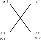
Figure 13: The matrix element $S_{a_{1}a_{2}}^{a^{\prime}_{1},a^{\prime}_{2}}$ corresponds to the process illustrated here.

Relativistic invariance contrains the S matrix to depend on the difference of rapidities $\alpha_{1}-\alpha_{2}$.

In the case of the sine-Gordon model, perturbation in $\beta$, considerations of (quantum affine) symmetry, minimality and consistency assumptions, lead to the following results. The spectrum is made up of the kink and antikink of mass $M\propto\Lambda^{1\over 2-2g}$, together with breathers. For $n-1<{1\over g}\leq n$, there are $n-2$ such breather states. Their masses are $M_{k}=2M\sin\left[k\pi g/2(1-g)\right]$.

The kink S-matrix is closely related to the matrix of Boltzmann weights in the 6-vertex model. There are three key amplitudes

$$a(\alpha) =\sin[\gamma(\pi+i\alpha)]Z(\alpha)$$

$$b(\alpha) =-\sin(i\gamma\alpha)Z(\alpha)$$

$$c(\alpha) =\sin(\gamma\pi)Z(\alpha),$$ (167)

where $\gamma={1\over g}-1$.

Figure 14: The three types of possible processes involving kink and antikink.

The element $a(\alpha_{1}-\alpha_{2})$ describes the process $\left|\alpha_{1}\alpha_{2}\right>_{++}\rightarrow\left|\alpha_{1}\alpha_{2}\right>_{++}$, as well as $\left|\alpha_{1}\alpha_{2}\right>_{--}\rightarrow\left|\alpha_{1}\alpha_{2}\right>_{--}$, $b$ describes $+-\to+-$, $c$ describes the non-diagonal process $+-\to-+$ (see figure 14), and there is a symmetry under interchange of kink to antikink (corresponding to $\Phi\to-\Phi$).

Exercise: Show that (167) gives rise, indeed, to a solution of the Yang Baxter equation. Hint: proceed graphically as sketched in figure 15 - to represent the matrix multiplications of YB, simply draw all the physical processes that connect a given pair of initial and final states, and add up their amplitudes.

Figure 15: The three types of possible processes involving kink and antikink.

The function $Z(\alpha)$ is a normalization factor, which can be written as

$$Z(\alpha)={-1\over\sin[\gamma(\pi+i\alpha)]}\exp\left(i\int_{-\infty}^{\infty}{dy\over 2y}\sin{2\alpha\gamma y\over\pi}{\sinh[(\gamma-1)y]\over\sinh y\cosh(\gamma y)}\right).$$

The breather-kink and breather-breather $S$ matrices are well known ; we do not write them down here (see below for some examples, and in the appendix).

These S matrices of course are not only characterized by the fact that they must solve the Yang-Baxter equation: there are several other physical requirements, like unitarity and crossing symmetry. In the formula above, these translate into the relations

$$a(\alpha)=b(i\pi-\alpha)$$

$$c(\alpha)=c(i\pi-\alpha)$$ (168)

form which unitarity $S(\alpha)S(-\alpha)$ follows.

In addition, one must have a “closed bootstrap”: for instance, breathers appear as poles in the kink antikink scattering, and their S matrix can be computed using this fact (for a review see [45], [46]).

When $1/g$ is an integer, the bulk scattering is diagonal ($c$ vanishes) and $a=\pm b$. Therefore, the only allowed processes are transmissions: particles go through one another without exchanging quantum numbers. This is the simplest case, to which we will restrict in what follows.

It is reasonable to think of the S matrix, together with the mass spectrum, as the quantum equivalent of the knowledge of the $\tau$ function in the classical case . We can then take the massless limit exactly as we did before, by letting the mass parameter $M\to 0$, and at the same time boosting the rapidities. One obtains then a collection of left and right moving kinks, antikinks and breathers. The LL and RR scattering matrices take exactly the same expressions as in the massive case in terms of the new rapidities $\theta$, while the LR S matrices go to constants, which can in most cases just be forgotten. This provides an alternative description of the free boson in terms of “massless scattering”. We will see in a little while how quantities of the conformal field theory can be recovered, if one wishes, within that description.

It is fair to stress here that the RR or LL scattering are hard to make sense of in the context of a true, physical scattering process. If particles have the label R say, this means they are moving at the speed of light in the right direction, so, for instance, all the lines in the figure 11 which illustrates the Yang Baxter equation become parallel! The point is that the scattering has to be interpreted in the massless limit as a set of commutation relations for creation operators, an idea which we will discuss below. The idea of massless scattering appeared a bit weird at the beginning [47], [50],[48], but its predictive power and favorable comparison with experiments gained it respectability quickly. A more rigorous approach along the lines of lattice regularizations is proposed in [49].

5.3 Back to the boundary sine-Gordon model

For the moment, we finish following the logic of the classical analysis in the quantum case. First, one can prove that the quantum sine-Gordon model with a bulk and boundary interaction

$$S={1\over 2}\int_{-\infty}^{0}dx\int dy\left[\left(\partial_{x}\Phi\right)^{2}+\left(\partial_{y}\Phi\right)^{2}+\Lambda\cos\beta\Phi(x,y)\right]+\lambda\int dy\cos{\beta\over 2}\Phi(0,y).$$ (169)

allows the existence of conserved quantities as well [51]. The proof proceeds in the same spirit as for the bulk case, and we are not going to reproduce it here, though it is an excellent exercise for the diligent reader.

Exercise: Show that, in the classical theory, the pair $T_{4},\Theta_{2}$ still leads to a conserved quantity provided there exists still another local quantiy $\theta_{3}$ such that

$$\left.T_{4}+\bar{\Theta}_{2}-\bar{T}_{4}-\Theta_{2}\right|_{x=0}={d\over dy}\theta_{3}$$ (170)

Show then, that for the sine-Gordon model with a potential $V[\Phi(x=0,y)]$ at the boundary, only the choice $V\propto\cos{1\over 2}(\Phi+\Phi_{0})$ allows the existence of the integral of motion.

Integrability means that the particles also have to scatter nicely at the boundary, ie scatter one by one, without particle production, in a way that is compatible with the bulk scattering. This latter condition can simply be expressed graphically as shown on figure 16, and corresponds to the “boundary Yang-Baxter” equation.

Figure 16: The boundary Yang-Baxter equation.

The problem of determining the reflection matrix is purely technical. It does have quite a simple answer in the massless limit. Introduce

$$R_{+-}(\theta)=R_{-+}(\theta)={-i\exp(\gamma\theta)\over 1-i\exp(\gamma\theta)}\exp\left[i\chi_{g}(\theta)\right]$$

$$R_{++}(\theta)=R_{--}(\theta)={1\over 1-i\exp(\gamma\theta)}\exp\left[i\chi_{g}(\theta)\right]$$

where $\chi_{g}$ is a phase that will disappear at the end of the computations, $\gamma={1\over g}-1$. The reflection matrix for coupling $\lambda$ is then given by $R(\theta-\theta_{B})$ where $T_{B}=e^{\theta_{B}}\propto\lambda^{1/(1-g)}$ (the exact correspondence depends on the regularization scheme; it is given in [36] in the case of dimensional regularization) is the equivalent of the Kondo temperature. As $\theta\to\infty$, $R_{++}\to 0$ (the scattering is completely off-diagonal) corresponding to Neumann boundary conditions, while as $\theta\to-\infty$, $R_{+-}\to 0$ (the scattering is completely diagonal) corresponding to Dirichlet boundary conditions. Notice also the unitarity condition $\left|R_{+-}\right|^{2}+\left|R_{++}\right|^{2}=1$.

6 The thermodynamic Bethe-ansatz: the gas of particles with “Yang-Baxter statistics”.

The thermodynamic Bethe ansatz was probably written first in [52] in the context of the XXZ model. Its use in quantum field theory, in particular to compute the central charge and study RG flows, was pioneered by a beautiful series of papers of Al. Zamolodchikov; see for instance [53]. A useful and pedagogical review on many of these topics can be found in [55].

6.1 Zamolodchikov Fateev algebra

It is convenient to think of the particles in terms of creation and annihilation operators. For this, let us introduce, still denoting the type of the particles by a label $a$, operators $Z_{a}(\theta)$ and $Z_{a}^{\dagger}(\theta)$ satisfying the relations

$$Z_{a_{1}}(\theta_{1})Z_{a_{2}}(\theta_{2}) = S_{a_{1}a_{2}}(\theta_{1}-\theta_{2})Z_{a_{2}}(\theta_{2})Z_{a_{1}}(\theta_{1})$$

$$Z^{\dagger}_{a_{1}}(\theta_{1})Z^{\dagger}_{a_{2}}(\theta_{2}) = S_{a_{1}a_{2}}(\theta_{1}-\theta_{2})Z^{\dagger}_{a_{2}}(\theta_{2})Z^{\dagger}_{a_{1}}(\theta_{1})$$

$$Z_{a_{1}}(\theta_{1})Z_{a_{2}}^{\dagger}(\theta_{2}) = S_{a_{1}a_{2}}(\theta_{1}-\theta_{2})Z^{\dagger}_{a_{2}}(\theta_{2})Z_{a_{1}}(\theta_{1})+2\pi\delta_{a_{1}a_{2}}\delta(\theta_{1}-\theta_{2})$$ (171)

Here, we restricted to the case of diagonal scattering. Note that the compatibility between the first two relations uses unitarity in the form $S^{\dagger}(\theta)=S^{-1}(\theta)=S(-\theta)$. The space of states is generated by the kets

$$\left|\theta_{1},\ldots,\theta_{n}\right>_{a_{1},\ldots,a_{n}}=Z_{a_{1}}^{\dagger}(\theta_{1})\ldots Z_{a_{n}}^{\dagger}(\theta_{n})\left|0\right>,$$ (172)

where $\left|0\right>$ denotes the physical vacuum. Similarly, the dual space is generated by the bras

$$\left<\theta_{n},\ldots,\theta_{1}\right|=\left<0\right|Z_{a_{n}}(\theta_{n})\ldots Z_{a_{1}}(\theta_{1})$$ (173)

The metric is, from (171), induced by

$${}_{a_{1}}\left<\theta_{1}|\theta_{2}\right>_{a_{2}}=2\pi\delta_{a_{1}a_{2}}\delta(\theta_{1}-\theta_{2})$$ (174)

If for instance $\theta_{1}>\theta_{2}$, then the in and out states are, respectively

$$\left|\theta_{1},\theta_{2}\right>_{a_{1}a_{2}}^{in}=\left|\theta_{1},\theta_{2}\right>_{a_{1}a_{2}}$$

$$\left|\theta_{1},\theta_{2}\right>_{a_{1}a_{2}}^{out}=\left|\theta_{2},\theta_{1}\right>_{a_{1}a_{2}}$$ (175)

When the rapidity sets are not ordered, one obtains states which are neither in nor out; or course they are related to either of these by products of S matrix elements.

To make things more concrete, let us discuss briefly wave functions in coordinate representation, restricting for simplicity to two particles. To satisfy the relations (171), it is easy to see that the wave function must have a singularity at coincident coordinates, and be of the form

$$\left|\theta_{1}\theta_{2}\right>_{a_{1}a_{2}}\propto\int_{x_{1}<x_{2}}dx_{1}dx_{2}\ e^{i(P_{1}x_{1}+P_{2}x_{2})}\left|x_{1},x_{2}\right>_{a_{1}a_{2}}-S_{a_{1}a_{2}}(\theta_{1}-\theta_{2})\int_{x_{1}>x_{2}}dx_{1}dx_{2}\ e^{i(P_{1}x_{1}+P_{2}x_{2})}\left|x_{1},x_{2}\right>_{a_{1}a_{2}}.$$ (176)

where we assumed that the particles are fermions, $S(0)=-1$. Equivalently, one has

$$\left|x_{1}x_{2}\right>_{a_{1}a_{2}}\propto\int_{\theta_{1}>\theta_{2}}d\theta_{1}d\theta_{2}\ \left[e^{i(P_{1}x_{1}+P_{2}x_{2})}+S_{a_{1}a_{2}}(\theta_{1}-\theta_{2})e^{i(P_{1}x_{2}+P_{2}x_{1})}\right]\left|\theta_{1},\theta_{2}\right>_{a_{1}a_{2}}^{in}$$ (177)

where we see the appearance of the well known Bethe wave function [55] .

6.2 The TBA

The next step is to get a handle on the massless scattering description. The latter turns out to be quite convenient to discuss thermodynamic properties, and this is what we shall start with.

As a simple example we consider a hypothetical theory made up of a single type of massless particle, say right-moving, with energy and momentum parametrized as in (152). The scattering is described by a single $S$-matrix element $S_{RR}$. Quantizing a gas of such particles on a circle of length $L$ requires the momentum of the $i$th particle to obey (we have set $\hbar=1$)

$$\exp\left(ime^{\theta_{i}}L\right)\prod_{j\neq i}S_{RR}(\theta_{i}-\theta_{j})=1.$$ (178)

One can think of this intuitively as bringing the particle around the world through the other particles; one obtains a product of two-particle $S$-matrix elements because the scattering is factorizable. A bit more rigorously, one can deduce this from the wave function as in (176)

Going to the $L\rightarrow\infty$ limit, we introduce the density of rapidities indeed occupied by particles $\rho(\theta)$ and the density of holes $\tilde{\rho}$. A hole is a state which is allowed by the quantization condition (178) but which is not occupied, so that the density of possible rapidities is $\rho(\theta)+\rho^{h}(\theta)$. Taking the derivative of the log of (178) yields

$$2\pi[\rho(\theta)+\rho^{h}(\theta)]=mLe^{\theta}+\int_{-\infty}^{\infty}K(\theta-\theta^{\prime})\rho(\theta^{\prime})d\theta^{\prime},$$ (179)

where

$$K(\theta)={1\over i}{d\over d\theta}\ln S(\theta).$$

To determine which fraction of the levels is occupied we do the thermodynamics, following the pioneering work of Yang and Yang. The energy is

$${\cal E}=\int_{-\infty}^{\infty}\rho(\theta)me^{\theta}d\theta,$$

and the entropy is

$${\cal S}=\int_{-\infty}^{\infty}\left[(\rho+\rho^{h})\ln(\rho+\rho^{h})-\rho\ln(\rho)-\rho^{h}\ln(\rho^{h})\right]d\theta.$$

Exercise: derive this relation by using Stirling’s formula $\Gamma(z)\approx z^{z-{1\over 2}}e^{-z}\sqrt{2\pi}$.

The free energy ${\cal F}=({\cal E}-T{\cal S})$ is found by minimizing it with respect to $\rho$. The variations of ${\cal E}$ and ${\cal S}$ are

$$\delta{\cal E}= \int_{-\infty}^{\infty}\delta\rho me^{\theta}d\theta$$

$$\delta{\cal S}= \int_{-\infty}^{\infty}\left[(\delta\rho+\delta\rho^{h})\ln(\rho+\rho^{h})-\delta\rho\ln(\rho)-\delta\rho^{h}\ln(\rho^{h})\right]d\theta$$

It is convenient to parametrize

$${\rho(\theta)\over\rho^{h}(\theta)}=\exp\left(-{\epsilon\over T}\right)$$ (180)

giving

$$\delta{\cal S}=\int_{-\infty}^{\infty}\left[\delta\rho\ln\left(1+e^{\epsilon/T}\right)+\delta\rho^{h}\ln\left(1+e^{-\epsilon/T}\right)\right]d\theta.$$

Using (179) allows us to find $\tilde{\rho}$ in terms of $\rho$. Denoting convolution by $\star$, this gives $2\pi(\delta\rho+\delta\rho^{h})=K\star\delta\rho$ so

$$\delta{\cal S}=\int_{-\infty}^{\infty}\left[{\epsilon\over T}+{K\over 2\pi}\star\ln\left(1+e^{-\epsilon/T}\right)\right]\delta\rho d\theta.$$

Hence the extremum of ${\cal F}$ occurs for

$$me^{\theta}=\epsilon+T{K\over 2\pi}\star\ln\left(1+e^{-\epsilon/T}\right).$$ (181)

and one has then, expressing $\rho^{h}$ from (179) and using (181)

$${\cal F}=-LT^{2}{m\over 2\pi T}\int_{-\infty}^{\infty}e^{\theta}\ln\left(1+e^{-\epsilon/T}\right)d\theta.$$ (182)

It is a simple exercise to show that this formula, together with (181), generalizes to a theory with several species of particles, provided the scattering is diagonal. This corresponds to the case ${\beta^{2}\over 8\pi}=g={1\over t}$, $t$ an integer, to which we restrict in what follows. In that case, recall that we have a kink and antikink of mass parameter $m$, and breathers of mass parameter $m_{k}=2m\sin{k\pi\over 2(t-1)}$, with $k=1,\ldots,t-2$. We will also allow for different chemical potentials $\mu_{k}$ for the various particles. Defining now $\epsilon$’s through

$${\rho_{j}(\theta)\over\rho^{h}_{j}(\theta)}=\exp\left({\mu_{j}-\epsilon_{j}\over T}\right)$$ (183)

the equivalent of (179) is now

$$2\pi[\rho_{j}(\theta)+\rho^{h}_{j}(\theta)]=m_{j}Le^{\theta}+\sum_{k}\int_{-\infty}^{\infty}K_{jk}(\theta-\theta^{\prime})\rho_{k}(\theta^{\prime})d\theta^{\prime},$$ (184)

and the equivalent of (181)

$$m_{j}e^{\theta}=\epsilon_{j}+T\sum_{k}{K_{jk}\over 2\pi}\star\ln\left(1+e^{\mu_{k}-\epsilon_{k}\over T}\right).$$ (185)

The equivalent of (182) is, in turn:

$${\cal G}={\cal E}-T{\cal S}-\sum_{k}\mu_{k}{\cal N}_{k}=-LT^{2}\sum_{k}{m_{k}\over 2\pi T}\int_{-\infty}^{\infty}e^{\theta}\ln\left(1+e^{\mu_{j}-\epsilon_{k}\over T}\right)d\theta.$$ (186)

For the case $g={1\over 3}$ for instance, one has

$$K_{bb}=2K_{++}=2K_{+-}=-{2\over\cosh\theta}$$

$$K_{b+}=K_{+b}=-2\sqrt{2}{\cosh\theta\over\cosh 2\theta}$$ (187)

It has become common in the literature to reformulate the TBA in a convenient form by using simple diagrams. It is a laborious but straightforward exercise to demonstrate, using the kernels given in the appendix, that (185) is equivalent to the following simple system

$$\epsilon_{j}=T\sum_{k}N_{jk}{s\over 2\pi}\star\ln\left(1+e^{\epsilon_{k}-\mu_{k}\over T}\right)$$ (188)

Here, $s(\theta)={(t-1)\over\cosh(t-1)}(\theta)$, $N_{jk}=1$ if the nodes $j$ and $k$ are neighbours on the following diagram, $0$ otherwise

$\hskip 156.49014pt\bigcirc\hskip 7.11317pt+$ $\hskip 153.6447pt\bigcirc\hskip 8.5359pt-$ $\hskip 145.10922pt\Big{/}$ $\hskip 142.26378pt\Big{\backslash}$ $1\hskip 28.45274pt2\hskip 36.98866pts\hskip 22.76228ptt-3$ $\bigcirc$——$\bigcirc$– – – –$\bigcirc$– – –$\bigcirc$——$\bigcirc$     $t-2$

Exercise: establish this for the case $g={1\over 3}$.

The equations (188) have to be supplemented by the boundary conditions

$$\epsilon_{j}\approx m_{j}e^{\theta},\ \theta>>1$$ (189)

6.3 A standard computation: the central charge

The thermodynamics of a chiral theory like the one we just studied is not so exciting; this is because, after all, the $1+1$ theory is conformal invariant, so the results at different temperatures are essentially equivalent. This can easily be seen on the TBA equations: a change in $T$, or the mass scale $m$, can be fully absorbed by a boost of the particles, ie a shift of rapidities, exactly like for the changes in mass scale encountered before. As a result, we see that the integrals in (182) are independent of the temperature, so ${\cal F}\propto LT^{2}$.

That this is so, and the coefficent of proportionality, are directly related with considerations from the beginning of these lectures. Indeed, we have ${\cal F}=-T\ln Z$, where $Z$ is the partition function of the one dimensional quantum field theory at temperature $T$. In Euclidean formalism, this corresponds to a theory on a torus with finite size in time direction $R=1/T$. By modular invariance, identical results should be obtained if one quantizes the theory with $R$ as the space coordinate . For large $L$, $Z=e^{-E(R)L}$, where $E(R)$ is the ground-state (Casimir) energy with space a circle of length $R$. Thus ${\cal F}=LE(R)/R$. Conformal invariance requires that at a fixed point this Casimir energy is $E(R)=-{\pi c\over 6R}$, where $c$ is the central charge. Going back to the thermal point of view, ${\cal F}=-{L\pi cT^{2}\over 6}$ and the specific heat is ${\cal C}={L\pi cT\over 3}$.

It is possible to analytically find this central charge from (181). This is a bit technical, but worth studying, since it is a crucial a posteriori test of the whole thing. We take the derivative of (181) with respect to $\theta$ and solve for $e^{\theta}$. Substituting this in (182), we have

$${\cal F} =-{TL\over 2\pi}\int d\theta\left[{d\epsilon\over d\theta}\ln(1+e^{-\epsilon/T})-\int{d\theta^{\prime}\over 2\pi}\ln(1+e^{-\epsilon(\theta)/T})K(\theta-\theta^{\prime}){d\epsilon\over d\theta^{\prime}}{1\over 1+e^{\epsilon(\theta^{\prime})/T}}\right]$$ (190)

$$=-{TL\over 2\pi}\int d\theta{d\epsilon\over d\theta}\left[\ln(1+e^{-\epsilon/T})+{\epsilon-me^{\theta}\over T}{1\over 1+e^{\epsilon(\theta)/T}}\right]$$

$$=-{\cal F}-{TL\over 2\pi}\int d\theta{d\epsilon\over d\theta}\left[\ln(1+e^{-\epsilon/T})+{\epsilon/T\over 1+e^{\epsilon/T}}\right],$$

where we use (181) again to get to the second line. We can replace the integral over $\theta$ with one over $\epsilon$, giving an ordinary integral

$${\cal F}=-{TL\over 4\pi}\int_{\epsilon(-\infty)}^{\infty}d\epsilon\left[\ln(1+e^{-\epsilon/T})+{\epsilon/T\over 1+e^{\epsilon(\theta)/T}}\right],$$

A change of variables gives

$${\cal F}=-{T^{2}L\over 2\pi}{\cal L}\left({1\over 1+x_{0}}\right),$$ (191)

where ${\cal L}(x)$ is the Rogers dilogarithm function

$${\cal L}(x)=-{1\over 2}\int_{0}^{x}\left({\ln(1-y)\over y}+{\ln y\over 1-y}\right)dy,$$

and $x_{0}\equiv\exp[\epsilon(-\infty)/T]$ is obtained from (181) as

$${1\over x_{0}}=\left(1+{1\over x_{0}}\right)^{I},$$ (192)

with $I={1\over 2\pi}\int K$.

For example, when the $S$ matrix is a constant, $K=0$, $x_{0}=1$ and

$${\cal F}=-{LT^{2}\pi\over 24},$$ (193)

where we used $L(1/2)={\pi^{2}\over 12}$. Here we find $c_{L}={1\over 4}$. In a left-right-symmetric quantum field theory, the right sector makes the same contribution, giving the total central charge $c={1\over 2}$ required for free fermions.

Similar computations can be carried out for more complicated theories, leading to beautiful expressions of central charges in terms of sums of dilogarithms (see eg [56]). In the case of interest, one finds of course $c=1$.

6.4 Thermodynamics of the flow between N and D fixed points

We now wish to do the thermodynamics in the presence of the boundary, to obtain the boundary free energy, and the associated flow of boundary entropies. To start, it is better to map the problem onto a line of length $2L$ ($-L<x<L$) by considering the left movers to be right movers with $x>0$. Thus we have only R movers scattering among themselves and off the boundary, which can now be thought of as an impurity (a particle with rapidity $\theta_{B}$). The reflection matrix becomes a transmission matrix, with appropriate relabellings, for instance $R_{+-}\to T_{++}$, etc. (This trick is the same than what we did for boundary conformal field theory, and can only be used in the massless limit.). For simplicity, we put periodic boundary conditions on the system; these do not change the boundary effects at $x=0$.

Recall we consider only the case $\gamma={1\over g}-1$ a positive integer, where the bulk scattering is diagonal. The impurity scattering still is not, but we can redefine our states to be $\left|1,2\right>\equiv(\left|+\right>\pm\left|-\right>)/\sqrt{2}$ so that the impurity scattering is now diagonal:

$$T_{11}(\theta)=R_{++}+R_{+-} =\exp\left[i\chi_{g}(\theta)\right]$$

$$T_{22}(\theta)=R_{++}-R_{+-} =\tanh\left({\gamma\theta\over 2}-{i\pi\over 4}\right)\exp\left[i\chi_{g}(\theta)\right].$$ (194)

We can now write the Bethe equations. These differ from the bulk ones only by the presence of the additional impurity scattering

$$2\pi(\rho_{j}(\theta)+\rho_{j}^{h}(\theta))=m_{j}e^{\theta}+\sum_{k}K_{jk}\star\rho_{k}(\theta)+{1\over 2L}\kappa_{j}(\theta-\theta_{B})$$ (195)

where

$$K_{jk}(\theta) = {1\over i}{d\over d\theta}\ln S_{jk}(\theta)$$

$$\kappa_{j}(\theta-\theta_{B}) = {1\over i}{d\over d\theta}\ln R_{j}(\theta-\theta_{B}).$$ (196)

The effect of the boundary is seen in the last piece of (195) proportional to $1/L$.

The minimization equations are independent of the boundary terms, since these do not appear directly in ${\cal E}$ or ${\cal S}$, and they disappear when one takes a variation of (195). Thus equations (185) still hold.

Boundary terms do enter the free energy or the grand potential however when one rewrites it in terms of the $\epsilon$’s. One finds

$${\cal F}={\cal F}_{bulk}-T\int{d\theta\over 2\pi}\sum_{j=1}^{t}\kappa_{j}(\theta-\ln(T/T_{B}))\ln(1+e^{-\epsilon_{j}(\theta)}).$$ (197)

As discussed before, ${\cal F}_{bulk}=-{\pi c\over 6}T^{2}L$ in a massless bulk theory, where $c$ is the central charge of the conformal field theory, $c=1$ here. The second term in (197) is the boundary free energy.

Although the equations (185) for $\epsilon(\theta)$ cannot be solved explicitly for all temperatures, the free energy is easy to evaluate as $T\to 0$ and $T\to\infty$, as we will show next. Moreover, one can extract the analytic values of critical exponents by looking at the form of the expansions around these fixed points. Also, they are straightforward to solve numerically for any $T$.

Several notes of caution are necessary. At the order we are working, the formula for the entropy is not quite correct, because there are $1/L$ corrections to the Stirling formula used in its derivation. Also, at this order, the logarithm of the partition function is not ${\cal E}-T{\cal S}$: it depends not only on the saddle point value of the sum over all states, but also on fluctuations. Their net effect is that we cannot compute the $g$ factors from ${\cal F}$ alone. However, both of these corrections are subleading contributions to the bulk free energy, and do not depend on the boundary conditions. Therefore we can still compute differences of $g$ factors from ${\cal F}$; the corrections are independent of the boundary scale $\theta_{B}$ and cancel out of the difference.

We can evaluate the impurity free energy explicitly in several limits. In the IR limit $T/T_{B}\rightarrow 0$ the integral is dominated by $\theta\rightarrow\infty$ where the source terms in (185) become very big. Hence $\epsilon_{r}(\infty)=\infty$ and the impurity free energy vanishes in this limit. In the UV limit $T/T_{B}\rightarrow\infty$ the integrals are dominated by the region where $-\theta$ is large so that the source terms disappear in (185) and the $\epsilon_{r}$ go to constants. These are found by using the alternative form (188), which reads here, denoting $x_{j}=e^{\epsilon_{j}/T}$

$$x_{j}=\prod_{k}(1+x_{k})^{N_{jk}/2}$$ (198)

One finds

$$x_{n}\equiv e^{\epsilon_{n}(-\infty)/T}=(n+1)^{2}-1;\qquad\quad x_{1,2}=\gamma$$ (199)

Therefore we obtain

$$\ln{g_{N}\over g_{D}}= \left.{-{\cal F}_{imp}\over T}\right|_{UV}-\left.{-{\cal F}_{imp}\over T}\right|_{IR}$$

$$= \sum_{n=1}^{t-2}I^{(n)}\ln(1+1/x_{n})+(I^{(+)}+I^{(-)})\ln(1+1/x_{\pm})$$ (200)

where

$$I^{(r)}\equiv\int{d\theta\over 2\pi}\kappa_{r}(\theta)=\tilde{\kappa}(0).$$

From results given in the appendix, one finds $I^{(n)}=n/2$ and $I^{(+)}+I^{(-)}=\gamma/2$, and thus

$$\ln{g_{N}\over g_{D}} = {\gamma\over 2}\ln{\gamma+1\over\gamma}+\sum_{n=1}^{\gamma-1}{n\over 2}\ln{(n+1)^{2}\over n(n+2)}$$ (201)

$$= {1\over 2}\ln(\gamma+1)={1\over 2}\ln t.$$

This is in agreement with the ratio calculated from conformal field theory.

We can also find the dimension of the perturbing operators. From the equations one deduces the following expansions for $T/T_{B}$ large:

$$Y_{r}(\theta)=e^{\epsilon_{r}(\theta)}=\sum_{j}Y_{r}^{(j)}e^{-2j\gamma\theta/(\gamma+1)}.$$

As a result it is straightforward to see that near $\lambda=0$, ${\cal F}$ can be expanded in powers of $(T_{B}/T)^{2\gamma/(\gamma+1)}$. On the other hand we expect ${\cal F}$ to be an analytic function of $\lambda^{2}$. Hence

$$\lambda\propto\left(me^{\theta_{B}}\right)^{\gamma/(\gamma+1)}.$$ (202)

This agrees with the conformal result that the perturbing operator $\cos[\beta\Phi(0)/2]$ has boundary dimension $d=1/(\gamma+1)=\beta^{2}/8\pi$. In the IR limit of $T/T_{B}$ small, one can expand out the kernels $\kappa_{r}$ in powers of $\exp(\theta_{b}-\theta)$. This leads to the fact that the irrelevant operator which perturbs the Dirichlet boundary conditions has dimension $d$=2. This is the energy-momentum tensor. (Recall that there is another irrelevant operator in the spectrum with dimension $d=\gamma+1$, which for $0\leq\gamma<1$ is the appropriate perturbing operator.)

7 Using the TBA to compute static transport properties

Let us pause for a moment to compare the gas of Yang-Baxter interacting quasi particles to say free fermions. Within the TBA, the interactions have been fully encoded into non trivial pseudo energies $\epsilon_{j}(\theta)$: that is, at temperature $T$, the filling fractions of the various species are not independent, but correlated via the coupled integral equations discussed previously. This has some striking consequences. For instance, we see from (199) that the filling fraction of kinks or antikinks at rapidity $-\infty$ (ie at vanishing bare energy) is $f={1\over t}$. Except for $t=2$ (which is a free fermion theory) there is no symmetry between particles and holes. It is important to realize that the interactions would have other effects, in general, for other questions asked. For instance, in the case of free fermions, the total density $n=\rho+\rho^{h}$, $\rho=nf$, the fluctuations also depend on the $\epsilon_{j}$ through the well known formula $\overline{\left(\Delta\rho\right)^{2}}=nf(1-f)$. Such a formula does not hold in the present case: the fluctuations of the various species are correlated - their computation plays an important role in the DC noise at non vanishing temperature and voltage, see [57]. Similarly, physical operators have complicated matrix elements in the multiparticle basis; the current for instance is able to create any neutral configuration of quasiparticles by acting on the vacuum. There is thus a somewhat deceptive simplicity in what we have done so far. However, for the DC conductance, it turns out that the knowledge of the distribution functions is all that is necessary, so for that particular aspect, our quasiparticles are not so far from free ones.

7.1 Tunneling in the FQHE

At this stage, it is useful to recall the tunneling problem of the introduction: we had L and R moving electrons that were backscattered by the impurity. Certainly if a R moving particle bounces back on the gate voltage to become a left one, the charge $Q_{R}+Q_{L}$ is conserved. Now $Q_{L}+Q_{R}$ is essentially the charge of the even field in the manipulations discussed in the introduction, which we found has no dynamic indeed. Now when a R mover bounces back as a L mover, there is a change in the non conserved charge $Q\equiv Q_{R}-Q_{L}$; this one is proportional to the charge of the odd field, which has a non trivial dynamics. Now, following carefully the formulas for bosonization, one finds the simple result that a right moving kink, for which ${\beta\over 2\pi}\int\partial_{x}\Phi=1$, also has physical charge $Q=1$, and similarly for antikinks and left moving particles. Therefore, the non conservation of the physical charge due to backscattering is the same as the non conservation of charge in the boundary sine-Gordon model. More precisely, when a kink comes in and bounces back as an antikink, as happens most of the time near the UV fixed point (Neumann boundary conditions), the charge $Q$ is conserved in the original problem. On the other hand, when a kink bounces back as a kink, as happens near the IR fixed point (Dirichlet boundary conditions), the charge in the original problem is not conserved; rather, $\Delta Q=-2$. Let me stress here that the kink in the boundary sine-Gordon theory however would look horribly complicated in the original problem, because the changes of variables we have performed are non local. Only the conserved charge is easy to follow .

7.2 Conductance without impurity

In the absence of impurity, that is with Neumann boundary conditions in the original boundary problem, charge is straightforwardly transported. A right moving kink or antikink just goes through. Of course, if there are as many particles of each specie, no current is transported overall. If however, a voltage $V$ is applied, kink and antikink are at a different chemical potential, $\mu=\pm{V\over 2}$ - this follows since the $U(1)$ charge in the boundary sine-Gordon model is nothing but the physical charge $Q$. The current that flows through the system is thus

$$I=\int_{-\infty}^{\infty}(\rho_{+}-\rho_{-})(\theta)d\theta$$ (203)

We can use our TBA to evaluate this expression quickly. First, we introduce the filling fractions

$$f_{\pm}={1\over 1+e^{(\epsilon_{\pm}\mp{V\over 2})/T}}$$ (204)

Second, we observe that the very convenient identity $n_{j}=\rho_{j}+\rho_{j}^{h}={1\over 2\pi}{d\epsilon_{j}\over d\theta}$ holds, and that, moreover, $\epsilon_{+}=\epsilon_{-}\equiv\epsilon$.

Exercise: Prove these two statements by staring at the TBA equations.

It thus follows that

$$I={1\over 2\pi}\int_{-\infty}^{\infty}\left(f_{+}-f_{-}\right){d\epsilon\over d\theta}d\theta$$ (205)

and thus

$$I={T\over 2\pi}\int_{-\infty}^{\infty}d\theta{d\over d\theta}\ln\left[{1+e^{-V/2T}e^{-\epsilon/T}\over 1+e^{V/2T}e^{-\epsilon/T}}\right]$$ (206)

The current is thus entirely determined by the values of $\epsilon$ at $\pm\infty$, exactly like for the central charge. As before, $\epsilon(\infty)=\infty$, but the value of $\epsilon(-\infty)$ now does depend on the voltage. One finds in fact, solving again (188) but with a voltage,

$$e^{\epsilon_{n}(-\infty)/T}=\left[{\sinh(n+1)V/2tT\over\sinh V/2tT}\right]^{2}-1,~{}~{}e^{\epsilon_{\pm}(-\infty)/T}={\sinh(t-1)V/2tT\over\sinh V/2tT}$$ (207)

(observe one recovers the result (199) as $V\to 0$) from which an elementary computation shows the simple result (recall $g={1\over t}$)

$$I={gV\over 2\pi}$$ (208)

The bizarre factor of $2\pi$ occurs here because we have set $e=\hbar=1$ (recall that in physical units, $I=g{e^{2}\over h}V$).

Exercise: Prove the last two formulas.

This is what one expected, and of course there are quicker ways to derive this result. The point however, is that the same computation carries over without much additional difficulty to the case where the impurity is present.

7.3 Conductance with impurity

In the general case, we will write the source drain current as $I=I_{0}+I_{B}$ where $I_{0}={gV\over 2\pi}$ is the current in the absence of backscattering, and $I_{B}$ is the backscattered current. In the original problem, $I_{B}$ is for instance the rate at which the charge of the right moving edge is depleted. Of course, $\partial_{t}Q_{L}=-\partial_{t}Q_{R}$ in each hopping event, so $I_{B}=\partial_{t}{Q\over 2}$. In the steady state this rate is constant. When for instance $V$ is positive, there are more kinks than antikinks injected with a thermal distribution into the system from their respective infinite reservoirs; it is assumed that these reservoirs are so big that the backscattering does not change their properties.

We now derive an analytic expression for this backscattering current using a kinetic rate equation for quasiparticles of the Bethe ansatz. It is possible to compute the rate of change of $\Delta Q/2$ in the basis of the Bethe ansatz quasiparticles, since each scattering event of a kink (antikink) into an antikink (kink) changes the physical charge $\Delta Q/2$ by $-1$ (by $(+1)$). This kinetic equation is of course very familiar. However, in general there would be no reason why it should be applicable to an interacting system. But it is exact in the case that we are considering, even though the system is interacting. The reason for this lies in the constraints of integrability: as discussed above, in the very special quasiparticle basis of the Bethe ansatz, these quasiparticles scatter off of the point contact independently (“one-by-one”), and all quasiparticle production processes are absent .

This allows us to express the rate of change in $\Delta Q$, in terms of the transition probability $|T_{+-}|^{2}$ (recall that in the unfolded point of view $T_{+-}=R_{++}$) and the number of kinks and antikinks (carriers of charge $\Delta Q=\pm 1$) in the rapidity range between $\theta$ and $\theta+d\theta$

$$n_{\pm}(\theta)f_{\pm}(\theta)d\theta,$$

where $n_{\pm}$ is the density of states and $f_{\pm}$ are the filling fractions. The number of kinks of rapidity $\theta$ that scatter into antikinks per unit time is

$$|T_{+-}(\theta)|^{2}\rho_{+-}d\theta$$ (209)

where $\rho_{+-}$ is the probability that the initial kink state is filled and the final antikink state is empty (in all these quantities, there is also a $V$ dependence, which we keep implicit here). For a system of free fermions we would have

$$\rho_{+-}=f_{+}(1-f_{-})$$

but in our interacting system we only have

$$\rho_{+-}=f_{+}-f_{+-}$$

where $f_{+-}$ is the probability that both, the kink and the antikink states are filled. For the number of antikinks of rapidity $\theta$ that scatter into kinks per unit time one finds a formula similar to (209), with $\rho_{+-}\to\rho_{-+}$. In the final rate equation, only the difference between these two probabilities

$$\rho_{+-}-\rho_{-+}=f_{+}-f_{-}$$

appears. Notice that the unknown $f_{+-}=f_{-+}$ has cancelled out (it can in fact be determined by techniques more elaborate than the TBA [57]). Therefore, the backscattering current is

$$I_{B}(V)=-\int d\theta~{}n(\theta)|T_{+-}(\theta-\theta_{B})|^{2}[f_{+}(\theta)-f_{-}(\theta)]$$ (210)

All ingredients in this formula are exactly known: the scattering matrix has a simple analytic form and the occupation factors and densities of state are obtained exactly from the thermodynamic Bethe ansatz (TBA). Notice that this equation is valid for any value of the driving voltage $V$. It thus automatically describes non-equilibrium transport.

By the same manipulations as before, it then follows that

$$I={1\over 2\pi}\int_{-\infty}^{\infty}\left(f_{+}-f_{-}\right)\left|T_{++}\right|^{2}{d\epsilon\over d\theta}d\theta={T\over 2\pi}\int_{-\infty}^{\infty}d\theta{1\over e^{2(t-1)(\theta-\theta_{B})}}{d\over d\theta}\ln\left[{1+e^{-V/2T}e^{-\epsilon/T}\over 1+e^{V/2T}e^{-\epsilon/T}}\right]$$ (211)

Of special interest is the linear conductance, which we obtain by taking a derivative at $V=0$; this gives, after reinserting the factor $2\pi$,

$$G={(t-1)\over 2}\int_{-\infty}^{\infty}d\theta{1\over 1+e^{\epsilon/T}}{1\over\cosh^{2}\left[(t-1)(\theta-\ln(T_{B}/T))\right]}$$ (212)

The resulting curve is shown in figure 17, together with experimental results [13] and the results of Monte Carlo simulations [14], for $g={1\over 3}$.

Figure 17: Comparison of the field theoretic result with MC simulations and experimental data for $g={1\over 3}$.

The agreement with the simulations is clearly very good (the is one and only one fitting parameter - the horizontal scale - , accounting for the unknown, non universal ratio of the experimental gate voltage (a “bare” quantity) to the parameter $\lambda$ in our renormalized field theory). As far as the experimental data go, it is also very satisfactory, except in the strong backscattering regime. Recall however that the field theoretic prediction holds true only in the scaling limit: the experimental data are still quite scattered for low values of $G$, indicating that this limit is not reached yet - actually the “noise” is of the same order of magnitude as the discrepancy from the theoretical curve, as reasonably expected.

Exercise: The problem had been solved previously [10] in the simplest case of $g={1\over 2}$, where one can refermionize the hamiltonian for the boson $\phi^{e}$. Look at this solution, and compare with what we have just done: what is the meaning of kink and antikink, what is the bulk scattering, the boundary scattering?

Conclusions: further reading and open problems

I am now leaving you at the beginning of a very exciting domain. Let me suggest some further reading and open problems.

These lectures have stopped short of really tackling the problem of boundary fixed points classification. Equipped with what you learned here, you should not have much difficulty reading the paper of J. Cardy on boundary states [32]. This paves the way to questions that are still open. For instance, the problem we have studied at length generalizes, for tunneling in quantum wires where the spin of the electrons has to be taken into account, to a “double sine-Gordon problem”, involving two bosons. Surprisingly it has been shown [10] that new non trivial fixed points do exist in that case, besides the obvious Neumann and Dirichlet possibilities. With a few exceptions [64], [65], nobody knows how these fixed points precisely look like! As I will mention again below, what we have discussed is also very close to the Kondo problem. You can learn more about fixed points and conformal invariance by reading the papers of Affleck and Ludwig on the multichannel Kondo problem [16]. There, you will also discover an aspect that I have neglected by lack of space: how multipoint correlators can be evaluated at fixed points by further using conformal invariance [18].

The integrable approach can also be pushed further to allow the computation of AC properties, together with space and time dependent Green functions, in the cross-over regime. The idea here still relies on massless scattering; but now, one has to evaluate matrix elements of physical operators, and these are usually pretty complicated. Moreover, an infinity of these matrix elements are a priori needed: for instance, the current operator is able to create any neutral configurations of quasiparticles out of the vacuum! It turns out however that, first, the matrix elements can be determined by algebraic techniques [59], [60] (the latter reference is recomended as a first reading; the first is a bit hard to read), and second, in many cases, only a few of these matrix elements are required to obtain controlled accuracy all the way from the UV to the IR fixed point. Using that technique, for instance the current current correlator itself can be evaluated, at least at $T=V=0$ [61] (there does remain a non trivial dependence upon space, time, and the coupling $\lambda$). Determining correlators with a finite temperature or voltage is still more difficult; some progress in that direction has been made [62], [63], but a lot remains to be done.

In another direction, for those of you who are more formally oriented, it should be clear that what I just described is the tip of an iceberg of beautiful mathematical structures: see [36],[66] and the series [67]. Let me just mention here that the Kondo problem, which would be described by

$$H\equiv H^{e}=\frac{1}{2}\int_{-\infty}^{0}dx\ \left[\Pi^{2}+(\partial_{x}\Phi)^{2}\right]+\lambda\left(S^{+}e^{-i\beta\Phi(0)/2}+S^{-}e^{i\beta\Phi(0)/2}\right),$$ (213)

is just around the corner: it actually does have deep relations with the boundary sine-Gordon model, and with the subject of quantum monodromy operators. Especially exciting results have actually appeared recently, concerning an exact duality between the UV and IR regimes of the problem [68],[69], and exhibiting tantalizing relations with the recent breakthroughs in 4D SUSY gauge theories [70].

It is also fair to stress that the methods developed within the context of quantum impurity problems can be generalized to different systems of physical interest in $1+1$ dimensions: an example is the amazing recent mapping of the two-ladder problem onto an $SO(8)$ Gross Neveu model [71]. It is very likely indeed that more such problems are awaiting us in the near future.

Finally, the traditional question is, can any of this be generalized to more than $1+1$? Well, the recent excitments in string theory are centered around somewhat similar ideas in $3+1$, where, roughly, integrability is replaced by supersymmetry, an incredibly powerful tool. As for $2+1$, I don’t quite think it’s over yet.

Acknowledgments: The material in these notes is partly based on collaborations with I. Affleck, P. Fendley, A. Leclair, F. Lesage, A. Ludwig, M. Oshikawa, P. Simonetti, S. Skorik and N. Warner; I also greatly benefitted from questions by the school students, the organizers, and my fellows co-lecturers - many thanks to all of them. The work was supported by the USC, the DOE, the NSF (through the NYI program), and the David and Lucile Packard Foundation.

Dedication: Many friends from “Le plateau” have disappeared since I left France, and their memory weighs very much on my mind. I am especially thinking of Heinz Schulz in this early december: it is to him that I would like to dedicate these notes.

Appendix: Kernels

We use the following convention for Fourier transform:

$$\tilde{f}(y)=\int^{\infty}_{-\infty}{d\theta\over 2\pi}e^{i2\gamma\theta y/\pi}f(\theta),$$

where $\gamma=t-1$. The bulk kernels $K_{jk}$ are well known; they can be written in the form ($\pm$ stand for kink and antikink)

$$\tilde{K}_{jk} = \delta_{jk}-2{\cosh y\cosh(\gamma-j)y\sinh ky\over\cosh\gamma y\sinh y}\qquad j,k=1\dots\gamma-1;\ j\geq k$$

$$\tilde{K}_{j,\pm} = -{\cosh y\sinh jy\over\cosh\gamma y\sinh y}$$

$$\tilde{K}_{\pm,\pm} = \tilde{K}_{\pm,\mp}=-{\sinh(\gamma-1)y\over 2\cosh\gamma y\sinh y}$$ (214)

with $K_{jk}=K_{kj}$. The boundary kernels are

$$\tilde{\kappa}_{j} = {\sinh jy\over 2\sinh y\cosh\gamma y}$$

$$\tilde{\kappa}_{-} = {\sinh(\gamma-1)y\over 2\sinh 2y\cosh\gamma y}+{1\over 2\cosh y}$$

$$\tilde{\kappa}_{+} = {\sinh(\gamma-1)y\over 2\sinh 2y\cosh\gamma y}.$$ (216)

Finally, $\tilde{s}={1\over 2\cosh y}$.

References

- [1] A.C. Hewson, The Kondo Problem to Heavy Fermions, Cambridge University Press, 1997
- [2] L. Saminadayar, D.C. Glattli, Y. Jin, B. Etienne, cond-mat/9706307, Phys. Rev. Lett. 75 (1997) 2526.
- [3] R. de-Picciotto, M. Reznikov, M. Heiblum, V. Umansky, G. Bunin, D. Mahalu, Nature 389 (1997) 162.
- [4] Perspectives in Quantum Hall Effects, S. Das Sarma and A. Pinczuk Eds., Wiley, 1997
- [5] A. J. Leggett, S. Chakravary, A.T. Dorsey, M. P. A. Fisher, A. Garg, and W. Zwerger, Rev. Mod. Phys. 59 (1987) 1.
- [6] U. Weiss, Dissipative Quantum Mechanics, World Scientifc, Singapore, 1998
- [7] N. Andrei, K. Furuya, J. Lowenstein, Rev. Mod. Phys. 55 (1983) 331.
- [8] P. B. Wiegmann, A. M. Tsvelick, JETP Lett. 38 (1983) 591
- [9] R Shankar, Rev Mod Phys 66 (1994) 129.
- [10] C L Kane and M P A Fisher, Phys. Rev. B46 (1992) 15233; B46 (1992) 7268.
- [11] F.D.M. Haldane, J. Phys. C14 (1981) 2585.
- [12] X.G. Wen, Phys. Rev. B41 (1990) 12838; Phys. Rev. B43 (1991) 11025.
- [13] F.P. Milliken, C.P. Umbach, R.A. Webb, Solid State Comm. 97, (1996) 309.
- [14] K. Moon, H. Yi, C.L. Kane, S.M. Girvin and M.P.A. Fisher, Phys. Rev. Lett. 71 (1993) 4381.
- [15] P Nozières, J. Low Temp. Phys. 17 (1974) 31; P Nozières and A Blandin, J de Physique (Paris) 41 (1980) 193.
- [16] For reviews, see I. Affleck, in Correlation Effects in Low-Dimensional Electron Systems; Eds.: A. Okiji and N. Kawakami (Springer-Verlag, Berlin, 1994), cond-mat/9311054; A. W. W. Ludwig, Int. J. Mod. Phys. B 8 (1994) 347; in Proceedings of the ICTP Summer School on Low Dimensional Quantum Field Theories for Condensed Matter Physicists, Trieste (Italy), Sept. 1992 Editors: S. Lundqvist, G. Morandi and Yu Lu (World Scientific, New Jersey, 1995); Physica B 199&200 (1994) 406 (Proceedings of the International Conference on Strongly Correlated Electron Systems, San Diego, 1993).
- [17] I. Affleck and A. W. W. Ludwig, Nucl. Phys. B 352 (1991) 849; ibid B 360 (1991) 641.
- [18] A. W. W. Ludwig and I. Affleck, Nucl. Phys. B 428 (1994) 545.
- [19] Les Houches, session XLIX, 1988, Fields, Strings and Critical Phenomena, Eds. E. Breźin and J. Zinn-Justin, Elsevier, New York, 1989.
- [20] J. L. Cardy, Conformal Invariance, in Phase Transitions, Eds. C. Domb and J. L. Lebowitz, vol. 11, Academic Press, New York, 1987.
- [21] J. Polchinski, in Proceedings of the 1994 Les Houches Summer School, hep-th/9411028.
- [22] P. Di Francesco, P. Mathieu, D. Seńećhal, Conformal Field Theory, Springer, New York, 1997.
- [23] A. M. Tsvelik, Quantum Field Theory in Condensed Matter Physics, Cambridge University Press, Cambridge, 1995.
- [24] P.Kadanoff and H.Ceva, Phys. Rev. B11 (1971) 3918.
- [25] M. Stone, Bosonization, World Scientific, Singapore, 1994.
- [26] M. Green, J. Schwarz and E. Witten, Superstring Theory, Cambridge University Press, 1987.
- [27] E. T. Whittaker, G. N. Watson, A Course of Modern Analysis, Cambridge University Press, 1990.
- [28] J. L. Cardy, Nucl. Phys. B240 (1984) 512.
- [29] T. Apostol, Modular Functions and Dirichlet Series in Number Theory, Springer (New York) 1990.
- [30] N. Ishibashi, Mod. Phys. Lett. A4 (1989) 251.
- [31] I. Affleck and M. Oshikawa, Nucl. Phys. B495 (1997) 533.
- [32] J. Cardy, Nucl. Phys. B324 (1989) 581.
- [33] I. Affleck and A. W. W. Ludwig, Phys. Rev. Lett. 67 (1991) 161.
- [34] P. Fendley, Phys. Rev. Lett. 71, (1993) 2485.
- [35] A B Zamolodchikov, JETP Lett 43 (1986) 730.
- [36] P. Fendley, F. Lesage and H. Saleur, J. Stat. Phys. 79 (1995) 799, hep-th/9409176.
- [37] I.G. Macdonald, Symmetric Functions and Hall Polynomials, Clarendon Press (1979); R.P. Stanley, Adv. in Math. 77 (1989) 76.
- [38] A. Schmid, Phys. Rev. Lett. 51 (1983) 1506.
- [39] P Fendley, A W W Ludwig, H Saleur, Phys. Rev. Lett. 74 (1995) 3005, cond-mat/9408068.
- [40] D. Bernard, A. Leclair, Comm. Math. Phys. 142 (1991) 99.
- [41] A.B. Zamolodchikov, Adv. Stud. Pure Math 19 (1989) 1.
- [42] H. Saleur, S. Skorik, N. P. Warner, Nucl. Phys. B441 (1995) 412.
- [43] A B Zamolodchikov and AL B Zamolodchikov, Ann Phys (N.Y.) 120 (1979) 253L.
- [44] M. Jimbo, Yang-Baxter Equation in Integrable Systems, Adv. in Mathematical Physics, vol. 10, World Scientific (Singapore).
- [45] G. Mussardo, Phys. Rep. 218 (1992) 215.
- [46] P. Dorey, Exact S matrices in Two Dimensional Quantum Field Theory, Cambridge University Press (1996).
- [47] L.D.Faddeev, L.A.Takhtajan, Phys. Lett. 85A (1981) 375.
- [48] P. Fendley, H. Saleur, Massless Integrable Quantum Field Theories and Massless Scattering in 1+1 Dimensions, Proceedings of the Trieste Summer School on High Energy Physics and Cosmology, July 1993, World Scientific (Singapore).
- [49] N.Yu. Reshetikhin and H. Saleur, Nucl. Phys. B419 (1994) 507.
- [50] A. B. Zamolodchikov, Al. B. Zamolodchikov, Nucl. Phys. B379 (1992) 602.
- [51] S Ghoshal and A B Zamolodchikov, Int. J. Mod. Phys. A9 (1994) 3841, hep-th/9306002.
- [52] C N Yang and C CP Yang, J Math Phys 10 (1969) 1115.
- [53] Al B Zamolodchikov, Nucl Phys B342 (1991) 695.
- [54] P. Fendley and k. Intriligator, Nucl.Phys. B372 (1992) 533
- [55] V E Korepin, N M Bogoliubov, A G Izergin, Quantum Inverse Scattering Method and Correlation Functions, Cambridge Univ. Press, Cambridge, 1993.
- [56] A.N.Kirillov, N.Yu Reshetikhin, J.Phys. A20 (1987) 1565, 1587.
- [57] P. Fendley, H. Saleur, Phys. Rev. B54 (1996) 10845.
- [58] F. Lesage and H. Saleur, Duality and IR Perturbation Theory in Quantum Impurity Problems, cond-mat/9812045
- [59] F.A. Smirnov, Form Factors in Completely Integrable Models of Quantum Field Theory, World Scientific (Singapore) and references therein.
- [60] J. Cardy, G. Mussardo, Nucl. Phys. B410 (1993), 451; G. Delfino, G. Mussardo, P. Simonetti, Phys. Rev. D51, 6620 (1995).
- [61] F. Lesage, H. Saleur, S. Skorik, Nucl. Phys. B474, (1996) 602.
- [62] A. Leclair, F. Lesage, S. Sachdev and H. Saleur, Nucl. Phys. B483 (1996) 579.
- [63] F. Lesage and H. Saleur, Nucl. Phys. B493 (1997) 613.
- [64] H. Yi and C. Kane, Quantum Brownian Motion in a Periodic Potential and the Multi Channel Kondo Problem, cond-mat/9602099.
- [65] I. Affleck, M. Oshikawa and H. Saleur, Boundary Critical Phenomena in the Three State Potts Model, cond-mat/9804117.
- [66] P. Fendley, F. Lesage and H. Saleur, J. Stat. Phys. 85 (1996) 211, cond-mat/9510055.
- [67] V. Bazhanov, S. Lukyanov and A.B. Zamolodchikov, Comm. Math. Phys. 177 (1996) 381, hep-th/9412229; Comm. Math. Phys. 190 (1997) 247, hep-th/9604044; Nucl.Phys. B489 (1997) 487, hep-th/9607099.
- [68] P. Fendley, Duality Without Supersymmetry, hep-th/9804108.
- [69] P. Fendley, H. Saleur, Self-duality in Quantum Impurity Problems, cond-mat/9804173, Phys. Rev. Lett. to appear
- [70] N. Seiberg and E. Witten, Nucl. Phys. B426 (1994) 19, hep-th/9407087; Nucl. Phys. B431 (1994) 484, hep-th/9408099.
- [71] H. Lin, L. Balents and M.P. Fisher, Exact Symmetry in the Weakly Interacting Two-leg Ladder, cond-mat/9801285.