Cavitation induced by explosion in a model of ideal fluid

Contents

toc

I Introduction.

Cavitation is a physical process involving such aspects as erosion, bubble formation, sonoluminescence[1] and first order phase transitions. The motivation for this work comes from experiments on superfluid Helium[2, 3] and we will generally speak in this context, although the model might be applied to others fluids, and to non linear optics[4]. The experiments of [2, 3] study the cavitation process in superfluid Helium (He⁴). There, a semi-spherical convergent sound wave is produced in the liquid. At the center of the set-up, the superfluid alternates between being compressed and being under tension (i.e. at negative pressure). During the tensile strength period, a bubble can be nucleated by thermal activation. This bubble acquires a kinetic energy through the negative pressure region so that it grows inside the liquid bulk until it reaches a maximal radius (a few hundred $\mu m$ can be obtained ) determined by its kinetic energy and the mean liquid pressure. Then, the bubble collapses under this positive pressure. After its collapse, a secondary bubble, called the rebound bubble is observed. The collapse of bubbles is a catastrophic process that has been widely studied, particularly because of its ramification in industrials application (for a review, see [5]). Sonoluminescence arises also during the collapse of the bubble[6]. The collapse is generally followed by a shock wave that is often a cause of important damages. The goal of this paper is to show that in the particular case of superfluid, the rebound bubble can actually be nucleated by this shock wave. It has been noticed already that detonation in water can nucleate cavitation bubble through the tension shock wave that follow an explosion (see [7]).

We will first introduce a model recently used for phase transition in systems like superfluids[9, 10]. Then we will numerically study the problem of explosion in this model as the collapse of the bubble might indeed be interpreted as an explosion. The bubble that will form beside the shock wave might be understood as the rebound bubble found in the experiments. We show also that the explosion process exhibits two distinct regimes: for small time, it follows a pure explosion behavior whereas an interaction between sound wave propagation and interface dynamics dictates the larger times. We finally examine the large energy limit, where we can expand the explosion in terms of a self-similar solution for small time.

II The Gross-Pitaevskiĭ equation.

The Gross-Pitaevskiĭ (GP) equation has been often used as a model of superfluid[8]. It describes the time evolution of a complex function $\psi({\bf x};t)$, called the condensate wave function; it reads:

$$\imath\hbar\partial_{t}\psi({\bf r},t)=-\frac{\hbar^{2}}{2m}\psi({\bf r},t)+g|\psi({\bf r},t)|^{2}\psi({\bf r},t)$$ (1)

where $\hbar$ is the Planck constant, $m$ the mass of the particles (for superfluid, this is $m_{He^{4}}$) and $g$ is the strength of the potential.
One can write:

$$\psi=\sqrt{\rho}e^{i\phi}$$

and in analogy with quantum mechanics terminology, one can identify $\rho$ as the particle’s density and $\frac{\hbar}{m}\phi$ as the velocity potential:

$${\bf v}({\bf r},t)=\frac{\hbar}{m}{\bf\nabla}\phi({\bf r},t)$$

It follows that the equation is conservative: the total number of particles $N$ is conserved by the dynamics.

$$N=\int d{\bf r}|\psi|^{2}$$

The dynamics is also hamiltonian which means that one can define an energy $H$ such that:

$$i\hbar\partial_{t}\psi=\frac{\delta H}{\delta\psi^{*}}$$

where $\psi^{*}$ is the complex conjugate of $\psi$ and with:

$$H=\int d{\bf r}\left(\frac{\hbar^{2}}{2m}|{\bf\nabla}\psi|^{2}+\frac{g}{2}|\psi|^{4}\right)$$

The halmitonian structure implies that the dynamics is reversible.

A set of equations of hydrodynamic form (for $\rho$ and $\phi$) can be deduced from the GP equation:

$$\partial_{t}\rho+{\bf\nabla}\cdot(\rho{\bf v}) = 0$$ (2)

$$-\partial_{t}\left(\frac{\hbar\phi}{m}\right) = -\frac{\hbar^{2}}{2m^{2}}\cdot\frac{\Delta\sqrt{\rho}}{\sqrt{\rho}}+\frac{1}{2}v^{2}+\frac{g}{m}\rho$$ (3)

The first equation is the mass conservation and the second one can be viewed as an equivalent to the Bernoulli equation for fluids. Indeed the pressure is divided into two terms: the first one, gives a static pressure: $P=\frac{g}{2m}\rho^{2}$ whereas $\frac{\Delta\sqrt{\rho}}{\sqrt{\rho}}$ is called the quantum pressure term, because it annihilates when $\hbar\rightarrow 0$. This term is a reminiscence that the dynamic is deduced from a Schrödinger equation. Without this term, the equation would read exactly as the Euler equation for perfect fluid with a given state equation for $P(\rho)$. In fact, the quantum pressure changes this Euler dynamics, (while conserving the total energy) whereas for real fluid, it is the viscosity that stabilizes the flow, with a dissipative dynamics.

Actually, no damping terms (like viscous term) are present in this dynamics; this is necessary for a consistent model of superfluid; also, this equation admits only liquid-like solutions ($\psi=\sqrt{\rho_{0}}e^{-i\frac{g\rho_{0}}{\hbar}t}$, where $\rho_{0}$ is the liquid density, constant); the perturbations around such solution:

$$\psi=\left(\sqrt{\rho_{0}}+\delta\psi e^{i(\omega\cdot t-{\bf p}\cdot{\bf r})/\hbar}\right)e^{-i\frac{g\rho_{0}}{\hbar}t}$$

respects the dispersion equation:

$$\omega^{2}=\frac{g\cdot\rho_{0}}{m}p^{2}+\frac{p^{4}}{4m^{2}}$$

$\omega$ being the energy of the so-called quasiparticles and ${\bf p}$ their momentum ($p=\hbar\cdot k$, $k$ wavenumber). For low wave numbers, the quasiparticles are phonons, i.e. sound waves with sound velocity $c_{s}=\sqrt{\frac{g\cdot\rho_{0}}{m}}$. The phonon spectrum for low $p$ has been pointed out to be a crucial property needed for modeling superfluids, according to Landau theory[11]. For large wave numbers, the spectrum corresponds to the one for free particles (the kinetic term is dominant). Then, unfortunately the model does not describe the roton part of the superfluid spectrum, although a non local potential in equation (1) would allow for such a spectrum[12]. The crossover between the two regimes occurs for a typical length, called the coherence length $\xi_{0}$:

$$\xi_{0}=\frac{\hbar}{\sqrt{mg\rho_{0}}}$$

Finally, such a system contains by construction another important feature of superfluidity, the so-called quantum vortices. They are in fact topological defects associated to the complex order parameter $\psi$ and reflect that its phase might be multivalued (modulo $2\pi$). As the phase of $\psi$ is related to the velocity potential, the circulation of the vortices is a multiple of $h/m$, as predicted by Onsager for superfluid [13].

Briefly, all these properties have made the Gross-Pitaevskiĭ equation a reasonable model for a superfluid at $T=0$ Kelvin, and it is often used due to its balance between simplicity and sufficient physical ingredients.Therefore it has been particularly used for numerical studies. This equation might also be simply considered as a fluid dynamics model, satisfying an Euler equation but with an additional term arising from the quantum pressure. This term becomes relevant for dynamics on length scales smaller than the coherence length $\xi_{0}$, and in particular it stabilizes the vortex core. Such a fluid model presents an alternative view of fluid dynamics, in that divergences (shocks…) are eliminated by dispersion rather than by dissipation (as the viscosity does for real fluids). Aside from this theoretical point of view, such approach might give interesting prospects for real fluids.

In the context of this paper, it is relevant to introduce a dimensionless form of equation (1). It is the so-called non linear Schrödinger equation (NLS), obtained by trivial rescaling of the space, the time and the mass; it reads:

$$\imath\partial_{t}\psi=-\frac{1}{2}\Delta\psi+|\psi|^{2}\psi$$ (5)

Therefore, if $\rho_{0}$ is the mean density of particles, the sound velocity is worth $\sqrt{\rho_{0}}$, the coherence length $\xi_{0}=1/\sqrt{\rho_{0}}$, the typical time scale being $1$.

III The model

The equation above describes, in fact, the dynamics of a monophase fluid: precisely the model allows only one thermodynamically stable phase, called liquid phase. Therefore the model is not relevant for any problems involving liquid-gas transition or any first order phase transition. Particularly, all the interaction that can occur in high speed flow between vorticity and cavitation are lost in such an approach. It has been shown that a small change in the NLS equation can give a consistent first order liquid-gas transition without changing the other properties of NLS; it has then be used for studying standard problems like flow around an obstacle in two space dimensions and coarsening processes[9, 10]. This subcritical non linear Schrödinger (SNLS) equation reads in a dimensionless form:

$$\imath\partial_{t}\psi=-\frac{1}{2}\Delta\psi+(2\rho_{c}-\rho_{0})\rho_{0}\psi-2\rho_{c}|\psi|^{2}\psi+|\psi|^{4}\psi$$ (6)

$\rho_{c}$ and $\rho_{0}$ are respectively the critical and the mean densities as will be explained below.
The equivalent set of equation for (6) reads:

$$\partial_{t}\rho = -{\bf\nabla}\cdot(\rho{\bf v})$$ (7)

$$\partial_{t}\phi = \frac{1}{2\rho^{1/2}}\Delta(\rho^{1/2})-\frac{1}{2}({\bf\nabla}\phi)^{2}-\rho^{2}+2\rho_{c}\rho-\rho_{0}(2\rho_{c}-\rho_{0})$$ (8)

They have the same structure than the one deduced for the Gross-Pitaevskiĭ equation.

The Bernoulli equation allows us to define the static pressure $P$ (forgetting the quantum pressure contribution) and therefore a sound velocity $c_{s}$ might also be derived:

$$P=\frac{2}{3}\rho^{3}-\rho_{c}\rho^{2};\quad\quad c^{2}=2\rho(\rho-\rho_{c})$$

They are shown on figure (1). It appears clearly that $\rho_{c}$ corresponds to the spinodal decomposition density, where the sounds velocity vanishes. As no temperature exists in the model, the pressure dependence in $\rho$ plays the role of a state equation for the fluid. Particularly, with $\rho_{0}$ being the liquid density, one can investigate the pressure difference between the liquid phase and the gas phase (which is at zero pressure). For $\rho_{0}<\frac{3}{2}\rho_{c}$ the liquid pressure is smaller than the gas pressure, which means that the liquid phase is metastable relative to the gas one; we have the opposite situation for $\rho_{0}<\frac{3}{2}\rho_{c}$. $\rho=\frac{3}{2}\rho_{c}$ is the density for which the liquid and the gas pressures are equal. Therefore, the density of the liquid when gas and liquid coexist has to be $\rho=\frac{3}{2}\rho_{c}$.

In one dimension, exact solutions of equation (6) are known for a given number of particles (see [10]). Consequently, the gas-liquid interface can be exactly computed. It connects a region of zero density to a region of $\frac{3}{2}\rho_{c}$ density. The energy of such a solution gives the surface tension $\alpha$ (i.e. the energy of the liquid/gas interface) of (6):

$$\alpha=\frac{9\rho_{c}^{2}}{16\sqrt{6}}$$

We have available now a mean field model of a first order transition. The fluid obeys an Euler-like equation of motion via a complex order parameter $\psi$. Even though the model is not entirely physically realistic, it has been used for quantum flows, and we believe that it has some important qualitative features. Particularly, as a mean field model, the liquid-gas interface is automatically solved by equation (6) without using special treatment.

IV The explosion

Using the model introduced above, we will now focus on the particular problem of strong explosion. Such questions have been investigated long ago for gases [14] and interesting self similar dynamics have been pointed out. As proposed in the introduction, we will consider that the collapse of the initial bubble in the experiment leads to the formation of an explosion in the bulk. In SNLS, such an explosion corresponds to a peak of energy (or equivalently of density) centered at the origin of the collapse. Numerically, the initial conditions for the explosion with a peak of density centered in $r=0$ will be taken as:

$$\psi(r,t=0)=\sqrt{\rho_{0}}+\frac{\delta}{cosh(\frac{r}{\sigma})}$$

Here, $\rho_{0}$ is the liquid density, which is chosen such that the liquid is the stable equilibrium phase (the gas being the metastable one). For now on we will have $\rho_{0}=1$ and $\rho_{c}=0.6$ (therefore all the physical quantities are of order one). $\delta$ is the amplitude of the excess pressure due to the explosion and $\sigma$ is its width. For a strong explosion, where $\delta^{2}\gg 1$, the energy $E_{0}$ of the explosion is given by:

$$E_{0}=4\pi\int_{0}^{\infty}\left(\left(\frac{\delta}{\sigma}\right)^{2}\frac{{\rm sinh}^{2}(r/\sigma)}{{\rm cosh}^{4}(r/\sigma)}+\frac{1}{3}\cdot\frac{\delta^{6}}{{\rm cosh}^{6}(r/\sigma)}\right)r^{2}dr=\frac{2}{3}(\delta^{2}\sigma)+\frac{16}{15}(\delta^{2}\sigma)^{3}$$

Physically, $\sigma$ has to be on the order of few coherence lengths (we will show mainly results with $\sigma=1$ although we did try a large range of values). Also it appears that the process we will describe below is robust and does not depend strongly on the specific initial conditions.

The numerical simulations have been performed with a finite difference Crank-Nicholson scheme[15], that preserves the number of particles exactly at the first order in time. The code has been employed for $1$, $2$ and $3$ space dimensions with cylindrical and spherical symmetry for $2$ and $3$ dimensions respectively. We did in fact neglect the Rayleigh-Taylor (RT) instability during the simulations. The RT instability appears generally only during the collapse and is enhanced by the proximity of a boundary (see [5]). However, whether the collapse is symmetric or not, it will still give rise to an explosion (perhaps weaker in the asymmetric case).

One of the main numerical limitation comes from the fact that the sound velocity is proportional to the local density for large densities $\rho\gg\rho_{0}$; therefore, for investigating strong explosions, one needs to deal with large sound velocity in the initial density peak.

Figure (2) shows the evolution of the density profile in spherical geometry for $\delta=3$ and $\sigma=1$. As expected, a gas bubble is nucleated backwards the shock. Also, a train of spherical waves is emitted during the process. The bubble grows until a maximal radius is reached and then collapse occurs. In figure d), the bubble has just collapsed, giving rise to a secondary explosion, much smaller than the initial one, because part of the energy has been transformed in excitations waves. This latest stage gives a convincing proof that the collapse of a bubble in such a model might be investigated as an explosion. The bigger the initial explosion is, the bigger the maximal radius and the secondary explosion are. Also, if the initial energy is lowered, no bubbles are nucleated below a certain critical energy. Formally, the secondary explosion can nucleate an new bubble and so on as long as it has enough energy, although we did not investigate large enough initial explosions to see at least a secondary bubble.

Whether or not a bubble is nucleated, the explosion in SNLS exhibits a general picture: the explosion expands until a maximum radius and then collapse in a secondary explosion, which expands again until its maximum radius (smaller than the former one) and so on. It describes therefore an oscillating process where the energy of the explosion decreases each cycle, due to the emission of waves during the explosion.

These numerical simulations have been also computed in bidimensional geometry (cylindrical explosion) and in a one dimensional system (planar explosion). It appears that the cavitation process occurs for cylindrical waves but not for planar explosion. An explanation from classical results on irrotational flows can be advanced[16]: in cylindrical and spherical geometries, sound waves always contain both a compressive and a tensile phase, whereas a planar compression wave might occur without being accompanied by tension. Then, the explosion in two and three spatial dimensions give rise to a negative pressure region where the cavitation can take place if the tension is big enough; nothing comparable happens in one dimension.

V Decomposition of the process

The feature of the explosion can be captured by the evolution of the point where the density reaches its greatest value. The density $\rho_{p}$ and the position $R_{p}$ of this point (called P) will be, in particular, investigated. We will indeed focus on large initial density peak, (i.e. $\delta^{2}\gg 1$); it corresponds typically to an initial pressure peak of more than one hundred bars in superfluid helium. In the experiment described above, such pressure cannot be obtained by convergent sound waves but only when the primitive bubble collapses[17].

Figure (3) and figure (4) show respectively the position and the excess density $\rho_{p}-\rho_{0}$ of the point (P) as a function of time for the explosion listed above ($\delta=3$ and $\sigma=1$). Both graphs exhibit, after a small transient, two dynamical regimes. For small time, (such that the density $\rho_{p}\gg 1$ ), the behavior is consistent with the following scaling laws: $R_{p}\propto\sqrt{t}$ and $\rho_{p}-\rho_{0}\propto t^{-1/2}$ (we define $\nu$ and $\mu$ such that $R_{p}\propto t^{\nu}$ and $\rho_{p}-\rho_{0}\sim t^{-\mu}$). For different values of $\delta$ and $\sigma$, $\nu$ varies between $0.46$ and $0.51$, whereas $\mu$ varies roughly between $0.5$ and $0.6$. At large time (in the figures, for $t>1$), we obtain $R_{p}\propto c_{s}\cdot t$ and $\rho_{p}-\rho_{0}\sim 1/t$ ($\nu=\mu=1$), $c_{s}$ being the local sound velocity. In this case, as $\delta$ and $\sigma$ change, these values does not vary significantly (typically between $0.96$ and $1$).

The small time regime can be viewed as an explosive-like regime: the shock wave is supersonic whereas its density is large ($\rho_{p}\gg 1$). For the long time, the system is submitted to two effects: one for the bubble dynamics, and one for the shock wave that is now transformed in a spherical divergent sound wave (as $\nu=\mu=1$, $\rho_{p}-\rho_{0}\propto 1/R_{p}$ in fact, as for spherical sound wave). The crossover between these two regimes occurs when the shock wave looses its supersonic speed (in the simulation shown here, it happens for $t\sim 1$ unit time). Usually, if a bubble is nucleated, it occurs also around the crossover time.

In fact, the cross-over between these two regimes is still valid, whether a bubble is nucleated backward or not. However, as the behavior for $R_{p}$ does not depend on the initial energy (and therefore on $\delta$ and $\sigma$), the excess density is much more sensible. For long time, the shock wave is always behaving as a sound wave ($\mu=1$), although the $\mu=1/2$ property for short time is observed only for big enough explosion (see figure 5 for $\delta=8$); on the other hand, for small initial energy, $\mu$ is diverging strongly from $1/2$. It actually goes continuously from $\mu=1/2$ for large energies to $\mu=1$ for small ones (where the shock wave is immediately a sound wave).

As the bubble is nucleated beside the tensile wave, it has its own dynamics. One can see clearly on figure 2 b) and c) that the bubble interface moves more slowly that the wave. The wave goes away form the center, whereas the bubble grows to its maximal radius through a Rayleigh-Plesset like dynamics (see [5]) and then collapse under the action of the ambient pressure (figure 2 d)). We have defined in fact the radius of the gas bubble $R_{b}$ as the point where the density reaches a typical low value:

$$\rho(R_{b})=a\cdot\rho_{0}$$

We took $a=0.2$ below, although we did check that changing the value of $a$ does not alter the results.

Figure (6) shows the radius of the bubble as function of time (for $\delta=2$ and $\sigma=1$) and illustrates that:
-the bubble is nucleated at time $t^{*}$.
-the growth and the collapse of the bubble are not symmetric. The collapse stage is slightly longer than that of the growth. We define $t_{c}$ as the time when the collapse occurs ($R_{b}=0$).
-the evolution of the radius for short time satisfies for the growth the relation:

$$R_{b}(t)\propto(t-t^{*})^{\frac{2}{5}}$$

as well as for the collapse: $R_{b}(t)\propto(t_{c}-t)^{\frac{2}{5}}$.

Last, we computed the ratio between the energy of the secondary peak versus the energy of the initial one. We found, depending strongly on the initial shape of the explosion and also on the initial energy $E_{0}$, that this ratio varies between $0.1$ to $0.25$. Therefore, a large part of the energy has actually been emitted by the explosion and only a small part transforms in the bubble. In addition, these ratios has been found to be in reasonable agreement with the ratios obtained between the rebound bubble and the initial one in the experiments [17].

VI Analysis of the exponents.

We will in this section follow the general ideas of explosion [14]. The exponent $2/5$ found for the bubble radius is famous in explosion and comes naturally from a dimensional analysis. Actually, the bubble dynamics involves only a small set of variable: the radius $r$, the time $t$, the energy $E_{b}$ of the bubble and the density $\rho_{c}$. This is an important point: the shape of the bubble interface is only determined by $\rho_{c}$ as it is the spherical solution of SNLS which separates the gas ($\rho=0$) and the liquid ($\rho=\frac{3}{2}\rho_{c}$) phases. Therefore, only one dimensionless variable can be obtained from this set:

$$\frac{Et^{2}}{\rho_{c}r^{5}}$$

consequently we have obtained the well-known dependence of the radius of the bubble with time:

$$R_{b}(t)=\beta\left(\frac{Et^{2}}{\rho_{c}}\right)^{1/5}$$

where $\beta$ is a constant (determined in fact by the shape of the interface).

A contrario, before the bubble is nucleated, the shock wave obeys different scaling and such a dimensionless variable is not unique. Indeed, the density of the shock waves also varies now. But, as figure (8 shows, for huge explosion (here $\delta=8$), a self-similar shape in the density profiles can be observed. We will therefore limit our investigation to big explosions ($\delta\gg 1$) and to time such that $\rho\gg 1$ everywhere inside the shock region; in addition, the following remarks are needed:

-first of all, a self-similar solution cannot conserve both energy and mass. (this follows from the fact that mass is an integral of $|\psi|^{2}$, whereas energy is an integral of $|\psi|^{6}$).

-consequently, the limit of infinitely thin explosion is either finite energy with zero mass or finite mass and infinite energy.

- due to the condition at infinity, ($\rho=\rho_{0}$), a flux of mass is continuously entering the self-similar region as the time goes on, whereas such mass density has zero energy density.

Balancing terms in Bernoulli equation (8) motivated us to look at solutions such that (the cubic term is neglected versus the quintic one in SNLS):

$$\rho(r,t)=\frac{1}{\sqrt{t}}h^{2}(\xi)\quad\phi(r,t)=g(\xi)\quad{\rm with}\quad\xi=\frac{r}{\sqrt{t}}.$$ (9)

In this approach, $\xi$ is the self similar variable. It has the same structure as the one elaborated for the heat equation. In both case, it comes from the balance between the time derivative and the laplacian term. Therefore, the position of the peak of density is defined by $\xi=a$, where $a$ is determined by the initial condition and is time independent. Equation (9) is valid everywhere except that because of the assumption ($\rho\gg 1$), it is relevant and consistent only near the shock wave region. Also, in our regime of interest, we have $a\gg 1$.

It follows from this analysis that:

$$R_{p}(t)=a\sqrt{t}\quad{\rm and}\quad\rho_{p}-\rho_{0}=\frac{h^{2}(a)}{\sqrt{t}}$$

which are in good agreement with the numerics. Notice that if the quintic term were negligible versus the cubic one in SNLS, the scaling for the density $\rho_{p}-\rho_{0}$ would have been in $1/t$. It explains why when the energy of the explosion is lowered, the value of $\nu$ goes continuously from $1/2$ to $1$.

Finally, with these scaling laws, the mass inside the shock sphere evolves linearly in time, whereas the available flow of particles goes like the square root of time. Then with respect to mass conservation, these scaling laws cannot apply as time goes to zero, when the entering flow of particles cannot balance the growth of mass of the solution. This gives a critical time under which the self-similar solution is not valid. Numerically, it is difficult to see if the transient that we observe initially is due to this constraint or to numerical ones.

The radial velocity $v$ is obtained through:

$$v(r,t)=\frac{\xi}{r}g^{\prime}(\xi)$$

and the Bernoulli equation (8) reads:

$$\frac{\xi}{2}g^{\prime}(\xi)=-\frac{1}{2h(\xi)}\left(h^{\prime\prime}(\xi)+2\frac{h^{\prime}(\xi)}{\xi}\right)+\frac{1}{2}(g^{\prime}(\xi))^{2}+h^{4}(\xi)$$ (10)

Another equation is needed for describing the dynamics; the natural one would be the mass conservation. In fact, the integral equation for the conservation of energy in a sphere of constant radius in the self similar variable ($\xi={\rm constant}$) is more useful:

$$v\cdot\left((\nabla\sqrt{\rho})^{2}+\frac{1}{2}\rho v^{2}-\frac{1}{2}\sqrt{\rho}\Delta\sqrt{\rho}+\rho^{3}\right)+\frac{1}{2}\sqrt{\rho}\nabla(\sqrt{\rho})\Delta\phi=\frac{\xi}{a}R^{\prime}(t)\epsilon(\rho,v)$$ (11)

$\epsilon$ being the density of energy:

$$\epsilon(\rho,v)=\frac{1}{2}\rho v^{2}+\frac{1}{2}(\nabla\sqrt{\rho})^{2}+\frac{\rho^{3}}{3}$$

Equation (11) reflects the fact that the increase of energy inside the sphere of radius $\xi$ is balanced by the enthalpy flux.

An exact solution of the system can be found by neglecting the quantum pressure:

$$v=\frac{\xi}{4\sqrt{t}}\quad{\rm and}\quad\rho=\sqrt{\frac{3}{2}}\times\frac{\xi}{4\sqrt{t}}$$ (12)

$${\rm corresponding\quad to}\quad g(\xi)=\frac{(\xi^{2}-a^{2})}{8}\quad{\rm and}\quad h^{2}(\xi)=\sqrt{\frac{3}{2}}\times\frac{\xi}{4}$$ (13)

These solutions also satisfy exactly the continuity equation (7). Identifying the energy of such a solution with the initial energy $E_{0}$ gives:

$$E_{0}=\frac{16}{15}\delta^{6}\sigma^{3}=\frac{1}{64}\sqrt{\frac{3}{2}}a^{6}$$

and therefore:

$$a\propto\sqrt{\sigma}\delta$$

Figure (7 a) shows the phase as function of $\xi$ at different times for $\delta=8$ and $\sigma=1$; it offers a good agreement with the parabolic analytical solution of equation (13). Particularly, the minimum of the curve (at $\xi=0$) does not change its value as time goes on, as predicted by the self similar solution. In addition, figure (7 b)) shows for different $\delta$ (with $\sigma=1$), $\phi(\xi/a)/a^{2}$; the solution (13) suggests that these curves should coincide. The numerical results are less accurate than the one for a given $\delta$, although they are still reasonable.

On the other hand, the density profile provided by the solution (13) does not agree well with the numerics (see figure 8 for $\delta=8$): although the linear behavior for $\rho$ is acceptable in an intermediate range ($1\ll\xi\ll a$), there are strong differences for $\xi\sim 0$ and $\xi\sim a$. For $\xi<1$, the quantum pressure becomes dominant in the self similar set of equations (10) and (11). For $\xi\sim a$ the solution is in fact maximal and also has to match with the condition at infinity.

As the numerical simulations show a good agreement with the self similar solution for the phase, we will assume the solution (13) to be exact for $\phi$ and therefore we will try to find a more accurate solution for $\rho$, particularly in restoring the quantum pressure. After rescaling $h$ and $\xi$ for convenience ($h(\xi)=\frac{3^{1/8}}{8^{1/4}}f(3^{1/4}\xi/2)$), the problem reads:

$$f^{\prime\prime}(u)+2\frac{f^{\prime}(u)}{u}=f^{5}(u)-u^{2}f(u)$$ (14)

The boundary of the self-similar region being then defined by $u=a^{\prime}=3^{1/4}a/2$. Even if the equation is relevant only for $u<a^{\prime}$, it is interesting to study it for all values of $u$. Using Mathematica[18], it is straightforward to analyze the class of numerical solutions of (14) with the physical initial conditions $f(0)=A$ and $f^{\prime}(0)=0$. Depending on the value of $A$ compared to a critical value $A_{c}=0.98473...$, we obtain the following behaviors:

-for $A<A_{c}$ the solution oscillates and goes to zero at infinity.

-for $A>A_{c}$ the solution includes a singularity in the real plane.

Figure (9) shows the solution $f(u)^{2}$ as a function of $u$ for two values of $A$: one slightly smaller than $A_{c}$, the other slightly larger. $A_{c}$ has been evaluated through the shooting method. The solution for $A=A_{c}$ will behave linearly in $u$ as $u\rightarrow\infty$, in agreement with the solution (13).

The solutions for $A<A_{c}$ appear to be in good agreement with the numerical solution of SNLS (see again figure 8), and we will therefore assume that it describes the self similar solution. The exact value of $A$ will be a function of $a$ and consequently of $E_{0}$. In addition, the matching between this solution around $u\sim a^{\prime}$ with the sound wave solution of SNLS (at density $\rho_{0}$) inform us about the wave number of the oscillations emitted by the solution. The oscillating solution at large $u$ for $A<A_{c}$ can be obtained easily by neglecting $f^{5}$ when $u\rightarrow\infty$; then the equation:

$$f^{\prime\prime}(u)+2\frac{f^{\prime}(u)}{u}+u^{2}f(u)=0$$

has an exact solution in terms of the Bessel functions of the first kind $J_{n}(\cdot)$. It reads:

$$f(u)=\frac{C_{1}\cdot J_{-1/4}(u^{2}/2)+C_{2}\cdot J_{1/4}(u^{2}/2)}{\sqrt{u}}$$

$C_{1}$ and $C_{2}$ being two constants.

For large $x$, the behavior of $J_{\pm 1/4}(x)$ is simple:

$$J_{\pm 1/4}(x)\sim\frac{{\rm cos}(x+\varphi)}{\sqrt{x}}$$

where $\varphi$ is a constant.
Therefore we obtain the following behavior for $f(u)$ for large $u$ (more precisely for $u\gg 1$):

$$f(u)\propto\frac{cos(\frac{u^{2}}{2}+\varphi)}{u^{3/2}}$$

So that, in the neighborhood $u\sim a^{\prime}$, we have:

$$f(a^{\prime}+\delta x)\propto\frac{cos(a^{\prime}\cdot\delta x+\varphi^{\prime})}{(a^{\prime})^{3/2}}$$

This corresponds to oscillation for the density $\rho$, around $r=a\sqrt{t}$, with wave number $k(t)$:

$$k(t)=\frac{\sqrt{3}a}{\sqrt{t}}$$

This simple matching between the self similar solution and the density at infinity through excitation waves gives in fact the wave number of these radiations as function of time.

VII Renormalisation Group calculations.

Through renormalisation group (RG) calculations[19], one can describe precisely the behavior of $f(u)$ at both edges of the shock wave $u=0$ and $u=a^{\prime}$.

for $\xi\rightarrow 0$: introducing an arbitrary small parameter $\epsilon$, through $\eta=\frac{u}{\epsilon}$, the following equation for $m(\eta)=f(u)$ is obtained:

$$m^{\prime\prime}(\eta)+2\frac{m^{\prime}(\eta)}{\eta}=\epsilon^{2}m^{5}(\eta)-\epsilon^{4}\eta^{2}m(\eta)$$ (15)

Then $m(\eta)$ is expanded as a series in $\epsilon^{2}$:

$$m(\eta)=m_{0}(\eta)+\epsilon^{2}m_{1}(\eta)+\epsilon^{4}m_{2}(\eta)+...$$

The system of equation for $m_{0}$ and $m_{1}$ reads:

$$m_{0}^{\prime\prime}+2\frac{m_{0}^{\prime}}{\eta}=0$$ (16)

$$m_{1}^{\prime\prime}+2\frac{m_{1}^{\prime}}{\eta}={m_{0}}^{5}$$ (17)

The boundary conditions for $m$ come from the constraint $m^{\prime}(0)=0$ (no flux at $\eta=0$) and from the asymptotic behavior at large $\eta$, which will act as a matching condition for the remaining constant of integration.

Using $m^{\prime}(0)=0$, one obtains:

$$m(\eta)=A(0)+\frac{\epsilon^{2}\eta^{2}}{6}A(0)^{5}$$

$A(0)$ being the constant of integration at $t=0$.

This formula loses its validity for $\epsilon\eta>1$ because the perturbative expansion of $m$ is meaningless. ($\epsilon^{2}m_{1}$ is no longer a small correction to $m_{0}$ in this regime).

The renormalisation group (RG) method consists in considering the integration constant as being slightly dependent on $\eta$ through the change:

$$A(0)=Z(0,\mu)A(mu)\quad{\rm with}\quad Z(0,\mu)=1+\sum a_{n}(\mu)\epsilon^{2n}$$

$Z$ is called the multiplicative renormalization constant and $a_{n}$ is chosen such that the solution $m(\eta)$ has the same structure for all $\mu$:

$$m(\eta)=A(\mu)+\frac{\epsilon^{2}(\eta^{2}-\mu^{2})}{6}A^{5}(\mu)$$

This implies that:

$$a_{1}=-\frac{\mu^{2}A^{4}(\mu)}{6}$$

Obviously $m(\eta)$ should not depend on $\mu$. Then, the so-called RG equation $\partial_{\mu}m(\eta)=0$ gives:

$$\frac{dA}{d\mu}=\frac{1}{3}\epsilon^{2}\mu A^{5}$$

whose solutions read:

$$A(\mu)=\left(\frac{6}{\chi_{0}^{2}-\epsilon^{2}\mu^{2}}\right)^{1/4}$$

Substituting $A(\mu)$ into the expression for $m(\eta)$ and putting $\mu=\eta$ gives the following formula for the initial function $f$:

$$f(u)=\left(\frac{6}{\chi_{0}^{2}-u^{2}}\right)^{1/4}$$

$\chi_{0}$ is a constant of integration to be determined. Notably, we have obtained the kind of divergence that occurs for $A>A_{c}$.

For $\xi\rightarrow a$: the same treatment works in the limit $a^{\prime}\rightarrow\infty$ by writing:

$$f(u)=\sqrt{a^{\prime}}+\frac{m(a^{\prime}\cdot(u-a^{\prime}))}{(a^{\prime})^{2}}$$

($1/a^{\prime}$ has the same feature that $\epsilon$ had formerly and the $1/(a^{\prime})^{2}$ factor has been introduced in order to neglect the non linear terms for the first order correction).

Eventually, it gives the following behavior ($A_{0}$ being a constant):

$$f(u)=\sqrt{a^{\prime}}-\frac{A_{0}}{(a^{\prime})^{2}}e^{\frac{9(u-a^{\prime})}{8a^{\prime}}}{\rm cosh}(a^{\prime}(u-a^{\prime})-\frac{(u-a^{\prime})^{2}}{4})$$

$A_{0}$ and $\chi_{0}$ are yet to be determined. This is usually accomplished through a matching condition written in an intermediate region between these two regimes. In our special problem, an easy way to perform this would be to match both solution in the region $1\ll u\ll a^{\prime}$ where we know that the solution reads $f(u)\sim\sqrt{u}$. In fact, the first order RG calculations is not accurate enough to realize such a matching; but the goal of these calculations was actually to have a reasonable idea of the shape of the solution near both edges. The whole matching process would need a more complete analysis of the RG theory.

VIII Conclusion-Acknowledgments

Finally, as the shock emits waves, the energy of the self similar solution cannot be constant in time. Also, the cubic term has been neglected for finding the above self similar solutions. This should really be incorporated into a pertubative analysis by considering $a$ (or equivalently $E_{0}$) as being slowly dependent on the time. Then, through a solubility equation, an evolution equation should be found for $a$ [20]. This detailed analysis, which would provide for example the amplitude of the emitted waves, will be the subject of a further work.

It is a pleasure for me to thank Yves Pomeau, Leo Kadanoff, Shankar Venkataramani and Alberto Verga for helpful discussions and for their interest on this paper. This work has been supported in part by the ONR grant: N00014-96-1-0127 and the MRSEC with the National Science Foundation DMR grant: 9400379.

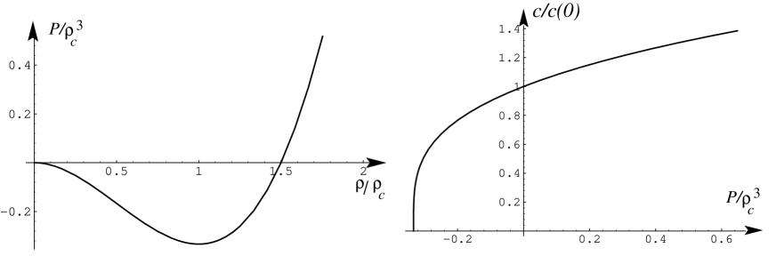
FIG. 1.: Respectively, the pressure as function of the density and the sound velocity as function of the pressure for the model SNLS. These graphs show a consistent liquid-gas transition, where the spinodal decomposition point is located at $\rho=\rho_{c}$.

a) b)

c) d)

FIG. 2.: Density profile for $\delta=3$ and $\sigma=1$ at various time a) for small time, t=0.02, t=0.06 and t=0.12 unit time; the explosion gives rise to a shock wave. b) for t=0.18 and t=0.6; a bubble appears beside the tensile part of the shock wave; oscillating perturbations are emitted by the shock wave. c) for t=2.9, t=7.9 and 13.4; the bubble grows until a maximal radius and begins to retract at t=13.4; the shock wave has changed in a spherical sound wave and is no more moving with the bubble interface. d) t=18.4, t=23.4 and t=24.4 the bubble collapses, giving rise to a secondary explosion. A large part of the energy has been radiated through the spherical waves.

FIG. 3.: Position, as a function of time, of the maximum of the density. It exhibits two typical behavior, one for small time, when the wave is supersonic, the other one later, where the shock wave has transformed in a sound wave (the position evolves then linearly in time). For the small time, the position of the shock wave is consistent with a law $R_{p}\propto t^{1/2}$.

FIG. 4.: The deviation from average density as function of time. After a short transient, this quantity evolves as a power law in time ($\rho_{p}-1\propto t^{-\mu}$). The two lines above the graphs correspond to $\mu=0.5$ for small time and $\mu=1$ later.

FIG. 5.: The over-density as function of time for a huge explosion $\delta=8$ and $\sigma=1$. The line indicates the slope $t^{-1/2}$. The small time behavior coincides with a $\mu=1/2$ regime.

FIG. 6.: Radius of the bubble induced by an explosion as function of time ($\delta=2$ and $\sigma=1$). The growth and the collapse are not symmetric. Both the growth and the collapse obey the Sedov-Taylor law for the radius as function of time.

a) b)

FIG. 7.: a) phase $\phi$ as a function of $\xi$ the self similar variable, for different time (from $t=0.01$ to $t=0.2$; $\delta=8$). Except the two first curves, which correspond to the lowest time, where the dynamics is still in the transient, the different curves almost coincide for $\xi\sim 0$ and have a parabolic shape, as predicted by the simple self similar approach. b) for different $\delta$, $\phi/\delta^{2}$ as function of $\xi/\delta$; according to the self similar analysis, these curves should coincide.

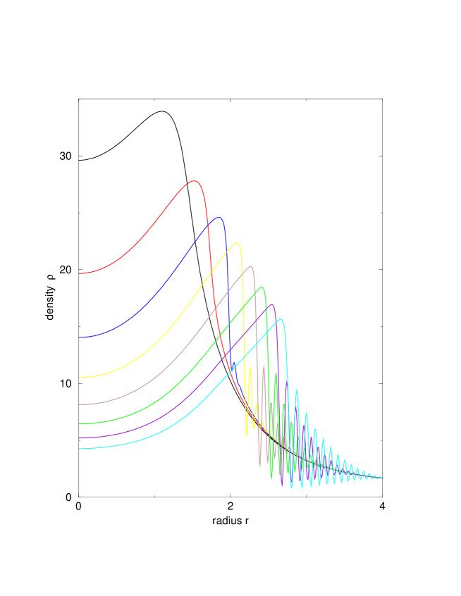
FIG. 8.: density profile of the solution of SNLS for $\delta=8$ and $\sigma=1$ for different time smaller than $0.05$ unit time. One can observe a self similar shape in the shock wave as time goes on. Even if the density obeys a linear profile for intermediate values of $r$, it is not valid anymore for $r\rightarrow 0$.

FIG. 9.: Numerical solution of equation 14 using the shooting method, where $f^{\prime}(0)=0$ and $f(0)=A$. For the lower curve, $A=0.98473178<A_{c}$ and the upper one is for $A=0.98473178435>A_{c}$.

REFERENCES

- [1] S. Hilgenfeldt, D. Lohse and M. P. Brenner, Phys. Fluids 8, 2808 (1996).
- [2] M.S. Pettersen, S. Balibar and H.J. Maris, Phys. Rev. B 49, 12062 (1994).
- [3] S. Balibar, C. Guthmann, H. Lambaré, P. Roche, E. Rolley and H.J. Maris, J. Low Temp. Phys. 101, 271 (1995).
- [4] A.C. Newell and J.V. Moloney, Nonlinear Optics. (Addison-Wesley, Reading, MA, 1992).
- [5] C.E. Brennen, Cavitation and Bubble Dynamics. (Oxford Engineering Science Series 44, Oxford University Press 1995).
- [6] C.D. Ohl, O. Lindau and W. Lauterborn, Phys. Rev. Letters, 80 393 (1998).
- [7] R.A. Wentzell and G.J. Lastman in Cavitation and Inhomogeneities. (Springer Series in Electrophysics 4, Editor W. Lauterborn 1980), p72.
- [8] V.L. Ginzburg and L.P. Pitaevskiǐ, Sov. Phys. JETP 7, 858 (1958); L.P. Pitaevskiǐ, Sov. Phys. JETP 13, 451 (1961); E.P. Gross, J. Math. Phys. 4, 195 (1963).
- [9] C. Josserand, Y. Pomeau and S. Rica, Phys. Rev. Letters, 75, 3150 (1995).
- [10] C. Josserand and S. Rica, Phys. Rev. Letters 78, 1215 (1997).
- [11] L.D. Landau, J. Phys. USSR 5, 71 (1941); ibid. 11, 91 (1947).
- [12] Y. Pomeau and S. Rica, Phys. Rev. Letters 71, 247 (1993).
- [13] L. Onsager, Nuovo Cimento Suppl. 6, 249 (1949).
- [14] L.D. Landau and E.M. Lifshitz, Fluid Mechanics, Chapter 106, Pergamon Press (Oxford) 1987.
- [15] we used a Gauss-Seidel Crank-Nicholson finite difference method to integrate equation 6. We present results obtained for , and for various values of . The number of points of the 1-D mesh did vary from 512 to 2000 and the finite space step varied from to . The number of particles is conserved with a relative accuracy of .
- [16] L.D. Landau and E.M. Lifshitz, Fluid Mechanics, Chapter 70-71, Pergamon Press (Oxford) 1987.
- [17] S. Balibar, H. Lambaré and P. Roche, Private communication.
- [18] Mathematica, S. Wolfram.
- [19] L.-Y. Chen, N. Goldenfeld and Y. Oono, Phys. Rev. E, 54, 376 (1996).
- [20] S. Dyachenko, A.C. Newell, A. Pushkarev and V.E. Zakharov, Physica D 57, 96-160, Part V (1992).
a)  b)
b)
c)  d)
d)
a)  b)
b)