Quantum Hall Effect: Current Distribution and Existence of Extended States

Abstract

We present a consistent description of the current distribution in the quantum Hall effect, based on two main ingredients: the location of the extended states and the distribution of the electric field. We show that the interaction between electrons produces a boundary line below the Fermi energy, which extends from source to drain. The existence of this line and that of a physical boundary are responsible for the formation of a band of extended states that carry the Hall current. The number and density of these extended states are determined by the difference between the energy of this equipotential boundary line and the energy of the single extended state that would exist in an infinite system. This is used to prove that the band of extended states is distributed through the bulk of the sample. We explore the distribution of the Hall currents and electric fields in by presenting a model that captures the main features of the charge relaxation processes. Theoretical predictions based on this model and on the preceding theory are used to unambiguously explain recent experimental findings.

I Introduction

Since the discovery of the quantum Hall effect (QHE) [1] two different approaches have been used to describe it: one focuses on the properties of the edge channels [2, 3], while the other concentrates on the states in the bulk of the system [4, 5, 6, 7, 8, 9]. Both of these approaches associate the quantization of the transverse conductivity $\sigma_{xy}$ in units of $e^{2}/h$, and the absence of dissipation ($\sigma_{xx}=0$) with the formation of an incompressible liquid state in the bulk of the system, and both are based on the existence of delocalized states. However, the nature of the injected Hall current is quite different in these theories. In the first approach [2, 3], which neglects inter-electron interaction, electrons from the current source are injected into delocalized states at the Fermi level which carry the Hall current. Since the only states at the Fermi level are located at the edge of the system (edge channels), the Hall current has to be confined to this narrow region near the sample boundary. The magnitude of this edge current is $ne^{2}/h$ times the difference between the chemical potentials at the two edges of the system. In the latter approach the Hall current density is proportional (with the same constant of proportionality) to the electric field, whose appearance is due to the charging of the system [4, 5, 6, 7, 8, 9]. In this case the Hall current is still the same but it generally flows both along the edge and in the bulk of the system depending on the Hall electric field distribution.

Experimentally, it has proved difficult to determine which of these descriptions is correct, and different probes produce apparent contradictory answers. Measurements of the equilibration rates between the current carrying states [10], as well as experiments on non-local conductivity [11] have natural explanations in terms of edge currents. However, studies of the breakdown of the QHE [12], the direct measurements of the Hall voltage in the sample [13] and recent measurement of electric field distribution [14, 15, 16] favor the picture of bulk currents. It is the objective of this paper to clarify the situation and provide a description of the current distribution in the quantum Hall regime which is consistent with the seemingly opposing experimental results.

It was proved earlier [17] that the Hall current is absent in the regions near the edge where the electron density increases from zero to its bulk value. These are the conventionally defined edge channels. Yet one can imagine the situation when most or all of the current does flow right next to these regions, along their boundaries. Moreover, the existence of the disorder potential modifies the shape and the whole notion of edge channels as they can no longer be thought of as simple homogeneous strips ‘parallel’ to the boundaries.

The complexity of the near-edge as well as of the bulk geometric structure was revealed by recent experiments on imaging the potential distribution in the QH bar at different filling factors [14, 15, 16]. It is worth noting that the relation between the Hall electric field and Hall current in such a complex inhomogeneous system can only be reasonable with some kind of averaging procedure. Local currents are the combination of non-equilibrium Hall current and diamagnetic currents and, in general, it is not possible to differentiate them without averaging over distances of the order of a typical localization length of the closed trajectories. A similar argument holds for the disorder and Hall voltage contributions to the electric potential. Therefore one has to be very careful inferring the Hall current distribution from the measured electrostatic potential distribution. When the Hall voltage is sufficiently large the external electric field smears out some of the disorder potential fluctuations and observation of this electric field distribution on shorter scales becomes possible. However, the state of the QH system in such strong Hall electric field is far from equilibrium, and the information obtained from non-linear regime measurements, although interesting and valuable in itself, does not interpolate into a linear regime (experiments associated with the study of the breakdown of the IQHE produced current-voltage characteristics very distinct from linear at sufficiently high Hall voltages [18, 19]).

The problem of the current distribution in the QH sample is also intrinsically connected with the question of the existence of delocalized states in the presence of disorder. The latter was widely discussed in the literature [20, 21, 22, 23, 24] but was not usually related to the problem of current distribution. Trugman [21] showed the connection between the existence of delocalized states and the classical percolation problem in an infinite system with long-range disorder potential. In his paper [21] and in Ref. [20] the possibility of creation of current carrying extended states by external electric field is discussed. The role of the physical boundaries of the system on the existence of delocalized states was also addressed in Ref. [20]. However, it was still not clear where these delocalized states are located with respect to the physical boundaries of the system, and whether the delocalization due to the applied external electric field is confined to the edges or not.

In this paper we examine the distribution of extended trajectories in equilibrium and use these findings to study the distribution of the Hall current in the bulk. The conditions for the electric field to be concentrated at the boundaries or spread into the sample are found and compared with corresponding experimental values. We find that, in addition to the restrictions put forth in our previous work [17], the Hall current paths are distributed throughout the bulk of the system under the most common experimental conditions. The interplay between the inter-electron interaction and the long-range disorder potential turn out to be crucial in establishing such a current distribution.

The paper is organized as follows. In Sections II and III we discuss the equilibrium state of a Quantum Hall system when no Hall current is present. We prove that there are delocalized states in incompressible regions both near the edges and in the bulk of the sample. Section IV deals with the Hall field and Hall current distributions away from equilibrium. We find that, similarly to the situation in equilibrium, extended states are distributed throughout the sample, their particular spatial density being dependent on disorder configuration and on the rate of relaxation processes. In Section V we discuss the validity of Středa formula [25] in the context of previous arguments. The controversy around the formula is resolved using the arguments of the previous sections. Finally, in Section VI a consistent interpretation of recent experiments is presented. Although the findings of these experiments do not appear to be in complete agreement with the absence of near-edge Hall current, we demonstrate how these results confirm the theory of the distribution of extended states presented in this paper when all the experimental conditions are fully accounted for.

II Compressible and Incompressible Bulk

Consider a typical system where the QHE is observed: a 2DEG formed at the interface of the GaAs/GaAlAs heterostructure, placed in a strong magnetic field $B$, with the length of the system $L_{y}$ being much larger than its width $L_{x}$. In absence of disorder, in the Landau gauge, with vector potential $A_{y}=B\,x$, the electrons are free in the $y$-direction and quantized in the $x$-direction. Wave functions can be written as $e^{iky}f_{n}(x-kl^{2})$, where $l=(\hbar c/eB)^{1/2}$ is the magnetic length and $n$ enumerates the Landau levels (LL’s). In homogeneous systems, wave functions and energies are simply those of the harmonic oscillator: $\epsilon_{n}=\hbar\omega_{c}(n+1/2)$, where $\omega_{c}=eB/mc$ is the cyclotron frequency.

The disorder potential plays a crucial role in establishing the QHE. Two different types of disorder potential, short-range and long-range, require different approaches to elucidate the properties of the 2DEG. The former is realized, e.g. in the MOSFET-devices and InAs heterostructures; it leads to low-mobility samples and is known to produce wide QH plateaus and scaling in the transitional regimes between the QH plateaus even at temperatures above 1 K  [26]. High-mobility samples are formed at the interface of GaAs–Al_xGa_1-xAs heterostructures, characterized by a long-range disorder potential. This potential is created by a Si-ion layer separated from the 2DEG by a undoped spacer with a typical thickness $d\simeq 100-500$Å [27]. In this paper we will be concerned only with this latter type of the systems. In contrast to low-mobility samples, the inter-electron interaction is very important in the case of a long-range disorder potential: electrons tend to screen potential fluctuations whose wave-length $\lambda$ is larger than both the magnetic length (see Refs. [28, 29, 37]). At the same time the finite distance to the donor plane strongly suppresses fluctuations with wavelengths shorter than the spacer thickness [28, 29].

In presence of a strong magnetic field, however, screening is limited by the incompressibility associated with the existence of the gap between the LL’s, and filled LL’s do not contribute to screening. Still, if the filling factor $\nu=\pi l^{2}n_{0}$, $n_{0}$ being the electron density, is not close to an integer, there are plenty of unoccupied states on the top-most occupied Landau level, and the long-range fluctuations of the random potential get screened in a significant part of the sample area [28]. When the filling factor is close to an integer one expects to find regions in which the fluctuations of the random potential are not screened. In these regions some LL’s are completely filled while the rest are completely empty. When a region with $N$ completely filled LL’s percolates throughout the sample the QHE is observed. The number $N$ is usually the integer closest to the average filling factor $\nu$.

Because this percolation picture of the QHE is valid only for filling factors close to an integer, it cannot describe the whole range of magnetic fields where the QHE is observed. Evidently, some other aspects of this problem, not accounted for in this simple picture, lead to the QHE at occupation numbers away from integers. This important issue will be discussed in an upcoming publication [29].

In this work, we restrict ourselves to systems in which the region occupied by the incompressible liquid percolates, and study the current distribution in this percolating region. The potential at every point of the sample is determined by the random distribution of impurities in the dopant layer and by the distribution of the electron charge all over the 2DEG-plane. The potential thus generated has only relatively long-wavelength variations, and this, combined with the strong magnetic field, allows for the following simplification: electrons can be considered drifting along the lines of the constant classical energy [30]. The Hall current injected into the sample is therefore carried by the electrons moving along the trajectories stretching from source to drain. Thus, there are two factors that eventually determine the spatial distribution of current in the sample: the steady state charge and Hall electric field distributions, and the location of the extended (i.e. percolating from source to drain, the definition which we will be using throughout the paper) classical trajectories. To study these properties in the steady state, we first address the same questions for the equilibrium state of this 2DEG system.

III Extended trajectories and diamagnetic current distribution in equilibrium

In this section we develop a consistent description of the current carrying states in equilibrium. It is proven that extended states are present both deep in the bulk of the sample and close to its edges.

A Edge channels in presence of disorder: definition and absence of Hall current

Let us consider an infinite two-dimensional random potential. It is clear from percolation theory that all equipotential lines but one are closed [20]. As a corollary we find that in an infinite 2DEG in a strong magnetic field for each LL there is a single energy $E_{i}$ such that the state with this energy is extended in both directions. The only percolating equipotential line corresponds to this extended state (one per each LL). If a finite-size system were equivalent to a piece of the same size in the infinite system (with no inhomogeneities introduced by the boundaries), a band of states around $E_{i}$ whose localization length is larger than the sample size, would appear as delocalized. However, in the finite size sample these states can percolate only in one direction, namely, the shorter one [20]. The simple assumption above produces a drastic consequence: there are no extended states in the longer $y$-direction, and we should expect no Hall current in this direction (Fig. 1a). It is clear that the boundaries produce a non-trivial effect.

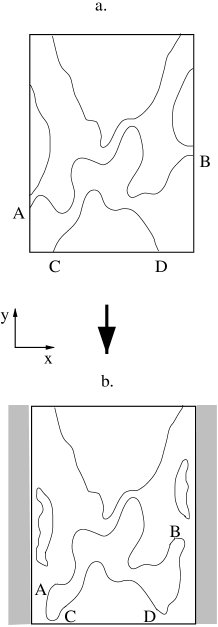
FIG. 1.: Finite size effects on the extended states. a. Elimination of percolation in the longer $y$-direction. Trajectory $AB$ is one from the band of the states percolating in x-direction; line $CD$ is part of a closed trajectory in the corresponding infinite system. b. Effects of a confining potential: lines $AB$ and $CD$ link to each other to become a single closed equipotential line. Other trajectories are also deformed by the confining potential.

In reality, the 2DEG is confined in the shorter $x$-direction by a self-consistent potential created by the positive background, electron charge distribution, and gate voltages. Such a potential leads to an increase of the density of electrons from zero at the physical edge of the 2DEG to the bulk value. Depending on the sharpness of the confining potential such growth can be either gradual or step-like [31, 32]. For illustrative purposes, let us assume that the charge density grows gradually (but the arguments that follow are valid in either situation). In this case, a narrow compressible region with a partially filled LL percolating in $y$-direction is formed near the edge [31]. In this region the variations of the potential due to confinement and disorder are largely screened by electrons. As long as there are enough unfilled states on the same LL, electrons can screen variations of the potential. The density profile $n(x)$ in the 2DEG at the edge is approximately given by the electrostatic solution [31]

$$n(x)=\left[\frac{x-l}{x+l}\right]^{1/2}n_{0}\,,\,\,\,x>l.$$ (1)

Here $x$ is the distance from the physical boundary of the 2DEG and $l$ is the width of the depletion layer. However, as the occupation number of the first filled LL grows as required by the electrostatic solution (1), less and less ‘space’ is available for variations of the local electron density, and consequently, more and more variations of the potential are left unscreened. Finally, as we move towards the bulk of the system, the electrons completely loose the ability to screen the potential fluctuations, and these unscreened regions link to form a continuous strip of incompressible liquid along the $y$-direction. The outermost incompressible strip corresponds to a single filled LL. Moving further away from the edge, the potential starts falling. If more than one LL are filled in the bulk, the potential drops by $\hbar\omega_{c}$ in each incompressible strip, and then another compressible river (with partial occupation in the next LL), is formed roughly parallel to the $y$-direction [31]. When the last ($N$-th) LL becomes completely filled, the fall of potential is entirely due to the unscreened fluctuations of the disorder potential (Fig. 2b). Note that while a purely electrostatic solution in the absence of disorder predicts a complete screening in the bulk for any filling factor, the situation is, in fact, considerably different due to the interplay of disorder and LL quantization.

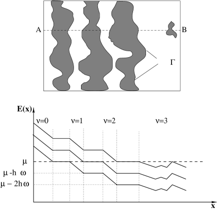
FIG. 2.: Charge distribution and energies of Landau levels near the physical boundary a. Compressible and incompressible ‘strips’ near the edge. b. Energies of the first three occupied Landau levels close to the sample boundary.

We conclude that at the left edge of the sample there is a geometric boundary line $\Gamma$ which ought to be infinite in the $y$-direction, and which marks the transition from the last compressible strip to the incompressible bulk (Fig. 2a). To the left of this line the density of the electron charge falls off, and there are $N$ percolating compressible strips. We will refer to this region from the physical edge of the system to the boundary line $\Gamma$ as to the ‘edge channel region’ (there are two such regions – one at each edge as the argument above clearly holds for the right edge, as well). On the other side of this boundary, an incompressible region with $N$ completely filled LL’s percolates. In this region the potential falls due to the unscreened fluctuations of the disorder potential (Fig. 2b). To this whole region we will refer to as the bulk.

Let us first show that in the regime of the QHE no part of the non-equilibrium Hall current flows in the edge channel region as defined above (for a more detailed discussion see Ref. [17]).

In equilibrium, although the net current is zero, orbital current flows along the trajectories extended from source to drain at one edge and in the opposite direction at the other edge. There are two contributions to this equilibrium current which are spatially separated [33]. First, the diamagnetic current, is roughly proportional to the gradient of the self-consistent confining potential, and it is non-zero only in the incompressible regions. The other one is associated with the concentration gradient, which is different from zero only in the compressible strips close to the device boundary. However, the total current carried by the partially occupied near-edge region of the $n$-th LL is always $(n+1/2)e\omega_{c}/2\pi$, independent of the external conditions [33]. Corresponding compressible strips at opposite edges of the sample carry the same current but in opposite directions, therefore only incompressible regions can support non-equilibrium current. This can also be seen from classical considerations: non-equilibrium Hall current is carried by electrons drifting in crossed electric and magnetic fields in the direction perpendicular to both of them. This drift velocity is proportional to the local electric field, which is identically zero in the compressible regions. We will, therefore, ignore the current in the compressible regions (even if extended trajectories are present there) since it is not changed by the injected non-equilibrium current.

Consider now the case when current is injected into the sample. Under conditions of the QHE, the longitudinal conductivity is negligible, and there is no dissipative current between the two edges. Therefore, for every value of the injected current smaller than the critical current corresponding to the QHE breakdown, there exists a many-particle steady state that carries the current. This non-equilibrium steady state can be described by certain charge and current distributions in ways similar to an equilibrium state. The only difference is that in the steady state the net current in the transverse direction is different from zero. As a consequence of this, LL’s are filled up to different energies at the left and the right edges, and a Hall voltage can be measured. As the non-equilibrium current is carried by the states in the incompressible regions, the total current flowing in the sample can be obtained by summing over the contributions due to the electrons in the fully occupied extended states.

Let us first compute the total amount of current carried in the edge channel region. Following Trugman [21] we calculate the Hall current carried by one LL through some horizontal cross section $y=y_{0}$ of length $\triangle L=x_{2}-x_{1}$ along which the potential falls by $\triangle V=V_{2}-V_{1}$. The number of electrons per unit area $n$ is equal to $1/2\pi\hbar l_{b}^{2}=eB/hc$. Define the expectation value of the local electron velocity operator at each point along the line $x_{1}x_{2}$ [21]:

$$<\vec{v}(\vec{r})>=c\,\frac{\vec{\cal E}(\vec{r})\times\vec{B}}{B^{2}},$$ (2)

where $\vec{\cal E}(\vec{r})$ is the electric field. The current $I_{x_{1}x_{2}}$ that passes through the line $x_{1}x_{2}$ is:

$$I_{x_{1}x_{2}}=\int_{x_{1}}^{x_{2}}\!dx\,ne\,(\vec{v}\cdot\hat{y})=-\frac{e^{2}}{h}\,\frac{V(x_{2},y_{0})-V(x_{1},y_{0})}{e}.$$ (3)

Since local currents, circulating in the closed trajectories, contribute neither to total diamagnetic current nor to non-equilibrium Hall current (we will study their importance in Section V), let us choose the points $(x_{1},y_{0})$ and $(x_{2},y_{0})$ on the extended trajectories at potentials $V_{1}$ and $V_{2}$ respectively. Then the strip between these two trajectories contributes the amount proportional to $\triangle V=V_{2}-V_{1}$ to the total current as given by Eq. (3).

The Hall conductivity is $\sigma_{xy}=I/V_{H}$, where $V_{H}$ is the Hall voltage measured in the four-terminal resistance experiments. This voltage is determined by the amount of current carried by each LL just before the voltage contacts, as well as by the transmission and reflection coefficients of these contacts. It is possible to show [3] that the Hall conductivity will be quantized only if, upon leaving the voltage contacts, all LL’s are filled up to the same energy: $\epsilon_{n,l}=\mu_{1}$, $\epsilon_{n,r}=\mu_{2}$ for all $n$. In this case, the voltmeter measures the difference between the chemical potentials at the two edges: $V_{H}=(\mu_{2}-\mu_{1})/e$. Then from Eq. (3) follows that $\sigma_{xy}=Ne^{2}/h$. We must note at this point that filling of each LL starts when the energy of this LL drops to $\mu_{1}$ ($\mu_{2}$) at the left (right) edge. This means that all partially occupied states at one edge have the same energy ($\mu_{1}$ or $\mu_{2}$). Then, both in equilibrium and in the non-equilibrium steady state described above, the total drop of the potential $\triangle V_{n}$ in the part of the edge channel region where the $n$-th LL is filled, equals to $(N-n)\hbar\omega_{c}$. Therefore, the potential falls by $(n-1)\hbar\omega_{c}$ before the $n$-th LL starts to fill, and by $(N-1)\hbar\omega_{c}$ through the whole edge channel region. As the energy difference between the LL’s in the compressible strips does not change when the current is injected, the total potential drop $\triangle V_{n}$ is also not changed by the injection of the Hall current. It follows then from Eq. (3) that the current flowing in the edge channel region is always equal to the equilibrium diamagnetic current, even when the non-equilibrium current is injected into the sample. In other words, no non-equilibrium current flows in the edge channel region, and the entire injected current is carried by the states in the bulk of the system, to the right from the line $\Gamma$ on Fig. 2a (see also Ref. [17]). The rest of the paper discusses the distribution of the extended trajectories in the bulk of the sample.

It is important to realize that the complete equilibration at the edge leads, therefore, to complete absence of non-equilibrium current in traditionally defined edge channels. On the other hand, if this equilibration is not perfect, some portion of the non-equilibrium current is pushed into the edge channels. However, in this case, the measured Hall conductance is not quantized in units of $e^{2}/h$. Experiments, involving non-ideal contacts [10] (contacts designed to avoid complete equilibration) clearly demonstrated this absence of quantization and implied presence of currents in the edge channels. In fact, partial equilibration was still achieved in such experiments due to inter-channel scattering. It was argued, however, that the only source of perfect equilibration are the ideal voltage contacts [17]. We argue, additionally, that employing the ideal contacts leads necessarily to the absence of non-equilibrium current in the edge channels. Therefore, the experimental conditions are crucial in determining the Hall current distribution.

B The extended states, a continuity theorem

Here we determine the spatial location of the extended states under QHE conditions. Let us consider the behavior of the potential immediately to the right of the line $\Gamma$. As mentioned above, this potential initially falls due to the incompressibility in this region (see Fig. 2b). Exactly how far the potential falls depends on the local configuration of the random potential, and at some point the potential will necessarily start raising again. Therefore, there is a spatially extended region to the right of $\Gamma$ where the potential falls. Since $\Gamma$ itself is an equipotential line at energy $\epsilon_{\Gamma}=\mu-N\hbar\omega_{c}$, by continuity there is a finite range of energies $\epsilon_{\rm last}<\epsilon<\epsilon_{\Gamma}$ in which equipotentials percolate in the $y$-direction. Here we denoted the lowest energy of these equipotentials by $\epsilon_{\rm last}$ and the chemical potential by $\mu$. We now ask what determines this minimum energy $\epsilon_{\rm last}$ and the shape of the corresponding equipotential. The results are far from obvious.

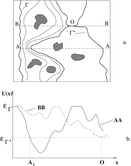
FIG. 3.: Extended trajectories from the edge towards the bulk of the sample a. Open trajectories: $\Gamma$ is the inner boundary of the edge region, $\Gamma^{\prime}$ is the last open trajectory in the bulk. b. Corresponding energy profiles along the marked cross section lines AA and BB.

It was argued before that in the absence of the confining effects of the physical boundary (we will call such an artificial construction a ‘quasi-infinite system’), the only effect of the finite size in $x$-direction would be the existence of a narrow band of equipotentials connecting left and right edges. Let us assume that an equipotential $\Gamma^{\prime}$ with energy $\epsilon_{0}$ belongs to this band. It is useful to note that at this energy there may also be other trajectories that do not percolate. Going back to a more realistic system, with confining potential at the edges, one can see that this percolating trajectory $\Gamma^{\prime}$ is necessarily cut off by a rise of the potential towards the physical edge (Fig. 3). It is then easily seen that at each energy between $\epsilon_{0}$ and $\epsilon_{\Gamma}$ there exists one and only one equipotential line open in $y$-direction, and that no trajectory at energies lower than $\epsilon_{0}$ can percolate vertically.

Proof: Let us connect lines $\Gamma$ and $\Gamma^{\prime}$ by means of an arbitrary line $\gamma$. Along this line the potential has to fall from $\epsilon_{\Gamma}$ at $\Gamma$ to $\epsilon_{0}$ at $\Gamma^{\prime}$. The potential along the $\gamma$ line does not have to be monotonous.

a. Let us initially assume that the potential is monotonous along $\gamma$. Now connect $\gamma$ with the left and right edges by, say, horizontal straight lines $AA_{1}$ and $BB_{1}$ (Fig. 4). Choose any point $P$ on $\gamma$ between $A$ and $B$. We now ask whether an equipotential line threading through $P$ percolates in the $y$-direction. In order for the trajectory passing through $P$ to be a closed one, one has to find another point on the line $A_{1}B_{1}$ with the same potential as in point $P$. Such point cannot be found on $\gamma$ because of the monotonous behavior of the potential along it. There could be such points on the piece $BB_{1}$ but in order to reach them one has to cross line $\Gamma^{\prime}$ which is at different potential. Hence, there is no way to close equipotential trajectory by going to the right of $P$. A similar argument shows that one cannot close trajectory to the left from $P$ either. Therefore, the equipotential passing through any point on $\gamma$ is necessarily delocalized in the $y$-direction.

b. Going back to the general case of a non-monotonous potential on $\gamma$, we argue that for any energy $\epsilon$ such that $\epsilon_{0}<\epsilon<\epsilon_{\Gamma}$ there will be an odd number of points on $\gamma$: namely, there will be one more point on the fall of potential than on the rise. Some of these points combine pairwise into closed orbits. However, the additional single point satisfies conditions similar to those stated in part a: the equipotential passing through it must be extended in the $y$-direction.

From this discussion it is also clear that no trajectories with energies beyond the interval $[\epsilon_{0},\epsilon_{\Gamma}]$ can percolate in $y$-direction.

FIG. 4.: Illustration of the proof of continuity theorem.

We immediately recognize that $\epsilon_{0}=\epsilon_{\rm last}$ and that the corresponding right-most vertically percolating equipotential is the line we denoted $\Gamma^{\prime}$ on Fig. 3. Therefore, as a first approximation, the trajectory $\Gamma^{\prime}$ has to percolate in both vertical and horizontal directions. This is a critical trajectory with at least one saddle point $O$ on it. An equilibrium picture of extended trajectories emerges according to this discussion as shown in Fig. 3.

Qualitatively, we conclude that at least the trajectories with energies greater than, but sufficiently close to $\epsilon_{0}$, travel throughout the system towards the ‘saddle point’, as does the critical trajectory itself. The latter comes near the boundaries only to get around closed trajectories with similar energies and with large sizes in the $x$-direction. Since such trajectories are very sparse, the critical trajectory spends most its path inside the system rather than near the boundary. In addition, there can also exist vertically percolating trajectories in the edge compressible regions to the left of line $\Gamma$ (see Fig. 2).

C General remarks

Insofar, by means of purely geometrical arguments, we have proved that:

i. Contrary to a widespread belief, it is not just the existence of the physical boundaries which is responsible for the formation of a band of extended states (instead of a single extended state in the infinite random two-dimensional system). It is clear from the preceding discussion that the number, density and location of the trajectories extended in $y$-direction have little to do with the sample size in $x$-direction. This is in complete contrast with the common statement that the bandwidth of the extended states is inversely proportional to the sample size. The most important factor is the interaction between electrons which leads to the screening of the confining and disorder potential at the physical boundary and, consequently, to the formation of an extended boundary line $\Gamma$. It is the difference between the energy of this equipotential line $\Gamma$ (which is equal to the chemical potential $\mu$) and the energy of the state extended in a corresponding infinite system, that determines the total number and density of extended states in equilibrium.

ii. In addition, we must conclude that even in equilibrium, extended states are present not only near the physical boundary but also deep in parts of the bulk, their particular, sample-dependent distribution being determined by a specific configuration of the disorder.

In the next section we give a detailed description of how, under the conditions of complete equilibration at each edge, the Hall current is distributed in the sample.

IV Delocalized trajectories and current distribution in the steady state

Imagine going from the line $\Gamma$ towards the inside of the system in the current carrying steady state. The difference from the equilibrium state then is that the counterpart of $\Gamma$ at the right edge is an equipotential at an energy lower than $\epsilon_{\Gamma}$ by the Hall voltage $V_{H}$. Using arguments similar to the ones applied in equilibrium, it is easy to demonstrate that there is a critical trajectory $\Gamma^{\prime}$ with at least one saddle point in the steady state. The energy of this critical trajectory will not be the same as in equilibrium: in our setting of Hall field directed from right to left, the following inequality should hold: $(\epsilon_{\Gamma}-\epsilon_{\Gamma^{\prime}})_{\rm non-equil}>(\epsilon_{\Gamma}-\epsilon_{\Gamma^{\prime}})_{\rm equil}$. Therefore, the number of extended trajectories differs from the one in equilibrium. This should be true independently of whether the charge distribution is changed due to the presence of Hall electric field or not.

As the Hall current is injected into the sample, it charges the edge metallic regions establishing the chemical potential difference between the two opposite edges. These charges produce the long-range electric field decaying as the inverse distance from each edge sufficiently far from this edge [6, 7, 34, 35]. In the context of the problem of Hall current distribution the effect of charged edges was thoroughly studied in the past [6, 7, 34]. If these charges cannot move into the bulk they create a logarithmic potential sufficiently far from the edges. This solution assumes zero longitudinal conductivity. More realistically, however, one has to estimate the charge relaxation times associated with the finite longitudinal conductivity $\sigma_{xx}$ or with some other charge relaxation mechanisms (not related to the transport by the extended states) . Thouless [34] considered a finite $\sigma_{xx}$, and assumed as the condition for a steady state a constant value of dissipative current $j_{x}(x)={\rm const}$. The problem reduces to the two-dimensional Poisson equation and is solved for the charge distribution inside the Hall bar. This new charge distribution produces a homogeneous electric field across the sample and can be established only if there are regions in the bulk which can absorb additional charges. The origin of such regions, their sizes and spatial distribution will be discussed at the end of the paper in the context of recent measurements, and for the estimates of typical charge relaxation times. A more thorough treatment can be found in other publications [29, 37, 36].

Consider first the situation when the relaxation time is very long compared with the time of measurement. In this case the Hall electric field is negligible at the saddle point on the critical trajectory, falling off inversely with the distance from the edge. One can argue that this critical trajectory changes its energy but the saddle point on it does not move. Consequently, all the newly formed percolating trajectories have to be located between the critical trajectory and the adjoining edge region, that is, in the region where delocalized states were present in equilibrium. Similarly to equilibrium delocalized trajectories, the newly formed ones are not distributed homogeneously. While in most of the area of the sample their average concentration follows the Hall electric field (by the arguments used to prove the equilibrium distribution), in the regions where the critical trajectory approaches the edge, the density of newly formed delocalized states has to be much higher.

Consider a horizontal cross section $AA_{1}$ where the critical line $\Gamma^{\prime}$ approaches the line $\Gamma$ at a distance $\Delta\ll W$ (Fig. 5). The fall of the potential $\triangle V$ on the distance $\Delta$ due to the external field is negligible compared to the Hall voltage. Yet, the application of a small Hall field cannot destroy many localized states inside the critical trajectory as in most parts of the system the localizing disorder field is much greater than the external one. These two facts can be reconciled if most of the newly formed delocalized trajectories with energies in the interval of the order of $V_{H}$ appear in the narrow neighborhood of the original position of $\Gamma^{\prime}$, to the right of it. The trajectory $\Gamma^{\prime}$ itself shifts to the right by a distance $\delta$ to let the vertically percolating trajectories penetrate into the interval $AA_{1}$ with length $\delta$ (Fig. 5). Such a solution is possible due to the fact that the slope of the potential in the interval $AA_{1}$ is determined by the field of disorder potential rather than by the much weaker external field. In the areas of the sample where the critical trajectory is sufficiently far from the edges so that the Hall field near this critical trajectory is negligible, the geometry of the critical line does not affect the position of the field-induced delocalized states. The concentration of latter ones follows the intensity of the Hall field and the concentration of equilibrium extended trajectories: new trajectories are formed as a response to the Hall electric field on those slopes of disorder potential which contained delocalized states in equilibrium. One concludes, therefore, that, except for the electrostatic Hall electric field, there are no specific features brought into the Hall current spatial distribution by the edges. Since equilibrium delocalized trajectories are generally not concentrated near the edge (previous Section), neither are the newly formed ones. The density of non-equilibrium extended trajectories is weighted towards the edges only to the extent the Hall electric field is.

FIG. 5.: Critical trajectory $\Gamma^{\prime}$ approaching the boundary line $\Gamma$ and the form of electrostatic potential in this region (see the text).

The other limiting case is the condition of complete (fast) relaxation. It is realized if the charges, including those on localized states, respond to the external electric field created by the charged edges and redistribute themselves according to the steady state solution. The typical rate of this response must be greater than the rate at which the parameters are changed in the experiment. The only possible source of charge redistribution are the metallic regions of partially filled Landau levels. Therefore, one has to estimate the time it takes for a finite charge to be transfered from any such metallic region to the neighboring one.

There is experimental evidence that, in many circumstances, equilibration does occur. Direct study of relaxation processes [38] shows that the state of an incompressible system achieved by raising the magnetic field from zero to several Tesla at high temperature (of the order of 1K) differs significantly from the one reached by increasing the magnetic field in a pre-cooled (100mK) sample and then heating it up back to 1K. Although the relaxation considered in [38] requires spin-flip processes and is, therefore, significantly slower, one can think of the relaxation as being facilitated by higher temperatures allowing for greater hopping or activated current.

Other group of experiments produce some indirect evidence of relaxation: the dependence of QH breakdown current on the sample width. Most of these measurements show a linear dependence which contradicts the assumption that the current flows primarily through the edges. This implies that that the electric field is close to a constant across the sample. This can be achieved only by delivering electrons to localized states in the compressible islands. At currents close to the critical current for breakdown of the QHE the Hall electric field is comparable with the field of disorder [39] and this factor itself can initiate effective relaxation processes via possible tunneling into unoccupied states on the higher Landau level [40]. However, right before the breakdown, the bulk of the system is a well-defined incompressible system, in which relaxation processes are fast. We will present a consistent theoretical description and quantitative conclusions in the next Section.

Consider now where the delocalized trajectories are located in such an equilibrated system in a weak Hall electric field. The picture of extended trajectories is changed relative to the situation of an insulating (rigid) bulk only by the fact that the electric field is homogeneous on average rather than weighted towards the edges. This difference, however, leads to the distribution of extended states being on average a copy of such a distribution in equilibrium. Therefore, the current injected into the system in such case flows in the region between the lines $\Gamma$ and $\Gamma^{\prime}$ as they were defined in equilibrium and has no preference of the edge regions. In the other words, the current is distributed throughout the system.

V Implications of current distribution

In either of the two limits of short or long relaxation times, for sufficiently small Hall currents, one can label the corresponding regime as ‘linear response’. In such a ‘linear response’ regime the critical trajectory $\Gamma^{\prime}$ plays the role attributed in the edge-channels formalism to the innermost boundary of the edge channels. However, unlike the edge channels, $\Gamma^{\prime}$ itself is not confined to be near the physical boundaries. In this sense the description proposed here is complementary to the edge state formalism. It also resolves some controversy around the validity of Středa formula [25].

In the derivation of the Středa formula it is assumed that the derivative $(\partial n/\partial B)_{\mu}$ is quantized due to the existence of the gap in the density of states between Landau levels. In this formula $n$ stands for the density of states, $B$ for magnetic field, and $\mu$ for the fixed chemical potential. This assumption is crucial for the use of the Maxwell relation $(\partial n/\partial B)_{\mu}=(1/A)(\partial M/\partial\mu)_{B}$, where $M$ is the magnetization and $A$ is the total area of the system. Under certain assumptions (which we mention below) the derivative in the right-hand side is equal to conductivity thus providing the proof for the conductivity quantization. It is clear, however, that there is just a mobility gap between LL’s but there is a finite density of localized states in this mobility gap. These localized states have to contribute to the derivative $(\partial n/\partial B)_{\mu}$ in one way or another. This immediately questions the validity of the assumptions used to prove the equality $\sigma_{xy}=(1/A)(\partial M/\partial\mu)_{B}$ , namely that the change in magnetization $\delta M$ is entirely due to additional edge current associated with the change in chemical potential $\delta\mu$.

For interacting electrons, however, $\delta M$ is constructed from both drift along extended equipotentials and circulating currents on closed loops. The latter ones do not contribute to the Hall conductivity but turn out to be essential in evaluating both right– and left-hand sides of the Maxwell relation [41]. Our argument makes use of the existence of states in the mobility gap, on the one hand by implying the formation of ‘new’ extended trajectories within this gap and on the other, by explaining how these new extended trajectories become responsible for the total change in magnetization.

At higher Hall voltages one expects the original topology of states to be gradually destroyed by the external field. The profile of the random potential has to change to absorb more delocalized trajectories than it would be able to absorb in any of the two scenarios described above. In fact, only at rather strong Hall currents does the treatment presented in this Section need to be reconsidered. It happens only when the relaxation processes and the dissipative transport change significantly compared to the linear response regime. This, in turn, occurs when the local Hall electric field, at least in some areas of the sample, becomes comparable with the electric field of the disorder potential. This field turns out to be of the order of $0.1\hbar\omega_{c}/l_{B}$. The corresponding to Hall current densities are $10$A/m which exceeds experimental values in most cases. At such strong external fields the system becomes more homogeneous as the potential fluctuations get wiped out. The newly formed percolating trajectories spread away from the critical line $\Gamma^{\prime}$ and distribute throughout the sample.

VI Interpretation of Recent Experiments

A theoretical model which captures most of the qualitative and quantitative features of charge relaxation processes in the QH regime has been constructed in Refs. [36, 37]. Here we will sketch the main blocks of the model and present the results leading to a consistent explanation of the two recent experiments [14, 15]. Here we concentrate on the experiments of Ref. [15].

The random resistor-capacitor network model (RRCNM) is based on the theory of charge transfer between isolated metallic islands in the bulk via hopping. Due to the small size of these islands one has to take into account the Coulomb blockade effects: adding or removing a single electron from the island costs a non-negligible charging energy. Therefore, each island serves as a capacitor in the model. Typically the charging energies are of the order of $1$ meV. Moving electron from a charged island to an adjacent neutral one leads to either emission or absorption of a phonon with the energy equal to the difference of the charging energies of the two islands. This difference is typically $0.3-0.5$ meV, or $3-5$ K. Such phonon-assisted hopping is somewhat suppressed, in a case of phonon absorption. However, in the range of temperatures between $300$ mK and $3$ K in which most of the experiments on current distribution and charge relaxation are performed, this suppression is not dramatic.

The other factor limiting the rate of charge transfer through the bulk is the distance between the communicating islands. The extent of the wave function of an electron at the boundary of a compressible island is of the order of a few magnetic lengths. If the distance between the islands significantly exceeds this width, the overlap between the states participating in an individual act of hopping is exponentially small leading to a vanishing hopping probability. This limitation defines a few (if any) paths which are available for a charge transfer. Note that this process not only leads to a finite longitudinal current but also to the formation of a new steady state with a charge distribution different from the one in equilibrium. The links between the islands enter into the model as resistive elements.

The average distance between adjacent islands varies substantially with the filling factor. In the range of temperatures mentioned above, the QH plateau is quite narrow: it spans just $5\%$ to $20\%$ of the entire distance between the Landau levels on the scale of filling factors. The greater the number of filled LL’s, the narrower the plateau and the smaller the typical distance between the compressible islands. It turns out that relaxation can be very slow for the filling factor $\nu=2$ (spin-unresolved LL’s) at $T\simeq 300$ mK. However, for $\nu=4$, even at these low temperatures the RRCNM predicts relaxation times of the order of $1$ ms which is shorter than the typical experimental time scales.

The basic block of the simplest RRCN is shown on Fig. 6. Each node corresponds to a compressible island which is connected resistively to a neighboring one. The capacitance of each island to the ground is accounted for by the capacitors $C_{i}$ while mutual capacitances between the islands $i$ and $j$ are denoted as $C_{ij}$.

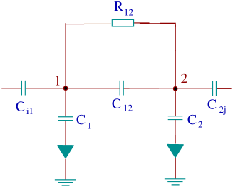
FIG. 6.: The basic block of the random resistor-capacitor network.

The RRCNM is solved numerically for each particular configuration of disorder and at different filling factors. The solution provides the geometric paths of electron transfer, the charges on compressible islands, AC and DC responses of the system, and charge relaxation time $\tau$. Given the conditions of an experiment, one can obtain these characteristics to predict or explain the observed results.

In recent measurements [15], the atomic force microscope technique has been used to study the distribution of the Hall current in the QH sample. Their results which we interpret below, are shown on Fig. 7.

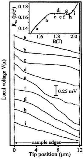
FIG. 7.: Voltage profiles across a 12 $\mu$m-wide Hall bar on a low-mobility sample near the $\nu=6$ QH plateau (traces offset for clarity). The B-fields at which the profiles were measured, and the $\nu=6$ plateau measured by transport are shown in the inset. (a) Well below the plateau, the Hall voltage profile is linear. (b,c) As the plateau is approached, the bulk retains a linear profile but decouples from the edges. (d-g) Well inside the plateau, the profile in the bulk becomes complicated and changes rapidly with field. (h,i) A linear profile returns upon leaving the plateau. [after Ref. [15]]

The scheme of this experiment is different from the one discussed in section III A. This is not a transport-type measurement which means that there are no voltage contacts attached to the sample. The voltage profile is measured capacitively, without a direct contact with the 2DEG. Therefore, the arguments of the section III A proving the absence of non-equilibrium Hall current in the edge channels, will not apply to this experiment in general. More specifically, there is no ideal equilibration between the edge channels provided by the voltage contacts in transport measurements. The only source of inter-edge-channel equilibration is the mutual scattering of electrons [31]. It is less effective than the equilibration in the voltage contacts but for sufficiently narrow edge channels it still leads to the establishment of equal chemical potentials in the compressible edge regions of different LL’s.

On Fig. 7 the results of Hall resistance $R_{xy}$ measurements are plotted. The curve 7(a) corresponds to a filling factor $\nu\simeq 6.8$. The bulk is clearly a metallic system. There are three (spin-degenerate) compressible edge channels ($0\!<\nu<\!2$, $2\!<\nu<4$, and $4\!<\nu\!<6$) and three incompressible edge channels ($\nu\!=2,4,6$). As shown in Ref. [31], only the inner-most edge regions can be wide – up to $10l_{B}$. Since the resolution of the experiment is about $20l_{B}$, the edge regions, whether they are equilibrated or not, cannot be resolved. This leads to a linear profile of the Hall voltage.

As the QH plateau $\nu=6$ is approached with the increasing magnetic field, the bulk filling factor decreases. On the curve 7(b) the bulk filling factor is $\nu_{0}\simeq 6.2$. The filling profile is sketched on Fig. 8. One can use the electrostatic solution for the 2DEG density at the edge, Eq. (1), to estimate how fast the top-most 7-th LL gets filled to its bulk value. Assuming for the depletion width $l$ the typical value $l\approx 10l_{B}$, we find that, for $\nu_{0}=6.2$ the distance between the line with $\nu=6.0$ (point 2 on Fig. 8) and $\nu=6.1$ (point 3 on the same picture) is approximately $300l_{B}$ compared to just $10l_{B}$ for $\nu_{0}=6.8$. Both experimental evidence of the final widths of QH plateaus and our numerical simulations [29] clearly demonstrate that the system remains incompressible in a certain range of filling factors $\triangle\nu$ around the integer. Given the parameters used in these experiments (mobility $80000$ cm²/Vs, density $2.8$ x$10^{11}$ cm^-2 and temperatures between 0.7-1.0 K), according to our numerical simulations (details of which can be found in Ref. [29]), $\triangle\nu\geq 0.1$. Therefore, on a length of the order of $300l_{B}$ to the right from point 2 on Fig. 8 the system is still incompressible. Such a wide incompressible strip makes mutual equilibration between the inner-most compressible edge channel ($4<\nu<6$) and the outer-most states of the compressible bulk practically impossible. To find out where the Hall voltage accumulates one has to study local longitudinal conductivity $\sigma_{xx}$. Since the bulk is metallic, its $\sigma_{xx}$ is quite large (typical metallic conductivity is of the order of $0.1e^{2}/h$). On the other hand, the longitudinal conductance of a wide incompressible strip is exponentially small. The Hall current flows in the region with smaller dissipative conductivity. This explains the observation on Fig. 7(b),(c) of large potential drops near the edges.

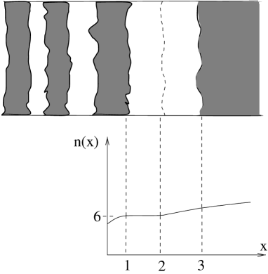
FIG. 8.: Interpretation of the experiment in Fig. 7 (Ref. [15]). The structure of the 2DEG near the edge. Top: alternating compressible (shaded) and incompressible (blank) regions. Bottom: filling factor profile. The dashed line on the top picture and point 2 on the bottom correspond to the distance where the top-most 8-th LL starts filling according to the electrostatic solution [31]. In reality, the preceding incompressible edge channel with $\nu=6$ extends deeper into the bulk (point 3) due to the presence of disorder (see the text).

As the bulk filling factor approaches $\nu_{0}=6$ even closer, the bulk becomes less and less conductive and the incompressible edge region gets wider (eventually connecting the two edges and transforming the bulk into the incompressible state at $\nu_{0}\approx 6.1$). This leads to a smooth transition from an almost linear potential profile across the entire sample Fig. 7(d),(e) to a regime where the potential is flat at the edges and falls only in the bulk (Fig. 7(f),(g)). The profile of the potential in the last regime confirms two conclusions we have made earlier in this paper. The linear fall of the potential in the bulk means there is a complete charge relaxation. In fact, the numerical calculations based on the RRCNM predict relaxation times of the order of $10^{-5}$s for the experimental conditions. This is by far the shortest time present in the problem. Second, oscillations of the curves around the linear profile are caused by the inhomogeneities in the bulk: a linear average electrostatic potential is produced by the charged metallic islands which vary in size and in separation from each other.

VII Conclusions

We have proved, by means of purely geometrical arguments, that a band of extended states, extended from source to drain, results from the interplay between electron interactions and random and confining potentials. These delocalized states extend through the bulk of the system (see Sec. III C).

Based on these conclusions we built a consistent description of the delocalized states in the regime when classical percolation theory is applicable. We were able to demonstrate that, under the most general conditions, the Hall current-carrying states are distributed in the bulk of the Hall sample rather than confined to the edge region. We showed how particular experimental conditions influence the results of the measurements, and yet confirm the general picture of distributed Hall currents. We believe that the controversy regarding the Hall current distribution, as well as the nature and location of extended states in the quantum Hall system is now resolved.

The low temperature regime, however, still needs to be addressed since the equivalence between equipotentials and electron trajectories is lost when quantum effects become essential (for an extended discussion on the transition between the two regimes see Refs. [29, 42]). The authors do not know of any experiment on the distribution of the Hall current and electric fields which explores this low temperature regime. Theoretically a more complete understanding of the microscopic structure of disordered quantum Hall liquid is necessary to solve this problem.

- [1] K. von Klitzing, G. Dorda, and M. Pepper, Phys. Rev. Lett. 45 449 (1980).
- [2] B. I. Halperin, Phys. Rev. B 25, 2185 (1982).
- [3] M. Büttiker, Phys. Rev. B 38, 9375 (1988).
- [4] H. Aoki and T. Ando, Solid State Commun. 38, 1079 (1981).
- [5] J. Avron and R. Seiler, Phys. Rev. Lett. 54, 259 (1985).
- [6] D. J. Thouless, Phys. Rev. Lett. 71, 1879 (1993).
- [7] C. Wexler and D. J. Thouless, Phys. Rev. B 49, 4815 (1994).
- [8] T. Ando, Physica B 201, 331 (1994).
- [9] I. Ruzin, unpublished.
- [10] B. J. van Wees et al., Phys. Rev. B 39, 8066 (1989); B. W. Alphenaar, P. L. McEuen, R. G. Wheeler, and R. N. Sacks, Phys. Rev. Lett. 64, 677 (1990); S. Komiyama, H. Hirai, S. Sasa, and F. Fujii, Solid State Commun. 73, 91 (1990).
- [11] P. L. McEuen et al., Phys. Rev. Lett. 64, 2062 (1990); J. K. Wang and V. J. Goldman, Phys. Rev. B 45 13479 (1992).
- [12] N. Q. Balaban, U. Meirav, H. Shtrikman, and Y. Levinson, Phys. Rev. Lett. 71, 1443 (1993).
- [13] P. F. Fontein et al., Phys. Rev. B 43, 12090 (1991), and references therein.
- [14] S. H. Tessmer, P. I. Glicofridis, R. C. Ashoori, L. S. Levitov, M. R. Melloch, Nature, 392, No. 6671, 51 (5 March 1998).
- [15] K. L. McCormick, M. T. Wodside, M. Huang, M. Wu, P. L. McEuen, Preprint (1998), Private Communication.
- [16] A. Yacoby, Private Communication.
- [17] K. Tsemekhman, V. Tsemekhman, C. Wexler and D. J. Thouless, Solid State Commun., 101, 549, (1997).
- [18] S. Komiyama and H. Hirai, Phys. Rev. B 54, 2067 (1996).
- [19] P. Svoboda, G. Nachtwei, C. Breitlow, S. Heide, M. Cukr, Semiconductor Science and Technology, 12, 264, (1997).
- [20] R. F. Kazarinov and S. Luryi, Phys. Rev. B 25, 7526 (1982).
- [21] S. A. Trugman, Phys. Rev. B 27, 7539 (1983).
- [22] D. Khmelnitskii, Pis’ma Zh. Eksp. Teor. Fiz. 38, 454 (1983) [JETP Lett. 38, 552 (1983)].
- [23] R. B. Laughlin, Phys. Rev. Lett. 52, 2304 (1984).
- [24] B. Huckenstein, Rev. Mod. Phys 67, 357 (1995).
- [25] P. Středa, J. Phys. C 15, L717 (1982).
- [26] I. V. Kukushkin and V. B. Timofeev, Zh. Eksp. Teor. Fiz. 93, 108 (1987) [JETP 66, 613 (1987)].
- [27] R. E. Prange in The Quantum Hall Effect, edited by R. E. Prange and S. M. Girvin (Springer-Verlag, 1987).
- [28] A. L. Efros, Sol. St. Comm. 65, 1281 (1988); A. L. Efros, Sol. St. Comm. 67, 1019 (1988).
- [29] K. Tsemekhman, V. Tsemekhman and C. Wexler, in preparation.
- [30] R. E. Prange and R. Joynt, Phys. Rev. B 25, 2943 (1982).
- [31] D. B. Chklovskii, B. I. Shklovskii, and L. I. Glazman, Phys. Rev. B 46, 4026 (1992).
- [32] C. de C. Chamon and X. G. Wen, Phys. Rev. B 49, 8227 (1994).
- [33] M. R. Geller and G. Vignale, Phys. Rev. B 50, 11714 (1994).
- [34] D. J. Thouless, J. Phys. C, 18 ,6211, (1985).
- [35] A. H. MacDonald, T. M. Rice and W. F. Brinkman, Phys. Rev. B, 28, 3648, (1983).
- [36] V. Tsemekhman and K. Tsemekhman, in preparation.
- [37] V. Tsemekhman, Ph. D. Thesis, University of Washington, 1998.
- [38] I. V. Kukushkin, R. J. Haug, K. von Klitzing, K. Eberl, Phys. Rev. B, 51, 18045, (1995).
- [39] V. Tsemekhman, K. Tsemekhman, C. Wexler, J.H. Han, and D. J. Thouless, Rev. B, 55, R10201, (1997)
- [40] O. Heinonen, P. L. Taylor and S. M. Girvin, Phys. Rev. B 30, 3016 (1984).
- [41] D. J. Thouless, M. R. Geller and Qian Niu, Private communication (1996).
- [42] K. Tsemekhman, Ph. D. Thesis, University of Washington, 1998.