General transport properties of superconducting quantum point contacts: a Green functions approach

Abstract

We discuss the general transport properties of superconducting quantum point contacts. We show how these properties can be obtained from a microscopic model using nonequilibrium Green function techniques. For the case of a one-channel contact we analyze the response under different biasing conditions: constant applied voltage, current bias and microwave-induced transport. Current fluctuations are also analyzed with particular emphasis on thermal and shot-noise. Finally, the case of superconducting transport through a resonant level is discussed. The calculated properties show a remarkable agreement with the available experimental data from atomic-size contacts measurements. We suggest the possibility of extending this comparison to several other predictions of the theory.

I Introduction

Since the discovery of the Josephson effect [1] the electronic transport between weakly coupled superconducting electrodes (weak superconductivity) has been a subject of growing interest [2]. Typically, weak superconductivity has been studied in SIS, SNS and S-c-S junctions, where S, N, I and c denote superconductor, normal metal, insulator and constriction respectively. Recent technological advances have made possible the fabrication of mesoscopic S-c-S junctions in which the electrodes are connected by a small number of conduction channels. These systems are usually referred to as superconducting quantum point contacts (SQPC), examples of which are the S-2DEG-S junctions [3] and atomic contacts produced by break junctions [4, 5] and scanning tunneling microscope (STM) [6] techniques.

On the theoretical side there has also been a parallel advance with the development of fully quantum mechanical theories for the transport properties of superconducting one-channel contacts [7, 8, 9, 10]. There has been a remarkable agreement between theoretical predictions and experimental results for the quantities that have so far been measured. These quantities include the phase-dependent supercurrent in a high transmissive contact [11] and the dc current at constant bias voltage [5, 6]. As we discuss in this paper, there remain many exciting predictions of the microscopic theories to be explored experimentally.

The aim of this paper is to present an overview of the main theoretical results that have been obtained for different microscopic models of an SQPC. An interesting aspect of superconducting transport is that qualitatively different behaviors are exhibited depending on how the system is biased. This will be analyzed in this work by discussing the cases of phase, voltage and current bias together with the case of transport under microwave radiation. The models are introduced in section II together with the nonequilibrium Green functions formalism used to calculate their transport properties. Section III is devoted to the voltage biased case for which we discuss the comparison of the fully quantum mechanical calculation with semiclassical standard theories and the available experimental results. We also discuss the limit of very small voltage. In section IV the current biased case is briefly analyzed while the response under microwave radiation and its possible relevance for directly detecting Andreev states is discussed in section V. Thermal and shot-noise are the subject of section VI where we discuss the conditions for observing coherent transport of multiple charge quanta from the noise-current ratio. Finally in section VII the superconducting transport through a resonant level is analyzed both in the limits of very large and very small charging energy. The general conclusions are summarized in section VIII.

II Microscopic model and Green function formalism

A schematical representation of a quantum point contact is depicted in Fig. 1. For a typical point contact the length of the constriction between the electrodes, $L_{C}$, is much smaller than the superconducting coherence length $\xi_{0}$ and its width $W_{C}$ is $\sim\lambda_{F}$, the electron Fermi wavelength. The first condition ensures that the detailed superconducting phase and electrochemical potential profiles in the constriction region are unimportant and can be safely approximated by step functions. On the other hand, the condition $W\sim\lambda_{F}$ implies that there are only a few conduction channels between the electrodes.

 

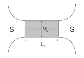
FIG. 1.: Schematic representation of a superconducting quantum point contact.

The general mean-field Hamiltonian for a superconducting system can be written in terms of the electron field operators $\hat{\psi}_{\sigma}(\vec{r})$

$$\hat{H}=\int d\vec{r}\;\left\{\sum_{\sigma}\hat{\psi}^{\dagger}_{\sigma}(\vec{r}){\cal H}_{e}(\vec{r})\hat{\psi}_{\sigma}(\vec{r})+\Delta^{*}(\vec{r})\hat{\psi}^{\dagger}_{\uparrow}(\vec{r})\hat{\psi}^{\dagger}_{\downarrow}(\vec{r})+\Delta(\vec{r})\hat{\psi}_{\downarrow}(\vec{r})\hat{\psi}_{\uparrow}(\vec{r})\right\}$$ (1)

where ${\cal H}_{e}$ is the one-electron Hamiltonian and $\Delta(\vec{r})$ is the superconducting order parameter. The problem of calculating transport properties in such a continuous representation for a non-homogenuous system is extremely involved requiring the knowledge of the adequate boundary conditions at the interfaces. Some attempts in this direction have been recently presented by Zaitsev and Averin [12] within the quasiclasssical Green functions approach. A different approach which circumvent these difficulties while keeping a fully microscopic description of the problem can be obtained by expanding the field operators in a discrete basis and writing the Hamiltonian (1) in the form [14]

$$\hat{H}=\sum_{i,\sigma}(\epsilon_{i}-\mu_{i})c^{\dagger}_{i\sigma}c_{i\sigma}+\sum_{i\neq j,\sigma}t_{ij}c^{\dagger}_{i\sigma}c_{j\sigma}+\sum_{i}(\Delta^{*}_{i}c^{\dagger}_{i\downarrow}c^{\dagger}_{i\uparrow}+\Delta_{i}c_{i\uparrow}c_{i\downarrow}),$$ (2)

where $i,j$ run over the different sites of the system, $t_{ij}$ are the hopping parameters connecting the different sites; $\mu_{i}$ and $\Delta_{i}$ being the chemical potential and order parameter in a site representation. The simplification introduced by this approach allows to deal with rather involved situations including spatial inhomogeneities (self-consistency) and non-stationary effects typically appearing in superconductors. For the voltage range $eV\sim\Delta$ the energy dependence of the transmission coefficients can be neglected and the transport properties can be expressed as a superposition of independent channels [13]. One can simplify even further the model to represent an SQPC with a single conduction channel, which can be described by the following Hamiltonian

$$\hat{H}=\hat{H}_{L}+\hat{H}_{R}+\sum_{\sigma}(te^{i\phi(\tau)/2}c^{\dagger}_{L\sigma}c_{R\sigma}+t^{*}e^{-i\phi(\tau)/2}c^{\dagger}_{R\sigma}c_{L\sigma})-\mu_{L}\hat{N}_{L}-\mu_{R}\hat{N}_{R},$$ (3)

where $H_{L,R}$ are the BCS Hamiltonians for the left and right uncoupled electrodes characterized by a constant order parameters $\Delta_{L,R}$ (for a symmetric contact $\Delta_{L}=\Delta_{R}=\Delta$). $\phi(\tau)$ is the time-dependent superconducting phase difference entering as a phase factor in the hopping terms describing electron transfer between the electrodes. In our model the transmission, $\alpha$, can be varied between 0 and 1 as a function of the coupling parameter $t$ (see [8] for details). Within this model, the total current through the contact can be written as

$$I(\tau)=\frac{ie}{\hbar}\sum_{\sigma}\left(te^{i\phi(\tau)/2}<c^{\dagger}_{L\sigma}(\tau)c_{R\sigma}(\tau)>-\;t^{*}e^{-i\phi(\tau)/2}<c^{\dagger}_{R\sigma}(\tau)c_{L\sigma}(\tau)>\right).$$ (4)

The averaged quantities appearing in the current can be expressed in terms of non-equilibrium Green functions [15]. For the description of the superconducting state it is useful to introduce spinor field operators (Nambu representation) [16], which in a site representation are defined as

$$\hat{\psi_{i}}=\left(\begin{array}[]{c}c_{i\uparrow}\\ c^{\dagger}_{i\downarrow}\end{array}\right)\hbox{ , }\hat{\psi}^{\dagger}_{i}=\left(\begin{array}[]{cc}c^{\dagger}_{i\uparrow}&c_{i\downarrow}\end{array}\right).$$ (5)

Then, the different correlation functions appearing in the Keldysh formalism adopt the standard causal form

$$\hat{G}_{ij}^{\alpha,\beta}(\tau_{\alpha},\tau^{\prime}_{\beta})=-i<\hat{T}[\hat{\psi}_{i}(\tau_{\alpha})\hat{\psi}_{i}^{\dagger}(\tau^{\prime}_{\beta})]>$$ (6)

where $\hat{T}$ is the chronological ordering operator along the closed time loop contour [15]. The labels $\alpha$ and $\beta$ refer to the upper ($\alpha\equiv+$) and lower ($\alpha\equiv-$) branches on this contour. The functions $\hat{G}^{+-}_{ij}$, which can be associated within this formalism with the electronic non-equilibrium distribution functions [17], are given by the (2x2) matrix

$$\hat{G}^{+-}_{i,j}(\tau,\tau^{\prime})=i\left(\begin{array}[]{cc}<c^{\dagger}_{j\uparrow}(\tau^{\prime})c_{i\uparrow}(\tau)>&<c_{j\downarrow}(\tau^{\prime})c_{i\uparrow}(\tau)>\\ <c^{\dagger}_{j\uparrow}(\tau^{\prime})c^{\dagger}_{i\downarrow}(\tau)>&<c_{j\downarrow}(\tau^{\prime})c^{\dagger}_{i\downarrow}(\tau)>\end{array}\right).$$ (7)

In terms of the $\hat{G}^{+-}$ the current is given by

$$I(\tau)=\frac{e}{\hbar}\;Tr\left[\hat{\sigma}_{z}\left(\hat{t}\hat{G}^{+-}_{RL}(\tau,\tau)-\hat{t}^{\dagger}\hat{G}^{+-}_{LR}(\tau,\tau)\right)\right],$$ (8)

where $\hat{t}$ is the hopping element in the Nambu representation

$$\hat{t}=\left(\begin{array}[]{cc}t&0\\ 0&-t^{*}\end{array}\right).$$ (9)

The Green functions $\hat{G}^{+-}_{ij}$ are calculated using an infinite order perturbation theory with the coupling term in Eq. (3) considered as a perturbation. Within this approach these Green functions obey a set of integral Dyson equations [8]. As discussed in the next sections, the solution is strongly dependent on the biasing condition which determines the time dependence in the superconducting phase difference.

III Current in a voltage biased contact

The simplest biasing condition is that of a constant applied voltage. This situation is rather easy to achieve experimentally except for very small voltages (see section IV). In spite of its apparent simplicity the theoretical analysis is quite complex because of the time-dependent phase-difference which gives rise to a time dependent current containing all harmonics of the Josephson frequency $\omega_{0}=2eV/\hbar$, i.e $I(\tau)=\sum_{n}I_{n}(V)\exp{in\omega_{0}}$. The current can be also decomposed into dissipative and nondissipative parts according to the different symmetry with respect to $V$ of even and odd terms in the previous expansion [8].

In this case the integral Dyson equations can be transformed into a set of algebraic equations by a double Fourier transformation, defined by

$$\hat{G}_{n,m}(\omega)=\int d\tau\int d\tau^{\prime}e^{-i\omega_{0}(n\tau-m\tau^{\prime})/2}e^{i\omega(\tau-\tau^{\prime})}\hat{G}(\tau,\tau^{\prime})$$ (10)

An efficient algorithm for the numerical evaluation of the Green function Fourier components is discussed in Ref. [8].

We shall concentrate in this section in the dc component of the current $I_{0}$ which is the quantity more readily accessible experimentally. Fig. 2 shows the dc $IV$ characteristics calculated from the fully quantum mechanical theory and from the semiclassical OBTK theory [18]. As can be observed the results become increasingly different for decreasing transmission. The fully quantum-mechanical calculation exhibits a pronounced subgap structure with steps at $eV=2\Delta/n$ which is hardly noticeable in the semiclassical theory. Both theories give the same result nevertheless for perfect transmission where interference effects, not included in the semiclassical theory, disappear due to the absence of backscattering.

The experimental $IV$ characteristics for atomic contacts of different metals are in remarkable agreement with our theoretical results. This is illustrated in Fig. 3 for the case of a one-atom contact made of Pb (these results are taken from Ref. [6]). This agreement has allowed to extract information on the conduction channels transmissions $T_{n}$ of metallic atomic contacts [5, 6, 19].

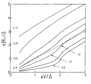
FIG. 2.: dc current-voltage characteristics of a SQPC for different values of the normal transmission. Left panel corresponds to the semiclassical OTBK theory and right panel to the fully quantum mechanical calculation.

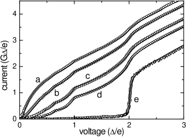
FIG. 3.: Measured current-voltage characteristics (symbols) for different realizations of a Pb one-atom contact at 1.5 K fabricated with the STM technique [6]. The full lines are numerical fits obtained by superposing four one-channel $IV$ curves with different transmissions.

The temperature dependence of the $IV$ characteristics is shown in Fig. 4 for different values of the transmission. A remarkable feature of this dependence is that the SGS persists up to temperatures close to the critical temperature. When normalized to the temperature dependent superconducting gap the dc current exhibits a certain increase at low transmission, the opposite behavior being found close to prefect transmission. The crossover between these two tendencies is found for $\alpha\sim 0.8$.

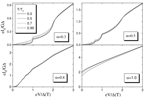
FIG. 4.: dc current-voltage characteristic for different temperatures and four values of the transmission.

The limit of very small bias is particularly interesting due to the contribution of MAR processes of increasing order $n\sim 2\Delta/eV$. This divergency in the $V\rightarrow 0$ limit is eventually controlled by the presence of an inelastic relaxation rate $\eta$ (usually a small fraction of the gap parameter) which introduces a cut-off in the theory when $eV<\eta$. The effect of the inelastic relaxation rate is to damp MAR processes of order $n>2\Delta/\eta$. As a consequence the system experiments a transition into a different regime where the total current becomes linear in $V$. In this regime the system response is determined by the adiabatic dynamics of the Andreev states at $\epsilon(\phi)=\Delta\sqrt{1-T\sin^{2}(\phi/2)}$ which move following the actual value of the superconducting phase. The total current can then be written as $I(\phi,V)=I_{S}(\phi)+G(\phi)V$ [20], where the supercurrent $I_{S}(\phi)$ and the phase-dependent linear conductance $G(\phi)$ are given by

$$I_{S}(\phi) = \frac{e\Delta}{2\hbar}\frac{\alpha\sin\phi}{\sqrt{1-\alpha\sin^{2}(\phi/2)}}\tanh(\frac{\beta\epsilon(\phi)}{2})$$ (11)

$$G(\phi) = \frac{2e^{2}}{h}\frac{\pi}{16\eta}\left[\frac{\Delta\alpha\sin\phi}{\sqrt{1-\alpha\sin^{2}(\phi/2)}}\mbox{sech}(\frac{\beta\epsilon(\phi)}{2})\right]^{2}\beta V.$$ (12)

The expression of the supercurrent [14, 21, 22] in Eq. (11) interpolates between the Josephson $I_{S}\sim\sin{\phi}$ behavior and the Kulik-Omelyanchuk $I_{S}\sim\sin{\phi/2}$ ballistic limit [23]. This behavior at high transmission has been recently confirmed experimentally using break junction techniques in an SQUID configuration [11]. It should be noticed that the expression of $G(\phi)$ gives a definite answer to an old-standing problem concerning the form of this term known as the “$cos{\phi}$ problem” [24]. The precise form of this term remains to be explored experimentally (a similar set up to that used in Ref. [11] could be used for this purpose).

Finally, it should be stressed that from a mathematically point of view the two limits $\eta\rightarrow 0$ and $V\rightarrow 0$ are not interchangeable [8]. In practice the limit $eV\rightarrow 0$ with $eV>\eta$ can never be reached as there is always a finite although small inelastic relaxation rate present.

IV Current biased contact

At very low voltages (and specially for high transmission) the contact impedance may become actually smaller than the voltage source impedance. If these conditions apply, the assumption of having an ideal source providing a constant voltage bias which fixes the phase dynamics is no longer valid. In this case one should take into account the electromagnetic environment of the contact in order to determine the phase dynamics and the system response to the external bias.

For conventional tunnel junctions this limit is usually analyzed by means of the RSJ and RSCJ models [2, 24] which represent the actual environment by a simple shunted circuit with a resistance $R$ and a capacitance $C$ connected in parallel to the junction. Within these simple models the phase dynamics is equivalent to that of a particle moving in a “tilted washboard” potential $U(\phi)=-I_{b}\phi+I_{c}\cos{\phi}$, where $I_{b}$ is the biasing current and $I_{c}$ is the Josephson critical current. At finite temperatures one should also consider thermal fluctuations acting as an stochastic force on the fictitious particle.

To analyze the response of an SQPC under current bias one should generalize these models for contacts of arbitrary transmission [25]. The description of the superconducting phase as classical variable will be valid as long as the Josephson coupling energy $E_{J}\sim\hbar I_{c}/2e$ is much larger than the charging energy $E_{C}\sim e^{2}/2C$. For an SQPC connected to a current source, the equations for the generalized RSCJ model would be given by

$$I_{b} = \frac{\hbar}{2e}C\ddot{\phi}+\frac{\hbar}{2e}G(\phi)\dot{\phi}+I_{S}(\phi)+i_{n}(\phi)$$ (13)

$$V = \frac{\hbar}{2e}\dot{\phi}$$ (14)

where $I_{S}(\phi)$ and $G(\phi)$ are given by Eq. (11) of the previous section and $i_{n}(\phi)$ is a fluctuating current whose power spectrum $S$ is related to $G(\phi)$ by the fluctuation-dissipation theorem $S=4k_{B}TG$ (see section VI). It should be noticed that the above equations are strictly valid in the limit of small voltages induced on the contact, i.e. $eV<\eta$, which is the condition for the validity of Eq. (11) in section III. The actual value of $\eta$ is unknown but can be estimated to be of the order of $\Delta/100$ or less [26]. In the mechanical analogy, the effective potential for the generalized RSCJ model can be written as

$$U(\phi)=-\left\{I_{b}\phi+\frac{4e}{\beta\hbar}\log\left[\mbox{cosh}\left(\frac{\beta\epsilon(\phi)}{2}\right)\right]\right\}$$ (15)

and there appears a “position” dependent friction which comes from the dissipative term in $G(\phi)$. The inclusion of this phase-dependent term should have important consequences in the dynamics of the system. Notice that the particular form of $G(\phi)$ (Eq. 11) introduces a very asymmetrical friction with a minimum at the local minima of $U(\phi)$ and maximum at the local maxima.

Integrating the Eqs. (12) of the generalized RSCJ model for arbitrary conditions is a formidable task. An approximate solution for the overdamped case, i.e. $G(\phi)/C>(2eI_{c}/\hbar C)^{1/2}$, can be obtained following the procedure introduced by Ambegaokar and Halperin [27] for overdamped tunnel junctions. The generalization of the Ambegaokar and Halperin theory is straightforward once we have identified the generalized potential (Eq. (13)) and the shunted resistance with $1/G(\phi)$ (details will be given elsewhere). The measurement of the slope of the $IV$ curve at zero voltage, which is directly related to $G(\phi)$, would provide information on the value of $\eta$ in real systems.

V Contact under microwave radiation

As discussed in section III, the Andreev states play a central role in determining the adiabatic dynamics of an SQPC at low bias voltage. Considering that typical subgap energies are in the microwave range, it seems natural to propose using microwave radiation for a direct detection of Andreev states. This possibility has been suggested in a previous work by us [28] and in Ref. [29].

The effect of a microwave external field can be easily introduced in the single channel contact model. One can assume that the field intensity is maximum in the constriction region and neglect the effect of field penetrating inside the electrodes. Within this assumptions the field can be introduced as a phase factor modulating the hopping term $t$ in Eq. (3), i.e.

$$t(\tau)=te^{i\alpha_{0}\cos{\omega_{r}\tau}},$$ (16)

where $\omega_{r}$ is the microwave frequency, $\alpha_{0}=eV_{opt}/(\hbar\omega_{r})$, $V_{opt}$ being the optical voltage induced by the field across the constriction. The parameter $\alpha_{0}$ measures the strength of the coupling with the external field. The time-dependent hopping term can be expanded as

$$t(\tau)=t\sum_{n}i^{n}J_{n}(\alpha_{0})e^{in\omega_{r}\tau},$$ (17)

where $J_{n}$ is the $n$-order Bessel function. For small coupling one can keep the lowest order terms in Eq. (15) and obtain some analytical results [28]. In the general case, the model Hamiltonian can be viewed, according to Eq. (15), as a superposition of processes where an arbitrary number of quanta of energy $\hbar\omega_{r}$ are absorbed or emitted. As the temporal dependence of each term in Eq. (15) is formally equivalent to that in the constant voltage case, the generalization of the algorithm discussed in section III to the present case is straightforward.

FIG. 5.: Induced dc current in a SQPC under microwave-radiation for different values of the transmission. The parameter $\alpha_{0}$ controls the coupling to the external field (see text).

Fig. 5 shows the induced dc current as a function of the microwave frequency for the case of low coupling constant ($\alpha_{0}=0.1$). All these results correspond to the situation in which the contact is carrying the maximum supercurrent. In this weak coupling limit the induced current is mainly due to the excitation from the lower to the upper Andreev state, which carries a negative current (i.e. opposite to the supercurrent). As a consequence the induced current exhibits a maximum for the resonant condition $\omega_{r}=2\epsilon(\phi)$. At resonance, the induced current can be of the same order as the critical supercurrent. One can also notice a second stellite peak around $\epsilon(\phi)$ associated with two photon processes and a continuous band above $\Delta+\epsilon(\phi)$. When the coupling constant $\alpha_{0}$ increases the contribution of higher order processes becomes progresively more important giving rise to a complex structure where the resonant condition for the excitation of the upper Andreev state can no longer be resolved [28].

VI Thermal and shot noise

The analysis of current fluctuations has a central role in the theory of transport in mesoscopic systems [30]. Fluctuations can provide useful information on the microscopic dynamics (correlations) not contained in the average current. It is thus desirable to develop a fully quantum mechanical theory of current fluctuations in an SQPC on an equal footing as previously discussed for the current. In this respect, some limiting cases have already been analyzed in the recent literature: the excess noise for $eV\gg\Delta$ in a ballistic contact has been discussed in Ref. [31], thermal noise for arbitrary transmission was analyzed in Ref. [32] while the case of perfect transmission and finite voltages has been addressed in Ref. [33].

The noise power spectrum is defined by

$$S(\omega,\tau)=\hbar\int d\tau^{\prime}\;e^{iw\tau^{\prime}}<\delta\hat{I}(\tau+\tau^{\prime})\delta\hat{I}(\tau)+\delta\hat{I}(\tau)\delta\hat{I}(\tau+\tau^{\prime})>$$ (18)

where $\delta\hat{I}(\tau)=\hat{I}(\tau)-<\hat{I}(\tau)>$. For the evaluation of the above correlation functions a BCS mean field decoupling procedure can be performed. $S(\omega,\tau)$ can then be written in terms of nonequilibrium Green functions introduced in section III. In the voltage biased case, $S(\omega,\tau)$ can be expanded in harmonics of the Josephson frequency, i.e. $S(\omega,\tau)=\sum S_{n}(\omega)\exp{in\omega_{0}\tau}$. As in the case of the average current the noise Fourier components $S_{n}(\omega)$ can be evaluated in terms of the Green functions matrix elements $G_{n,m}$ defined in section III.

Let us start by analyzing the $V=0$ case where noise is due to thermal fluctuations. While in a normal QPC thermal noise has the usual well understood behavior, increasing linearly with temperature and with a flat frequency spectrum, in the superconducting case it exhibits very unusual behavior as a function of temperature, frequency and phase. Fig. 6 illustrates the frequency dependence of the thermal noise for different transmissions. As can be observed the noise exhibits two sharp resonances at $\omega=0$ and $\omega=2\epsilon(\phi)$ corresponding to the excitation of the Andreev bound states. For $\omega>\Delta+|\epsilon(\phi)|$, $S$ exhibits a broad band arising from the continuous part of the single particle spectral density.

FIG. 6.: Power spectrum $S(\omega)$ of the zero-voltage current-fluctuations at $k_{B}T=0.2\Delta$ in a SQPC for three transmission values. The contact is biased at the maximum supercurrent.

The weight of the peaks at $0$ and $2\epsilon(\phi)$ can be evaluated analytically as discussed in Ref. [32]. We find that the zero frequency noise is related to the phase-dependent linear conductance by $S(0)=4k_{B}TG(\phi)$ as expected from the fluctuation dissipation theorem. The exponential temperature dependence in $G(\phi)$ gives rise to an exponential increase of thermal noise when $k_{B}T\sim\epsilon(\phi)$. It should be noticed that the ratio $S(0)/2eI_{S}(\phi)$ can actually be divergent for any temperature provided that $\alpha\rightarrow 1$ and $\phi\rightarrow\pi$. On the other hand, the weight of the peak at $2\epsilon(\phi)$ is zero for perfect transmission, increasing as $\alpha^{2}(1-\alpha)$, becoming the dominant feature for finite $1-\alpha$ and sufficiently low temperatures. In fact, the ratio between $S(2\epsilon(\phi))$ and $S(0)$ is given by

$$S(2\epsilon(\phi))/S(0)=\frac{1}{2}(1-\alpha)\tan^{2}{\frac{\phi}{2}}\mbox{cosh}\left[\frac{\epsilon(\phi)}{k_{B}T}\right].$$ (19)

Another quantity which is interesting to analyze and is directly amenable to experimental measurement is the shot-noise. Mathematically the shot-noise is given by the zero frequency dc component in the expansion of the noise power spectrum, i.e $S_{0}(0)$, at $eV\gg k_{B}T$. For simplicity we will consider the zero temperature case. Results for the shot-noise as a function of voltage are shown in Fig. 7 for several transmissions. The curves exhibit a pronounced subgap structure at the voltage values $eV=2\Delta/n$ as in the dc current. In the case of the shot-noise the structure is more pronounced and is still observable for transmissions rather close to 1. In the perfect ballistic limit shot-noise is greatly reduced due to correlations associated with the Pauli principle as in the case of a normal ballistic contact [34].

On the other hand, in the tunnel limit the shot-noise is expected to reach the Poisson limit $S\sim 2qI$, where $q$ is the transmitted charge in an elementary process. This relation offers the possibility to directly check whether multiple charges $q=ne$ are actually being transmitted coherently in a n-th order MAR process [35]. Our theory allows to calculate the effective charges defined by the shot-noise current ratio. In the tunnel limit one finds that $q$ exhibits a well defined step like behavior $q/e=1+Int[2\Delta/eV]$ confirming the above hypothesis [36].

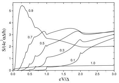
FIG. 7.: Zero-frequency current-fluctuations at zero temperature (shot-noise) as a function of bias voltage.

VII SGS and resonant tunneling

The model discussed so far describes an SQPC with an energy independent transmission $\alpha$. In some situations, that can be achieved experimentally, the normal transmission can have a non-negligible variation on an energy scale of the order of $\Delta$. This can happen when the constriction region is weakly coupled to the electrodes by tunnel barriers as in the case of a small metallic particle or a quantum dot coupled to superconducting leads [37]. We represent this situation by the following model Hamiltonian

$$\hat{H}=\hat{H}_{L}+\hat{H}_{R}+\sum_{\nu,\sigma}t_{\nu}(\hat{c}^{\dagger}_{\nu\sigma}\hat{c}_{0\sigma}+\hat{c}^{\dagger}_{0\sigma}\hat{c}_{\nu\sigma})+\sum_{\sigma}\epsilon_{0}\hat{n}_{0\sigma}+U\hat{n}_{0\uparrow}\hat{n}_{0\downarrow}$$ (20)

where $\hat{H}_{L}$ and $\hat{H}_{R}$ describe the left and right leads, $\epsilon_{0}$ is a resonant level associated with the isolated constriction region, $t_{\nu}$ with $\nu=L,R$ are hopping parameters which connect the level to the left and right leads. The $U$ term takes into account the Coulomb repulsion in the constriction region. The parameter $U$ is basically the charging energy, $E_{C}$, and is related to the central region capacitance $C$, by $U\sim e^{2}/2C$. For the subsequent discussion it is convenient to introduce the normal elastic tunneling rates $\Gamma_{\nu}=\pi|t_{\nu}|^{2}\rho_{\nu}(\mu)$, where $\rho_{\nu}(\mu)$ are the normal spectral densities of the leads at the Fermi level.

When the charging energy is much larger than both $\Gamma$ and $\Delta$ Andreev reflections are completely suppressed and transport is only due to single-quasiparticle tunneling. This situation has been achieved in experiments on transport through nanometer metallic particles by Ralph et al. [37]. Model calculations presented by us in Ref. [38] based on Hamiltonian (18) yield good agreement with the experimental results.

We shall consider in more detail the case of small charging energy, in which the interplay between resonant tunneling and MAR give rise to novel effects and a very rich subgap structure [38, 39]. Fig. 8 shows the dc $IV$ characteristic for different positions of the resonant level $\epsilon_{0}$ with respect to the Fermi level. The tunneling rates are taken in this case as $\Gamma_{L}=\Gamma_{R}=\Delta$. As can be observed, when the level is far from the gap region (case a) the limit of energy independent transmission is recovered and the subgap structure is similar to the one depicted in Fig. 2 (right panel). As the resonant level approaches the gap region the subgap structure becomes progressively distorted with respect to the energy independent transmission case. While the structure corresponding to the opening of odd-order MAR processes (i.e. at $eV\sim 2\Delta/n$ with odd $n$) is enhanced, the structure at $eV\sim 2\Delta/n$ with even $n$ is suppressed. When $\Gamma\rightarrow 0$ (not shown), one can also notice the appearance of resonant peaks in the $IV$ characteristic for $eV\sim 2\epsilon_{0}$.

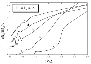
FIG. 8.: dc current-voltage characteristic for a resonant level $\epsilon_{0}$ coupled to superconducting leads. $\epsilon_{0}=5\Delta$ (a), $2\Delta$ (b), $\Delta$ (c), $\Delta/2$ (d) and 0 (e). $R_{N}(0)$ is the normal resistance at the Fermi level. Curves (c), (d) and (e) have been displaced for the sake of clarity.

VIII conclusions

An overview of the results of a microscopic theory for the transport properties of superconducting quantum point contacts has been presented. These results include the response under different biasing conditions for an energy independent transmission as well as the case of resonant transmission. A remarkable agreement has been found between the calculated and the experimental dc $IV$ curves for atomic-size contacts [5, 6]. The agreement has allowed to extract information on the number and transmissions of the conduction channels in atomic-contacts of different metallic elements [6, 19]. On the other hand, the agreement shows the importance of interference effects included in a fully quantum-mechanical calculation and thus the need to go beyond semiclassical theories for describing this kind of systems. Additional predictions of the microscopic theory remain to be analyzed experimentally. For instance, we could point out the phase dependence of the linear conductance, the direct observation of Andreev levels in contacts under microwave radiation and the analysis of shot-noise. This last analysis would provide direct evidence of coherent transmission of multiple charges in MAR processes. Finally, the rich SGS in the presence of resonant transmission could be explored in S-2DEG-S devices wich are currently being developed [3].

- [1] B.D. Josephson, Phys. Lett. 1, 251 (1962).
- [2] M. Tinkham, Introduction to Superconductivity, McGraw-Hill, New York (1996).
- [3] H. Takayanagi, T. Akazaki and J. Nitta, Phys. Rev. Lett. 75, 3533 (1995).
- [4] N. van der Post et al., Phys. Rev. Lett. 73, 2611 (1994).
- [5] E. Scheer et al., Phys. Rev. Lett. 78, 3535 (1997).
- [6] E. Scheer et al., Nature 394, 154 (1998).
- [7] D. Averin and A. Bardas, Phys. Rev. Lett. 75, 1831 (1995).
- [8] J.C. Cuevas, A. Martin-Rodero and A. Levy Yeyati, Phys. Rev. B 54, 7366 (1996).
- [9] M. Hurd, S. Datta and P.F. Bagwell, Phys. Rev. B 54, 6557 (1996).
- [10] E.N. Bratus et al., Phys. Rev. B 55, 1266 (1997).
- [11] M.C. Koops et al., G.V. van Duyneveldt and R. de Bruyn Ouboter, Phys. Rev. Lett. 77, 2524 (1996).
- [12] A.V. Zaitsev D.V. Averin, Phys. Rev. Lett. 80, 3602 (1998).
- [13] C.J.W. Beenakker, Phys. Rev. B 46, 12841 (1992).
- [14] A. Martin-Rodero, F.J. Garcia-Vidal and A. Levy Yeyati, Phys. Rev. Lett. 72, 554 (1994); Surf. Sci. 307-309 , 973 (1994); A. Levy Yeyati, A. Martin-Rodero and F.J. Garcia-Vidal, Phys. Rev. B 51, 3743 (1995).
- [15] L.V. Keldish, Zh. Eksp. Teor. Fiz. 47, 1515 (1964)[Sov. Phys. JETP 20, 1018 (1965).
- [16] Y. Nambu, Phys. Rev. 117, 648 (1960).
- [17] L.P. Kadanoff and G. Baym, Quantum Statistical Mechanics (Benjamin, New York, 1962).
- [18] T.M. Klapwijk, G.E. Blonder and M. Tinkham, Physica B 109-110, 1657 (1982); M. Octavio, M. Tinkham, G.E. Blonder and T.M. Klapwijk, Phys. Rev. B 27, 6739 (1983). K. Flensberg, J.B. Hansen and M. Octavio, Phys. Rev. B 38, 8707 (1988).
- [19] J.C. Cuevas, A. Levy Yeyati and A. Martin-Rodero, Phys. Rev. Lett. 80, 1066 (1998).
- [20] A. Martin-Rodero, A. Levy Yeyati and J.C. Cuevas, Physica B 218, 126 (1996); A. Levy Yeyati, A. Martin-Rodero and J.C. Cuevas, J. Phys.: Condens. Matter 8, 449 (1996).
- [21] W. Haberkorn, H. Knauer, and J. Richter, Phys. Status Solidi 47, K161 (1978).
- [22] C.W.J. Beenakker, Phys. Rev. Lett. 67, 3836 (1991).
- [23] O. Kulik and N. Omel’yanchuk, Fiz. Nizk. Temp. 3, 945 (1977); 4, 296 (1978) [Sov. J. Low Temp. Phys. 3, 459 (1997); 4, 142 (1978)].
- [24] A. Barone and G. Paterno, Physics and Applications of the Josephson Effect (Wiley, New York, 1982).
- [25] The case of perfect transmission has been recently discussed in D.V. Averin, A. Bardas and H.T. Iman, Phys. Rev. B 58 11165 (1998).
- [26] This small value is consistent with the agreement between theory and experiments in the constant voltage case.
- [27] V. Ambagaokar and B.J. Halperin, Phys. Rev. Lett. 22, 1364 (1969).
- [28] A. Levy Yeyati, J.C. Cuevas and A. Martin-Rodero, in Photons and Local Probes, edited by O. Marti and R. Müller (Kluwer Academic, Dordrecht, 1995).
- [29] V.S. Shumeiko, G. Wendin and E.N. Bratus, Phys. Rev. B 48, 13129 (1993).
- [30] For a recent review, see M.J.M. de Jong and C.W.J. Beenakker, in: Mesoscopic Electron Transport, ed. by L.L. Sohn, L.P. Kouwenhoven, and G. Schön, NATO ASI Series E, Vol. 345 (Kluwer Academic Publishing, Dordrecht, 1997).
- [31] J.P. Hessling et al., Europhys. Lett. 34 , 49 (1996).
- [32] A. Martin-Rodero, A. Levy Yeyati and F.J. Garcia-Vidal, Phys. Rev. B 53, R8891 (1996).
- [33] D. V. Averin and H.T. Imam, Phys. Rev. Lett. 76, 3814 (1996).
- [34] V.A. Khlus, Sov. Phys. JETP 66, 1243 (1987).
- [35] P. Dieleman et al., Phys. Rev. Lett. 79, 3486 (1997).
- [36] J.C. Cuevas, A. Martin-Rodero and A. Levy Yeyati to be published.
- [37] D.C. Ralph et al., Phys. Rev. Lett. 74, 3241 (1995).
- [38] A. Levy Yeyati et al., Phys. Rev. B 55, R6137 (1997).
- [39] G. Johansson et al., Physica C 293, 77 (1997).