NBI-HE-98-28

SPhT-98/119

Hamiltonian Cycles on Random Eulerian Triangulations

E. Guitter 

CEA-Saclay, Service de Physique Théorique

F-91191 Gif-sur-Yvette Cedex, France

C. Kristjansen  and J.L. Nielsen 

The Niels Bohr Institute

Blegdamsvej 17, DK-2100 Copenhagen Ø, Denmark

Abstract

A random Eulerian triangulation is a random triangulation where an even number of triangles meet at any given vertex. We argue that the central charge increases by one if the fully packed $O(n)$ model is defined on a random Eulerian triangulation instead of an ordinary random triangulation. Considering the case $n\rightarrow 0$, this implies that the system of random Eulerian triangulations equipped with Hamiltonian cycles describes a $c=-1$ matter field coupled to 2D quantum gravity as opposed to the system of usual random triangulations equipped with Hamiltonian cycles which has $c=-2$. Hence, in this case one should see a change in the entropy exponent from the value $\gamma=-1$ to the irrational value $\gamma=\frac{-1-\sqrt{13}}{6}=-0.76759...$ when going from a usual random triangulation to an Eulerian one. A direct enumeration of configurations confirms this change in $\gamma$.

PACS codes: 05.20.y, 04.60.Nc, 02.10.Eb
Keywords: Hamiltonian cycle, self-avoiding walk, random Eulerian lattice, fully packed $O(n)$ model

1 Introduction

In order to describe the thermodynamic properties of geometrical objects like polymers and membranes, it is important to be able to enumerate the possible configurations of such objects. One class of problems concerns the folding of these objects. The simplest non trivial examples are the compact folding of a self-avoiding polymer, in connection with protein folding, and the folding onto itself of a phantom (non self-avoiding) polymerised membrane. Traditionally one has studied the folding statistics of self-avoiding polymers by embedding them on a regular two-dimensional lattice and identifying the possible folded states of the polymer with the Hamiltonian cycles on the lattice [1]. A Hamiltonian cycle is a closed curve which visits each vertex of the lattice once and only once. Similarly, to describe the possible folded states of a phantom polymerised membrane one can approximate the membrane by a regular two-dimensional lattice and identify the possible folded states of the membrane with those of the lattice. In order to facilitate our discussion, we shall restrict ourselves to considering three-coordinate or equivalently triangular lattices. The problem of counting the number of folded states of the regular, triangulated lattice has been proven to be equivalent to a certain three-colouring problem, namely the problem of colouring the links of the lattice with three different colours so that no two links which belong to the same triangle carry the same colour [2]. This three-colouring problem is a classical mathematical problem which was solved by Baxter in 1970 [3]. It can also be described as the problem of solving the fully packed $O(n)$ model for $n=2$ [3]. Similarly, the problem of counting the number of Hamiltonian cycles on a regular three-coordinate lattice is equivalent to solving the fully packed $O(n)$ model in the limit $n\rightarrow 0$. This model is critical and describes a conformal field theory with central charge $c=-1$ [4, 5].

However, the use of a regular lattice to describe folding problems is clearly limitative. For instance, most membranes in nature are fluid rather than polymerised, and their modelling requires a random lattice instead. Similarly, one might speculate if the complex dynamics of polymers does not call for a random lattice rather than a regular one. Making use of the so-called fully packed $O(n)$ models on a random lattice (cf. section 3) it is possible to generalise the above mentioned folding problems to a random lattice. There are, however, some subtleties involved in this process. This is because the full packing constraint is very sensitive to the local geometry of the lattice. For instance when one solves the Hamiltonian cycle problem on a random three-coordinate lattice one finds that $c=-2$ [6, 7, 8]. We will explain the reason for this difference between the regular and the random case and argue that if we restrict the class of random triangulations considered to so-called random Eulerian triangulations we will find again $c=-1$. By random Eulerian triangulations we mean random triangulations where each vertex is shared by an even number of triangles. Such triangulations also appear when we try to generalise the membrane folding problem to a random lattice. If we consider simply the fully packed $O(2)$ model on a random lattice we do not get a model describing the folding of a random triangulation. We do also not get a model that describes the generalisation of Baxter’s three-colouring problem to a random lattice. In order to have a model which describes the generalised three-colour problem one must consider a fully packed $O(2)$ model where the length of the loops (appearing in the graphical representation of the model, cf. section 2) is restricted to being even [9]. Still, on a random lattice the edge-three-colouring problem is not equivalent to the folding problem. In order to have a model which describes the folding problem one must consider the edge colouring problem on a random Eulerian triangulation [9, 10] or equivalently the fully packed $O(2)$ model on a random Eulerian triangulation (note that the condition of the loops of the $O(n)$ model having even length is automatically satisfied on an Eulerian triangulation). Eulerian triangulations can also be described as triangulations permitting a three-colouring of their vertices [10]. The folding problem on a random lattice can hence be viewed as a double three-colouring problem.

In section 2 and 3 we review the properties of the fully packed $O(n)$ model on a regular and on a random lattice respectively and argue that on a random lattice we should see a change in central charge for the fully packed model if we change the class of triangulations considered from ordinary random triangulations to random Eulerian triangulations. In section 4 we specialise to the case $n\rightarrow 0$ and show that Hamiltonian cycles on a random Eulerian triangulation should provide us with an explicit realisation of a random surface model with an irrational value of the entropy exponent, $\gamma$. Section 5 describes a numerical solution of the Hamiltonian cycle problem on a random Eulerian triangulation and section 6 contains the results – results which support our arguments. Finally, in section 7 we conclude and comment on the similarity between our Hamiltonian cycle problem and another combinatorial problem which has recently attracted a lot of attention, namely the Meander problem [11].

2 Dense versus full packing of the $O(n)$-model on a regular lattice

Let us first consider a regular three-coordinate lattice, the honeycomb lattice, and let us associate to each vertex, $i$, of the lattice a $n$-component spin vector $\vec{S}_{i}$ with $\vec{S}_{i}^{2}=n$. The $O(n)$-model partition function is then given by

$$Z(T)=\int\prod_{i}d\vec{S}_{i}\prod_{<k,l>}\left(1+\frac{1}{T}\,\vec{S}_{k}\cdot\vec{S}_{l}\right),$$ (2.1)

where $\prod_{<k,l>}$ is the product over nearest neighbour vertices [12]. Expanding the product and integrating over spin variables it can be seen that the only terms which survive are those to which one can associate a collection of closed, self-avoiding and non-intersecting loops living on the lattice and that the partition function can also be written as [12]

$$Z(T)=\sum_{\{\cal L\}}\left(\frac{1}{T}\right)^{V(\{{\cal L}\})}n^{\cal N(\{{\cal L}\})}\equiv\sum_{\{\cal L\}}Z_{\{\cal L\}}.$$ (2.2)

Here the sum is over all loop configurations $\{\cal L\}$ having the above mentioned properties, $V(\{\cal L\})$ is the total number of vertices visited by loops and ${\cal N}(\{{\cal L}\})$ is the number of loops in $\{{\cal L}\}$. The representation (2.2) makes it possible to extend the definition of the $O(n)$-model to non-integer and to negative values of $n$. It is well-known that for $n\in[-2,2]$ the $O(n)$-model has a second order phase transition at some critical point $T=T_{c}(n)$ [13]. The model is also critical for $T<T_{c}(n)$ [13] and in this region of the coupling constant space it is denoted as the densely packed loop model, the name referring to the fact that the average length of the loops diverges while the number of vertices not visited by a loop stays finite (but non zero). The densely packed loop model describes a conformal field theory with central charge, $c_{d}$, related to $n$ in the following way [14]

$$c_{d}=1-\frac{6\nu^{2}}{1-\nu},\hskip 19.91684ptn=2\cos(\nu\pi),\hskip 14.22636pt\nu\in[0,1].$$ (2.3)

If we set $T=0$ in (2.1) or (2.2) we obtain the fully packed loop model. In this case only configurations where all vertices are visited by a loop contribute to the partition function. The fully packed loop model has been shown to describe a conformal field theory with central charge, $c_{f}$ given by [4, 5]

$$c_{f}=c_{d}+1=2-\frac{6\nu^{2}}{1-\nu},\hskip 19.91684ptn=2\cos(\nu\pi),\hskip 14.22636pt\nu\in[0,1].$$ (2.4)

If we send $n$ to zero in the fully packed loop model only configurations with one single loop visiting all vertices exactly once survive. In this case our partition function thus counts the number of Hamiltonian cycles on the honeycomb lattice. According to (2.4) this statistical mechanical model has central charge $c_{f}=-1$. This $n\to 0$ limit corresponds in practice to keeping the linear term in $n$ of the partition function (2.2). For $n$ identically equal to zero, one has $c_{f}=c_{d}=0$.

An explanation of the difference in central charge between the densely packed and the fully packed $O(n)$ model on the honeycomb lattice was given by Blöte and Nienhuis [4]. The fully packed loop model can be viewed as a superposition of a densely packed loop model and a SOS-model with central charge $c=1$. The extra SOS degree of freedom is a height variable which emerges only in the case of full packing. This height variable, $h_{v}$, lives on the vertices $v$ of the dual triangular lattice. It takes integer values and is defined by the demand that for nearest neighbour vertices $v$ and $v^{\prime}$, $|h_{v}-h_{v^{\prime}}|=1$ if the link between $v$ and $v^{\prime}$ has its dual link occupied by a loop and $|h_{v}-h_{v^{\prime}}|=2$ if not [4]. These local rules fix the value of the height variable without ambiguity on the entire lattice, up to a global additive constant and a global reversal of all the signs of $(h_{v}-h_{v^{\prime}})$. We note that the assignment of height variables divides the vertices of the triangular lattice into three different sets in such a way that no two neighbouring vertices belong to the same set: if we denote the three sets as $S_{i}$, $i=1,2,3$ the vertices belonging to $S_{i}$ can be characterised by having $h_{v}=i$ (mod 3). Therefore, the possibility of constructing the SOS height variable without frustrations essentially relies on the fact that the triangular lattice is vertex-three-colourable, i.e. can be divided into three sub-lattices of different colour with any two adjacent sites in different sub-lattices. The SOS model defined here is equivalent to the zero-temperature anti-ferromagnetic Ising model on the triangular lattice [15] and has central charge $c=1$ [16]. A nice way to visualise the height variables $h_{v}$ is to mark only those links of the triangular lattice which have $|h_{v}-h_{v^{\prime}}|=1$. This leads to a picture of a 3D-piling of cubes, whose surface profile is precisely described by the heights $h_{v}$, see figure 1.

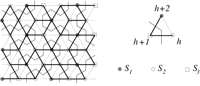
Figure 1: Construction of the SOS degree of freedom from the fully packed loops, on a regular triangular lattice. The thick lines indicate links whose dual link is occupied by a loop. The height variable $h$, defined on the vertices of the lattice, is such that the difference of height is $\pm 1$ for nearest neighbours connected by a thick line and $\pm 2$ for nearest neighbours connected by a dashed line. The sign is fixed by demanding that $h$ and the number $i$ of the corresponding sub-lattice $S_{i}$ are equal modulo 3. Viewing the thick line configurations as a 3D-piling of elementary cubes, the height variable corresponds precisely to the height of the surface of the piling.

3 Dense versus full packing of the $O(n)$-model on a random lattice

By duality we can view the $O(n)$-model on the honeycomb lattice as being defined on a regular triangulation and with that interpretation the model can be coupled to quantum gravity by the standard recipe. This leads to the so-called $O(n)$-model on a random lattice whose partition function reads [17]

$$Z(\lambda,T)=\sum_{\tau\sim S^{2}}e^{-\lambda N_{\tau}}\sum_{\{{\cal L}\}}\frac{1}{C_{\tau}(\{{\cal L}\})}Z_{\{{\cal L}\}}.$$ (3.1)

Here we sum over all triangulations, $\tau$ with the topology of the sphere $S^{2}$ and over all loop configurations $\{{\cal L}\}$ where it is understood that the loops live on the lattice dual to the triangulation. The quantity $C_{\tau}(\{{\cal L}\})$ is the order of the automorphism group of the triangulation $\tau$ with the loop configuration $\{{\cal L}\}$, $N_{\tau}$ is the number of triangles in the triangulation and $\lambda$ is the cosmological constant. Let us denote the triangles traversed by loops as decorated triangles and those not traversed by loops as non-decorated triangles. Then we can also write the partition function as

$$Z(\lambda,\kappa)=\sum_{\tau\sim S^{2}}e^{-\lambda N_{nd}}\sum_{\{{\cal L}\}}\frac{1}{C_{\tau}(\{{\cal L}\})}\,\kappa^{N_{d}}\,n^{{\cal N}(\{{\cal L}\})},\hskip 19.91684pt\kappa=e^{-\lambda}\,\frac{1}{T},$$ (3.2)

where $N_{nd}$ is the number of non-decorated triangles and $N_{d}$ is the number of decorated triangles. In the coupling constant space ($\lambda,\kappa$) of the model (3.2) there is a line of critical points beyond which the partition function does not exist. On this critical line there is a particular point $(\lambda^{*},\kappa^{*})$ where a phase transition takes place. This phase transition is the analogue of the phase transition at $T=T_{c}(n)$ seen on a regular lattice. For $\kappa<\kappa^{*}$ the singular behaviour of the partition function is due to the radius of convergence in $\lambda$ being reached while for $\kappa>\kappa^{*}$ the singular behaviour of the partition function is due to the radius of convergence in $\kappa$ being reached. If we approach the critical line from the region where $\kappa>\kappa^{*}$ we reach the densely packed loop model on a random lattice. This model has a scaling behaviour characteristic of a conformal matter field with central charge $c=c_{d}$ coupled to quantum gravity [17, 18].

If we set $e^{-\lambda}$ equal to zero while keeping $\kappa$ finite we obtain the fully packed loop model on a random lattice. This model has the same scaling behaviour as the densely packed model on a random lattice [17]. In particular, if we send $n\rightarrow 0$ in the fully packed model we get a model describing Hamiltonian cycles on a random three-coordinate lattice and this model has $c=-2$ [6, 7, 8].

The fact that one does not see any change in the central charge when going from the densely packed to the fully packed $O(n)$ model on a random lattice is not in contradiction with the above mentioned argument of Blöte and Nienhuis. As we already noticed, in order for the construction of the extra SOS degree of freedom to work it is necessary that the vertices of the triangular lattice can be divided into three sets so that no two neighbouring vertices belong to the same set. A necessary condition for this requirement to be fulfilled is that any vertex of the triangular lattice is shared by an even number of triangles. On a random lattice a vertex can be shared by any number of triangles so the condition is not met, thus preventing the construction of the SOS height variable.

The above requirement of vertex-three-colourability defines a particular class of triangulations which we shall call Eulerian triangulations. Such triangulations have been studied in [10], in connection with the problem of folding of random lattices. For triangulations with spherical topology, the three-colourability requirement and the constraint that any vertex is shared by an even number of triangles are actually equivalent [19]. The latter condition can be rephrased by demanding that the number of edges leaving any vertex is even, which is the well known property ensuring that the triangulation can be drawn in one path without lifting the pen, i.e. can be equipped with a Eulerian cycle passing each link once. An example of Eulerian triangulation is shown in figure 2.

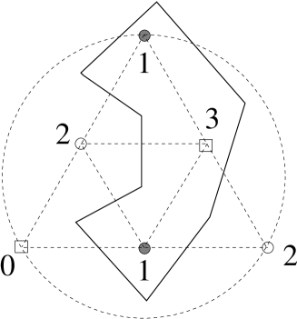
Figure 2: An Eulerian triangulation made of 8 triangles. Each vertex is shared by an even number of triangles. We have indicated the three subsets of different colours, as well as the height variables for a particular choice of Hamiltonian cycle (solid line).

If the argument of Blöte and Nienhuis is indeed correct we should be able to recover the shift by one in the central charge by restricting the fully packed model to Eulerian triangulations. Indeed, for an Eulerian triangulation of spherical topology equipped with a fully packed loop configuration, the construction of the SOS variable can be performed globally without frustration. In the case $n\rightarrow 0$ there is a particularly simple way of implementing this restriction to Eulerian triangulations, as discussed below.

4 Hamiltonian cycles on a random Eulerian triangulation

Let us consider the fully packed $O(n)$ model on a random Eulerian triangulation in the limit $n\rightarrow 0$. Its partition function reads (cf. equation (3.2))

$$Z(\kappa)=\sum_{N}\left(\sum_{(\tau_{E}\sim S^{2}(2N),{\cal H})}\frac{1}{C_{\tau_{E}}({\cal H})}\right)\kappa^{2N}\equiv\sum_{N}Z_{N}\,\kappa^{2N},$$ (4.1)

where the second sum is over random Eulerian triangulations of spherical topology, equipped with a Hamiltonian cycle, ${\cal H}$, and consisting of $2N$ triangles. Viewing these objects as two-dimensional quantum space-times decorated by configurations of some matter field, it follows from the work of David, Distler and Kawai [20] that $Z_{N}$ behaves as

$$Z_{N}\sim e^{\mu N}N^{\gamma-3}\left\{1+{\cal O}(\frac{1}{N})\right\},$$ (4.2)

where $\gamma$ is given by

$$\gamma=\frac{c-1-\sqrt{(25-c)(1-c)}}{12},$$ (4.3)

with $c$ being the central charge of the matter field. In the case of ordinary random triangulations equipped with Hamiltonian cycles one finds that the exponent $\gamma$ takes the value $\gamma=-1$ [6, 7, 8] which is characteristic of a matter field with $c=-2$. What we would like to show is that in the Eulerian case $\gamma$ takes the value characteristic of a matter field with $c=-1$, namely the irrational value

$$\gamma(c=-1)=\frac{-1-\sqrt{13}}{6}.$$ (4.4)

In order to do that we need to determine $Z_{N}$ in (4.1). Therefore, let us consider a random Eulerian triangulation of spherical topology equipped with a Hamiltonian cycle and consisting of $2N$ triangles. Since the triangulation is Eulerian, we can introduce a three-colouring of its vertices and this three-colouring of the vertices assigns to each triangle one of two possible orientations, $+$ and $-$. A triangle is said to have orientation $+$ if one encounters the colours of its vertices in the cyclic order 1-2-3 when moving counterclockwise along its edges. If the colours are encountered in the cyclic order 1-3-2 the triangle is said to have orientation $-$. Obviously, neighbouring triangles have opposite orientations and any Hamiltonian cycle drawn on the Eulerian triangulation visits alternatively $+$ and $-$ triangles.

We can now use a particular representation which facilitates our analysis. Let us represent the Hamiltonian cycle by a straight line having $2N$ vertices of alternating signs. The vertices represent the triangles visited by the loop and the signs the orientation of these triangles. As mentioned above, neighbouring triangles necessarily have opposite orientation. So far each triangle has only been given two neighbouring triangles. To completely specify a triangulation we must associate to each triangle one more neighbour. This can be done by connecting the vertices pairwise by arches. To ensure the planarity of the triangulation, vertices can only be connected either above or below the straight line representing the Hamiltonian cycle and different arches cannot intersect. Furthermore, an arch must always connect a $+$ to a $-$. This results in arch configurations of the type shown in figure 3.

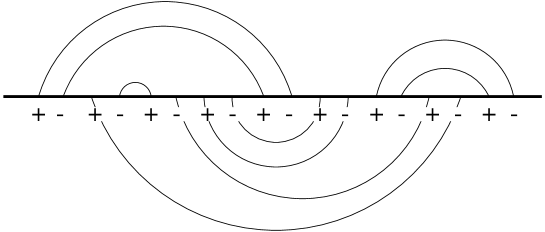
Figure 3: An arch configuration representing a planar Eulerian triangulation consisting of 18 triangles and being equipped with a Hamiltonian cycle. The $+$ and $-$ signs alternate along the straight line. Each arch connects a $+$ to a $-$.

Counting such arch configurations is equivalent to performing the second sum in equation (4.1). The symmetry factor is automatically taken into account. However, two arch configurations differing only by a cyclic permutation of vertices or by a reflection in the straight line represent the same triangulation. Hence, if we denote the total number of arch configurations involving $2N$ vertices as $M_{N}^{E}$ we have

$$M_{N}^{E}=2\times 2N\times Z_{N}\sim e^{\mu_{E}N}N^{\gamma_{E}-2}\left\{1+{\cal O}\left(\frac{1}{N}\right)\right\}.$$ (4.5)

We note that the problem of counting Hamiltonian cycles on an ordinary random lattice can likewise be reduced to a problem of counting arch configurations. The arch configurations appearing in that problem, however, are simpler than the present ones, having no signs associated with the vertices. The number of such configurations, $M_{N}$, can easily be counted using the Catalan numbers, $\{c_{N}\}$. One finds [7, 8]

$$M_{N}=c_{N}\,c_{N+1},$$ (4.6)

where

$$c_{N}=\frac{1}{N+1}\left(\begin{array}[]{c}\!2N\!\\ \!N\!\end{array}\right)\sim 4^{N}\,N^{-3/2}\hskip 8.5359pt\mbox{as}\hskip 8.5359ptN\rightarrow\infty,$$ (4.7)

leading to $\gamma-2=2\times(-3/2)$, hence $\gamma=-1$ as stated previously. In the present case where we expect to find an irrational value of $\gamma$ it is unlikely that a simple counting procedure can be found. In the next section we shall present some analytical considerations on the counting problem and describe a numerical solution.

5 Numerical solution

Our starting point is a vertex configuration of the type described above, i.e. a straight line with $2N$ vertices of alternating signs. We want to determine $M_{N}^{E}$, i.e. the number of ways of connecting pluses to minuses using two systems of non-intersecting arches, one drawn above the line and one drawn below the line. First, let us note that we have the obvious inequality $M_{N}^{E}\leq M_{N}$ from which we get the upper bound $\mu_{E}\leq\log(16)$ (cf. equations (4.6) and (4.7)). Next, let us derive a lower bound on $\mu_{E}$. For that purpose we consider the situation where all arches are drawn, say, above the line. In this case the requirement of non-intersection of the arches automatically leads to a configuration where pluses are connected to minuses since any arch must enclose an even number of vertices and hence connects a vertex at an odd position to a vertex at an even position. The number of such one-side non-intersecting arch configurations linking $2N$ points is exactly the $N$’th Catalan number, $c_{N}$. From a given one-side arch configuration we can construct a two-side arch configuration by flipping a number of arches to the other side of the line. The resulting arch configuration obviously contributes to $M_{N}^{E}$. Since there are $2^{N}$ ways of flipping $N$ arches, we immediately deduce that $M_{N}^{E}\geq 2^{N}c_{N}$ from which we obtain the lower bound $\mu_{E}\geq\log(8)$. Unfortunately, the flipping construction is not exhaustive since it produces only configurations where the upper and lower arches do not overlap, i.e. configurations where any vertex below a given, say, upper arch is connected to another vertex below the same arch even if the connection is made with a lower arch.

We shall describe below a systematic way of counting all the allowed configurations. First, let us note that $M_{N}^{E}$ can be written as

$$M_{N}^{E}=\sum_{k=0}^{N}C_{N,k}$$ (5.1)

where $C_{N,k}$ is the number of two-side arch configurations involving $2N$ vertices and having $k$, say, upper arches. We have the obvious symmetry

$$C_{N,k}=C_{N,N-k}.$$ (5.2)

It is possible to calculate $C_{N,k}$ explicitly for small values of $k$, as illustrated in Appendix A. For the first values of $k$, $C_{N,k}$ read explicitly:

$$C_{N,0} = c_{N},$$

$$C_{N,1} = N\,c_{N},$$

$$C_{N,2} = \frac{(2N-2)!}{(N-2)!(N+2)!}\left(3N^{3}-2N^{2}+4N\right),$$ (5.3)

$$C_{N,3} = \frac{(2N-3)!}{(N-2)!(N+3)!}\left(\frac{11}{3}N^{6}-15N^{5}+\frac{179}{3}N^{4}-117N^{3}+\frac{638}{3}N^{2}-192N\right)$$

$$-N\cdot 4^{N-2}.$$

Besides the trivial case $k=0$, the case $k=1$ can be easily understood by noticing that a two-side arch configuration with only one arch on top cannot have overlapping upper and lower arches. Therefore these arch configurations are exactly the arch configurations produced by starting from one of the $C_{N,0}=c_{N}$ arch configurations without arches on top and flipping one of its $N$ arches to the top. This simple procedure breaks down as soon as $k>1$ and one has to recourse to a more involved strategy described in Appendix A. As $k$ increases, however, one very soon runs into rather severe complications which limit the computation of explicit formulas to the very first values of $k$. In any case, for any finite $k$, one obtains the large $N$ scaling $C_{N,k}\sim 4^{N}$, far below the lower bound on $\mu_{E}$ and we expect that the main contribution to $M_{N}^{E}$ comes from terms $C_{N,k}$ with $k\approx N/2$. Unfortunately, it does not seem possible to calculate such terms analytically. We are not discouraged by this fact, however, because, as mentioned earlier, an irrational value of $\gamma$ is unlikely to be reproduced by a simple counting argument.

We shall now describe how one can calculate numerically $C_{N,k}$ for (in principle) any $N$ and $k$ using a recursive strategy. Again, let us start from a vertex configuration having $2N$ vertices of alternating signs and let us choose $k$ pluses and $k$ minuses which are to be connected above the straight line. The remaining $N-k$ pluses and $N-k$ minuses are then to be connected below the straight line. Instead of our original diagram we now have two sub-diagrams which are to be equipped by one-side arch configurations connecting pluses to minuses. Let us denote the number of ways of completing with arches a sub-diagram consisting of $k$ pluses and $k$ minuses as $c_{\sigma_{1}\sigma_{2}\ldots\sigma_{2k}}$ where $\sigma_{i}$ is $+1$ or $-1$ according to whether the vertex at position $i$ in the sub-diagram is a plus- or a minus-vertex. For $\sigma_{i}=(-1)^{i}$, $c_{\sigma_{1}\sigma_{2}\ldots\sigma_{2k}}$ is nothing but the $k$’th Catalan number, $c_{k}$. Obviously, $c_{\sigma_{1}\sigma_{2}\ldots\sigma_{2k}}$ is non zero if and only if the sequence of $\sigma_{i}$’s is globally neutral. There is no closed formula giving $c_{\sigma_{1}\sigma_{2}\ldots\sigma_{2k}}$ for an arbitrary sequence of $\sigma_{i}$’s. This is to be contrasted with the reverse problem, i.e. counting the number of $+/-$ sequences compatible with a given arch configuration, which is simply $2^{N}$ for $N$ arches since each arch must connect a plus at its left extremity to a minus at its right extremity or conversely. This implies in particular the following sum rule

$$\sum_{\{\sigma\}}c_{\sigma_{1}\sigma_{2}\ldots\sigma_{2N}}=\sum_{\rm arch\ configurations}2^{N}\,=\,2^{N}\,c_{N}.$$ (5.4)

Still, the $c_{\sigma_{1}\sigma_{2}\ldots\sigma_{2k}}$ fulfill a certain recursion relation which can easily be implemented in a computer program. To derive this recursion relation, let us consider a typical sub-diagram, such as the one depicted in figure 4.

Figure 4: An example of the decomposition of a sub-diagram.

In this diagram the first plus can be connected to any minus at an even position (if the plus is connected to a minus at an odd position it is impossible to complete the diagram without crossings). Placing the first arch divides the remaining vertices into two groups, those inside the arch and those to the right of the arch. These two groups of vertices can be considered separately since there can be no arches connecting them. This means that the $c_{\sigma_{1}\sigma_{2}\ldots\sigma_{2N}}$ fulfill the following recursion relation

$$c_{\sigma_{1}\sigma_{2}\ldots\sigma_{2N}}=\sum_{j=1}^{N}\delta_{\sigma_{1}+\sigma_{2j},0}\cdot c_{\sigma_{2}\ldots\sigma_{2j-1}}\cdot c_{\sigma_{2j+1}\ldots\sigma_{2N}},$$ (5.5)

where we have used the convention that $c_{\O}=1$. This recursion relation generalises the well known quadratic relation for Catalan numbers. To calculate $M_{N}^{E}$ numerically we now use the following obvious strategy

• Let $k$ run from $0$ to $\lfloor\frac{N}{2}\rfloor$, and for each $k$, select in all possible ways $k$ pluses and $k$ minuses to be connected above.

• Using the recursion relation compute the numbers of ways of completing the upper and lower sub-diagram that arise, and multiply these two numbers.

• Sum the results for all choices of sub-diagrams and all values of $k$.

• Multiply by 2. If $N$ is even, subtract the $k=\frac{N}{2}$-term once.

In practice, to make use of the recursion formula (5.5) we convert the string $\sigma_{1}\sigma_{2}\ldots\sigma_{2N}$ into a number ${\cal N}$ via the formula:

$${\cal N}=\sum_{i=1}^{2N}\left(\frac{\sigma_{i}+1}{2}\right)\cdot 2^{i-1},$$ (5.6)

and then save the number of ways of connecting the sub-diagram in a array under position ${\cal N}$. Our program pre-computes the number of connections for sub-diagrams up till ${\cal N}=2^{20}$ in order to save computer-time. Then formula (5.5) is only used, if a sub-diagram has a higher ${\cal N}$ than this, and such a sub-diagram is quickly reduced to diagrams having ${\cal N}$ less than $2^{20}$, where the pre-computed values can be used.

6 Results

In table 1 we list $M_{N}^{E}$ as a function of $N$ for $N=1,2,\ldots,20$ as determined by the computer algorithm described in the previous section. For comparison we list also the corresponding number, $M_{N}$, counting arch systems describing ordinary random triangulations equipped with Hamiltonian cycles (cf. equation (4.6)). Furthermore, in table 2 we list $C_{N,k}$ for $N\leq 12$ (cf. equation (5.1)). We note that in accordance with our expectations (cf. section 5) we observe that the main contribution to $M_{N}^{E}$ comes from the $C_{N,k}$’s with $k\approx\frac{N}{2}$. From the data for $M_{N}^{E}$ we shall seek to extract the quantities $\mu_{E}$ and $\gamma_{E}$ (cf. equation (4.5)) using a variant of a ratio method introduced in the study of random surface models in [21] (for a general discussion, see [22]). For a generic $M_{N}\sim e^{\mu N}N^{\gamma-2}\{1+{\cal O}(1/N)\}$, we have that

$$\mu_{N}^{(0)} \equiv \log\left(\frac{M_{N+1}}{M_{N}}\right)=\mu+{\cal O}\left(\frac{1}{N}\right),$$ (6.1)

$$\gamma_{N}^{(0)} \equiv 2-N^{2}\log\left(\frac{M_{N+2}M_{N}}{M_{N+1}^{2}}\right)=\gamma+{\cal O}\left(\frac{1}{N}\right).$$ (6.2)

From these series of estimates we can get improved series of estimates, for instance the series $\gamma_{N}^{(p)}$ given by

$$\gamma_{N}^{(p)}\equiv\frac{1}{p!}\sum_{i=0}^{p}(N+i)^{p}\left(\begin{array}[]{c}\!p\!\\ \!i\!\end{array}\right)\,(-1)^{p-i}\gamma_{N+i}^{(0)}=\gamma+{\cal O}(\frac{1}{N^{p+1}}),$$ (6.3)

and similarly for $\mu$.

$N$	$M_{N}^{E}$	$M_{N}$
1	2	2
2	8	10
3	40	70
4	228	588
5	1424	5544
6	9520	56628
7	67064	613470
8	492292	6952660
9	3735112	81662152
10	29114128	987369656
11	232077344	12228193432
12	1885195276	154532114800
13	15562235264	1986841476000
14	130263211680	25928281261800
15	1103650297320	342787130211150
16	9450760284100	4583937702039300
17	81696139565864	61923368957373000
18	712188311673280	844113292629453000
19	6255662512111248	11600528392993339800
20	55324571848957688	160599522947154548400

Table 1: The numbers $M_{N}^{E}$ (random Eulerian triangulations) and $M_{N}$ (ordinary random triangulations) for $N=1,$ 2, $\ldots,20$.

$\scriptstyle k\backslash N$	1	2	3	4	5	6	7	8	9	10	11	12
0	1	2	5	14	42	132	429	1430	4862	16796	58786	208012
1	1	4	15	56	210	792	3003	11440	43758	167960	646646	2496144
2		2	15	88	460	2250	10549	48048	214344	941460	4085950	17566032
3			5	56	460	3172	19551	111584	602514	3121020	15655970	76559920
4				14	210	2250	19551	147288	1002078	6320460	37614016	213817902
5					42	792	10549	111584	1002078	7978736	57977304	392238792
6						132	3003	48048	602514	6320460	57977304	479421672
7							429	11440	214344	3121020	37614016	392238792
8								1430	43578	941460	15655970	213817902
9									4862	167960	4085950	76559920
10										16796	646646	17566032
11											58786	2496144
12												208012

Table 2: The numbers $C_{N,k}$ for $N\leq 12$.

In figures 5 and 6, we plot $\mu_{N}^{(p)}$ and $\gamma_{N}^{(p)}$ as a function of $N$ for $p=2,3,4,5$ for the Hamiltonian cycles on the ordinary random triangulations (dashed lines) as well as for the Hamiltonian cycles on the random Eulerian triangulations (full lines). The series $\mu_{N}^{(p)}$ and $\gamma_{N}^{(p)}$ are expected to converge faster the larger the value of $p$. However, the larger $p$ the smaller the amount of data.

Figure 5: $\mu_{N}^{(p)}$ as a function of $N$ for $p=2$, 3, 4, 5 for Hamiltonian cycles on ordinary random triangulations (dashed lines) and on random Eulerian triangulations (full lines).

Figure 6: $\gamma_{N}^{(p)}$ as a function of $N$ for $p=2$, 3, 4, 5 for Hamiltonian cycles on ordinary random triangulations (dashed lines) and on random Eulerian triangulations (full lines).

In table 3 we list our final estimates for $\mu$ and $\gamma$ extracted from the series $\mu_{N}^{(p)}$ and $\gamma_{N}^{(p)}$ for ordinary random triangulations (RT) and random Eulerian triangulations (RET). We also give for comparison the exact result for ordinary random triangulations.

	$\mu$	$\gamma$
RT (exact)	$\log(16)\approx 2.772589$	$-1$
RT (estimated)	$2.772590\pm 10^{-6}$	$-1.000000\pm 10^{-6}$
RET	$2.313\pm 0.001$	$-0.76\pm 0.02$

Table 3: Final estimates for $\mu$ and $\gamma$ for Hamiltonian cycles on ordinary random triangulations (RT) and random Eulerian triangulation (RET) along with the exact results for the RT-case.

The ratio method reproduces neatly the exact values for the ordinary random triangulations. When we make the restriction to random Eulerian triangulations we clearly see a difference in the behaviour of $\mu_{N}^{(p)}$ and $\gamma_{N}^{(p)}$. In the case of $\mu_{N}^{(p)}$ the convergence is as rapid as for ordinary random triangulations but the asymptotic value is smaller. We note that our estimate $\mu_{E}\sim 2.313$ respects the bounds $\log(8)\leq\mu_{E}\leq\log(16)$ derived in section 5, as it should. In the case of $\gamma_{N}^{(p)}$ we observe an oscillatory behaviour, not present for the usual random triangulations. Since the amplitude of the oscillations decreases as $N$ increases the data still allows us to extract a reliable estimate for $\gamma$. This estimate for $\gamma$ agrees well with the predicted irrational value $\gamma_{E}=(-1-\sqrt{13})/6\approx-0.768$ and definitely differs from the value $\gamma=-1$ characteristic of Hamiltonian cycles on usual random triangulations.

7 Conclusion

We have argued that one should see an increase of the central charge by one unit when one considers the fully packed $O(n)$ model on a random Eulerian triangulation instead of an ordinary random triangulation. Our argument was based on an explanation of Blöte and Nienhuis why one sees an increase in central charge when moving from the densely packed to the fully packed $O(n)$ model on a regular lattice [4] (cf. section 2). We have tested our prediction by numerical analysis in the case $n\rightarrow 0$ which corresponds to Hamiltonian cycles on random Eulerian triangulations and on ordinary random triangulations respectively. Whereas the latter system has $c=-2$ the first one should according to our prediction have $c=-1$. Our numerical analysis confirms the prediction. In particular this means that we have found an explicit realisation of a random surface model with an irrational value of the entropy exponent, $\gamma$, not at any point evoking analytical continuation. In addition, our results support the explanation of Blöte and Nienhuis.

Let us denote by ${\cal M}_{N}(q)$ the number of Hamiltonian cycles on a lattice with $N$ sites and coordination number $q$. A mean field argument of H. Orland et al. [23] gives that

$$\omega_{H}=\lim_{N\rightarrow\infty}\frac{1}{N}\log{\cal M}_{N}(q)=\frac{q}{e}.$$ (7.1)

In the present case we find that the number of Hamiltonian cycles on random Eulerian triangulations behaves as $\left[\exp(2.313)\right]^{T/2}$ where $T$ is the number of triangles or equivalently the number of vertices on the dual lattice. The number of random Eulerian triangulations consisting of $T$ triangles, on the other hand, is known to behave as $\sqrt{8}^{T}$ [10]. This gives the following average value of $\omega_{H}$

$$\langle\omega_{H}\rangle\approx\left(\frac{e^{2.313}}{8}\right)^{1/2}=1.124,$$ (7.2)

which is very close to the mean field value $\frac{3}{e}\approx 1.104$. For the honeycomb lattice one has $\omega_{H}=\frac{3^{3/4}}{2}\approx 1.140$ [5].

It would be interesting to extend our analysis of the $O(n)$ model on random Eulerian triangulations to other values of $n$. The case $n=2$ is particularly interesting since, as explained in the introduction, this case describes the folding problem of a random triangulation onto itself, modelling a fluid membrane. As likewise explained in the introduction, this folding problem can be viewed as an edge-three-colouring problem on a random vertex-three-colourable triangulation. The system of vertex-three-colourable triangulations has been found to have central charge $c=0$ [10] and so has the edge three-colouring problem on a usual random triangulation [9]. Amazingly, when coupling these two models one should get a model with central charge $c=2$.

Figure 7: An example of a Meander configuration with $4$ connected components.

Finally, we would like to make a connection between our problem and another problem of arches, that of Meanders. Originally, the Meander problem consists in enumerating the number of pairs of arch systems connecting $2N$ points both from above and from below and such that the path resulting from connecting the upper and lower arches is made of a single connected component. This problem turns out to be equivalent to the compact folding onto itself of a closed linear self-avoiding polymer. By extension, one also considers the possibility of creating several connected components, with a weight $q$ per connected component. Figure 7 shows an example of a Meander configuration with $4$ connected components. The partition function one wants to evaluate is therefore

$$z_{N}(q)=\sum_{a,b}q^{c(a,b)},$$ (7.3)

where $a$ and $b$ are arbitrary systems of arches connecting $2N$ points on one side (say the upper side for $a$ and the lower side for $b$) of a straight line, and $c(a,b)$ is the number of connected components obtained by connecting these arches. As for our problem, one expects $z_{N}(q)\sim e^{\mu(q)N}N^{\gamma(q)-2}$ at large $N$. Except for the particular cases $q=1$, $q=-1$ and $q\to\infty$ which can be solved explicitly, only numerical estimates for $\mu$ and $\gamma$ are known. As for our system, the Meander problem is a problem of interacting arch systems. In our case, the interaction comes from the fact that the upper and lower arches have to connect pluses and minuses for two sub-sequences of the same alternating sequence. In the Meander problem, the interaction concerns the number of created connected components. It is interesting to note that this interaction can also be reformulated in terms of sequences of pluses and minuses to be connected by arches. Indeed, as shown in [11] (in a slightly different language), the quantity $q^{c(a,b)}$ can be written as

$$q^{c(a,b)}=\sum_{\{\sigma\}\ a\ {\rm and}\ b\atop\ \ {\rm connectable}}u^{\frac{1}{2}\left(P(a,\{\sigma\})+P(b,\{\sigma\})-Q(a,\{\sigma\})-Q(b,\{\sigma\}\right)},$$ (7.4)

for $q=u+1/u$ and where the sum is over all sets $\{\sigma\}$ of pluses and minuses which are such that both $a$ and $b$ connect only pluses to minuses (we say: $a$ and $b$ connectable). Here $P(a,\{\sigma\})$ (respectively $Q(a,\{\sigma\})$) denote the number of arches in $a$ connecting a plus (respectively a minus) at the left extremity of the arch to a minus (respectively a plus) at the right extremity. For $u=1$ for instance, this leads to

$$z_{N}(2)=\sum_{a,b}\sum_{\{\sigma\}\ a\ {\rm and}\ b\atop\ \ {\rm connectable}}1=\sum_{\{\sigma\}}c_{\sigma_{1}\sigma_{2}\cdots\sigma_{2N}}^{2},$$ (7.5)

to be compared with equation (5.4). We thus see here that one of the main difficulties in the Meander problem actually consists in the determination of the coefficients $c_{\sigma_{1}\cdots\sigma_{2N}}$ for arbitrary sequences. In this sense, solving our problem would be a first step in the solution to the Meander problem.

Acknowledgements     We thank J. Ambjørn, B. Durhuus and J. Jurkiewicz for useful discussions and O. Golinelli for a critical reading of the manuscript.

Appendix A

In this Appendix, we will explain how to compute the coefficients $C_{N,k}$ for the first values of $k$. Let us illustrate our strategy by calculating $C_{N,1}$ in a way which can be generalised to larger values of $k$. We again start from a vertex configuration involving $2N$ vertices of alternating signs. Now we must choose a plus and a minus which are to be connected above the line. There are two different situations that we need to consider. Either the plus chosen is situated to the left of the minus chosen or the plus chosen is situated to the right of the minus chosen. Corresponding to these two possibilities we write with an obvious notation

$$C_{N,1}=C_{N,1}^{+-}+C_{N,1}^{-+}.$$ (A.1)

Let us now consider the first situation (cf. figure 8).

Figure 8: Choosing one plus and one minus divides the diagram into three sub-diagrams.

By choosing the plus and the minus which are to be connected above the line we split the vertex configuration into three sub-configurations, I, II, and III. These three sub-configurations all contain an equal number of pluses and minuses and we shall denote such configurations as neutral. If we considered instead the opposite situation only the sub-diagram in the middle would be neutral. The left-most sub-diagram would have a plus in excess and the right-most sub-diagram would have a minus in excess. Such diagrams will be denoted as positively and negatively charged respectively. As we shall see later the charge of a sub-diagram plays an important role in the counting process. Now the vertices of the three sub-diagrams must be connected by arches drawn below the line. A vertex of sub-diagram II cannot be connected to a vertex of sub-diagram I or III. However, nothing prevents vertices from sub-diagram I from being connected to vertices of sub-diagram III and we can consider the union of these two sub-diagrams as one sub-diagram. In general a series of sub-diagrams can be connected if the resulting diagram is one with alternating signs. Now, we can immediately write down an expression for $C_{N,1}^{+-}$. Instead of calculating directly $C_{N,k}$, however, it proves convenient to calculate first the corresponding generating functional $C_{k}(z)=\sum_{N=0}^{\infty}C_{N,k}\,z^{N}$. Denoting the number of vertices in sub-diagram I as $2i$ and the number of vertices in sub-diagram II as $2j$ we have

$$C_{1}^{+-}(z) = \sum_{N=0}^{\infty}\sum_{i=0}^{N-1}\sum_{j=0}^{N-1-i}c_{j}\,c_{N-j-1}z^{N}=\sum_{N=0}^{\infty}\sum_{j=0}^{N-1}(N-j)c_{j}\,c_{N-j-1}z^{N}$$ (A.2)

$$= zC(z)\frac{d}{dz}\left(zC(z)\right),$$

where

$$C(z)=\sum_{N=0}^{\infty}c_{N}z^{N}=\frac{1-\sqrt{1-4z}}{2z}.$$ (A.3)

By similar considerations one finds for $C_{N,1}^{-+}(z)$

$$C_{1}^{-+}(z)=\sum_{N=0}^{\infty}\sum_{i=1}^{N-1}\sum_{j=0}^{N-1-i}c_{j}\,c_{N-j-1}z^{N}=zC(z)\left(z\frac{d}{dz}C(z)\right),$$ (A.4)

the difference from the previous case being the lower limit in the second sum (which is due to the fact that in this case sub-diagram I is positively charged). Thus, in total we get

$$C_{1}(z)=z\frac{d}{dz}\left(zC(z)^{2}\right),$$ (A.5)

which means that

$$C_{N,1}=N\,c_{N},$$ (A.6)

in agreement with equation (5.3). For $k=1$, the above calculation is clearly not the simplest way to reach the desired result, but it has the advantage that it can be generalised to the $C_{N,k}$’s with a finite $k>1$ even if, as we shall see, one very soon runs into a rather severe complication. Let us illustrate this by calculating $C_{2}^{+-+-}(z)$ In this case choosing the four vertices which are to be connected above the line divides the vertex configuration into five sub-diagrams I, II, III, IV and V which are all neutral (cf. figure 9).

Figure 9: Choosing two pluses and two minuses divides the diagram into five sub-diagrams.

It is not possible to connect a vertex of a sub-diagram with an odd number to a vertex of a sub-diagram with an even number, but all other combinations are allowed. For $C_{2}^{+-+-}(z)$ one thus has, cf. figure 9

$$C_{2}^{+-+-}(z)=2\sum_{N=0}^{\infty}\sum_{i=0}^{N-2}\sum_{j=0}^{N-2-i}\,\sum_{k=0}^{N-2-i-j}\,\,\sum_{l=0}^{N-2-i-j-k}\left\{c_{j+l}\,c_{k}\,c_{N-2-j-k-l}\right.$$ (A.7)

$$\hskip 28.45274pt\left.+c_{N-2-j-l}\,c_{j}\,c_{l}-c_{j}\,c_{k}\,c_{l}\,c_{N-2-j-k-l}\right\}z^{N}.$$

The first term in the sum represents the configurations where we allow (but not enforce) connections between region II and region IV and forbid connections between region III and region I or V, The second term represents the configurations where we forbid connections between regions II and IV, allowing connections between region III and the regions I and V. There is an overlap between the configurations which contribute to these two terms and to remove this overlap we must subtract exactly the third term, corresponding to situations where the regions II, III and IV are not connected to any other region. In the present case it is straightforward to remove the overlap but for higher values of $k$ the overlapping becomes a severe complication.

As long as one is able to keep track of the overlaps, however, there are simple diagrammatic rules by means of which $C_{k}(z)$ can be constructed. Let us assume that we are aiming at constructing $C_{k}^{\sigma_{1}\sigma_{2}\ldots\sigma_{2k}}(z)$ where $\sigma_{1}\sigma_{2}\ldots\sigma_{2k}$ is a given sequence of $k$ pluses and $k$ minuses. Choosing the $k$ pluses and the $k$ minuses which are to be connected above the line divides the original vertex configuration into $2k+1$ sub-configurations. To calculate $C_{k}^{\sigma_{1}\sigma_{2}\ldots\sigma_{2k}}(z)$ we must sum over all possible ways of connecting these sub-diagrams and if necessary subtract overlapping configurations. Assume that we have chosen one particular way of allowing connections between the $2k+1$ sub-diagrams. Our particular choice has arranged the sub-diagrams into groups $G_{i}$ of possibly connected diagrams. The contribution to $C_{k}^{\sigma_{1}\sigma_{2}\ldots\sigma_{2k}}(z)$ from this particular way of connecting the sub-diagrams can be written as

$$z^{k}c_{\sigma_{1}\sigma_{2}\ldots\sigma_{2k}}\prod_{i}F_{G_{i}}(z).$$ (A.8)

Here $c_{\sigma_{1}\sigma_{2}\ldots\sigma_{2k}}$ counts the number of ways of connecting the $k$ pluses and $k$ minuses above the line. If the total number of sub-diagrams in a group $G$ is denoted as $m$ and the number of positively charged sub-diagrams is denoted as $m_{+}$, it is easily shown that $F_{G}(z)$ takes the form

$$F_{G}(z)=\frac{1}{(m-1)!}z^{m_{+}}\frac{d^{m-1}}{dz^{m-1}}\left(z^{m-1-m_{+}}C(z)\right).$$ (A.9)

For instance in the case of $C_{N,2}^{+-+-}$ one finds immediately

$$C_{2}^{+-+-}(z)=2z^{2}C(z)\left[\frac{d}{dz}(zC(z))\right]^{2}+2z^{2}C(z)^{2}\frac{1}{2}\frac{d^{2}}{dz^{2}}(z^{2}C(z))-2z^{2}C(z)^{3}\frac{d}{dz}(zC(z)),$$

which is easily seen to coincide with the expression (A.7). Using the rules (A.8) and (A.9) as well as the explicit expression for $C(z)$ (cf. equation (A.3)) we have been able to determine $C_{N,2}$ and $C_{N,3}$, as given in equation (5.3). It is obvious that as long as we consider $k$ finite, $C_{k}(z)$ can be expressed in terms of a finite number of terms involving only the function $C(z)$ and its derivatives and thus $C_{N,k}\sim 4^{N}$ at large $N$.

References

- [1] M. Gordon, P. Kapadia and A. Malakis, J. Phys. A: Math. Gen. 9 (1976) 751; P.D. Gujrati, J. Phys. A: Math. Gen. 13 (1980) L437; T.G. Schmalz, G. E. Hite and D.J. Klein, J. Phys. A: Math. Gen. 17 (1984) 445; J. Suzuki and T. Izuyama, J. Phys. Soc. Jpn. 57 (1988) 818.
- [2] P. Di Francesco and E. Guitter, Europhys. Lett. 26 (1994) 455, cond-mat/9402058.
- [3] R.J. Baxter, J. Math. Phys. 11 (1970) 784.
- [4] H.W.J. Blöte and B. Nienhuis, Phys. Rev. Lett. 72 (1994) 1372.
- [5] M.T. Batchelor, J. Suzuki and C.M. Yung, Phys. Rev. Lett. 73 (1994) 2646, cond-mat/9408083.
- [6] B. Duplantier and I. Kostov, Nucl. Phys. B340 (1990) 491.
- [7] B. Eynard, E. Guitter and C. Kristjansen, Nucl. Phys. B528 [FS] (1998) 523, cond-mat/9801281.
- [8] S. Higuchi, Mod. Phys. Lett. A13 (1998) 727, cond-mat/9806349.
- [9] B. Eynard and C. Kristjansen, Nucl. Phys. B516 [FS] (1998) 529, cond-mat/9710199.
- [10] P. Di Francesco, B. Eynard and E. Guitter, Nucl. Phys. B516 [FS] (1998) 543, cond-mat/9711050.
- [11] P. Di Francesco, O. Golinelli and E. Guitter, Mathl. Comput. Modelling 26 (1997) 97, hep-th/9506030; Commun. Math. Phys. 186 (1997) 1 (where an equivalent form of Eq. (7.4) can be found), hep-th/9602025; Nucl. Phys. B482 [FS] (1996) 497, hep-th/9607039; Y. Makeenko and Yu. Chepelev, hep-th/9601139; P. Di Francesco, J. Math. Phys. 38 (1997) 5905, hep-th/9702181; Commun. Math. Phys. 191 (1998) 543, hep-th/9612026; M.G. Harris, hep-th/9807193.
- [12] E. Domany, D. Mukamel, B. Nienhuis and A. Schwimmer, Nucl. Phys. B190 [FS] (1981) 279.
- [13] B. Nienhuis, Phys. Rev. Lett. 49 (1982) 1062.
- [14] VI.S. Dotsenko and V.A. Fateev, Nucl. Phys. B240 [FS] (1984) 312.
- [15] H.W.J. Blöte and H.J. Hilhorst, J. Phys. A 15 (1982) L631.
- [16] H.W.J. Blöte and M.P. Nightingale, Phys. Rev. B47 (1993) 15046.
- [17] I. Kostov, Mod. Phys. Lett. A4 (1989) 217.
- [18] B. Duplantier and I. Kostov, Phys. Rev. Lett. 61 (1988) 143.
- [19] Mathematical Intelligencer Volume 19 Number 4 (1997) 48; Volume 20 Number 3 (1998) 29.
- [20] F. David, Mod. Phys. Lett. A3 (1988) 1651, J. Distler and H. Kawai, Nucl. Phys. B321 (1989) 509.
- [21] F. David, Nucl. Phys. B257 (1985) 543; J. Ambjørn, B. Durhuus, J. Frölich and P. Orland, Nucl. Phys. B270 (1986) 457; J. Ambjørn, B. Durhuus and J. Frölich, Nucl. Phys. B275 (1986) 161; F. David, J. Jurkiewicz, A. Krzywicki and B. Petersson, Nucl. Phys. B290 (1987) 218
- [22] D. Shanks, J. Math. Phys. XXXIV (1955) 1
- [23] H. Orland, C. Itzykson and C. de Dominicis, J. Phys. Lett. 46 (1985) L-353