Fun with Quantum Dots

Abstract

We consider quantum dots with a parabolic confining potential. The qualitative features of such mesoscopic systems as functions of the total number of electrons $N$ and their total angular momentum $J$, e.g. magic numbers, overall symmetries etc., are derived solely from combinatoric principles. The key is one simple hypothesis about such quantum dots yielding a basis of states (different from the usual single electron states one starts with) which is extremely easy to handle. Within this basis all qualitative features are already present without the need of any perturbation theory.

I Introduction

Quantum dots with a parabolically confined potential are a particularly simple species of a phenomenon enjoying increasing interest [1]. The basic novelty with such systems is their being mesoscopic, i.e. the fact that they live on the edge between classical and quantum physics. Quantum dots are sometimes called artificial atoms, which illuminates their mesoscopic nature. Indeed, although much larger than a real atom, the angular momentum $j$ of the electrons is quantized, and hence, via the classical relation $j\propto r^{2}$, its orbital radius.

It has been known for some time [2, 3] that the total potential energy of a (parabolic confining) quantum dot with $N$ electrons exhibits local minima for certain amounts of the total angular momentum $J$, called magic numbers. In fact, the local minima occur when

$$J(N,k)=\frac{N(N-1)}{2}+kN\,,\ \ \ \ k\in{{Z}}_{+}\,.$$ (1)

The quantum nature of the system becomes even more apparent when we compare the behaviour for $N\leq 5$ electrons with the one for $N\geq 6$ electrons. Classically, we expect that the lowest energy configuration for $N\leq 5$ electrons is a regular $N$-gon, while for $N\geq 6$ electrons it should be a regular $(N-1)$-gon with one electron in the center. However, whenever $k=(N-1)k^{\prime}$ with $k^{\prime}\in{{Z}}_{+}$, the configuration at such special magic numbers is much less symmetric than the classical counterpart. In fact, it behaves much more like a Laughlin-type quantum droplet.

We will demonstrate in this letter that the appearance of magic numbers as well as the loss of symmetry for the special magic numbers satisfying

$$J(N,k^{\prime}(N-1))=N(N-1)\left[k^{\prime}+\frac{1}{2}\right]\,,\ \ \ \ k^{\prime}\in{{Z}}_{+}\,,$$ (2)

can be explained by pure combinatorics. To do so, we need a bit of preparation.

We assume that the external magnetic field is strong enough to completely polarize all electrons. Then, only one electron can occupy an eigenstate of the angular momentum operator with eigenvalue $j\in{{Z}}_{+}$. The system characterized by the total number of electrons $N$ and the total angular momentum $J$ may now reside in any quantum mechanical state of the form $[j_{1},\ldots j_{N}]$ such that $0\leq j_{1}<j_{2}<\ldots<j_{N}$ and $\sum_{i=1}^{N}j_{i}=J$, where the $j_{i}$ denote the angular orbitals in which the electrons may stay. Of course, the $N$ electrons are identical particles meaning that each angular momentum eigenstate is a one-particle state antisymmetrized over all the electrons. To count the number of possible configurations one simply has to expand the combinatoric partition function

$$Z(y,q)=\prod_{n=0}^{\infty}(1+yq^{n})=\sum_{N,J}c_{N,J}y^{N}q^{J}\,.$$ (3)

The product includes the term $n=0$ since one electron may reside in the $j=0$ state. The reader might convince themselves that $c_{N,J}$ can be quite large even for very small electron numbers and medium sized total angular momenta. The true state is a complicated superposition of these configurations which depends on the precise interaction of the electrons giving each configuration a different weight. The problem is that each configuration is a sum of $N$ single-particle states. The latter are eigenstates only for the free Hamiltonian without interactions. At this point, numerical methods are usually employed to diagonalize the physical Hamiltonian which includes the Coulomb interaction as well as other effects [4].

Here, we will take a different approach. First, we note that any configuration $[j_{1},\ldots,j_{N}]$ might contain so-called blocks of adjacent angular orbitals which are all occupied. Such a block $j_{i},j_{i}+1,\ldots,j_{i}+n-1$ is uniquely characterized by two numbers, namely the number $n$ of adjacent occupied orbitals, and the number $\bar{\jmath}=(j_{i}+j_{i}+1+\ldots+j_{i}+n-1)/n=j_{i}+\frac{1}{2}(n-1)$. It is clear that we can enumerate all the configurations also by the blocks they decompose into, $[(n_{1},\bar{\jmath}_{1}),(n_{2},\bar{\jmath}_{2}),\ldots,(n_{\ell},\bar{\jmath}_{\ell})]$. Note that $\bar{\jmath}$ might be half-integer, and that $(1,\bar{\jmath})$ denotes an orbital which does not have an occupied neighbouring orbital. Of course, $1\leq\ell\leq N$ with the extreme cases given by either one complete block or only isolated single orbitals. Since the angular momentum orbital also defines a radial quantization, electrons in a block are also radially adjacent. In some abuse of language we might view each such configuration, projected on the radial component, as a configuration of a spin chain where spins can either be occupied or not. This leads us to the one hypothesis we will make in this paper:

Hypothesis: The electrons within a block $(n,\bar{\jmath})$ are (sufficiently strongly) coupled due to spin-spin and spin-orbit interactions to form a composite state of charge $n$ and “spin” $\bar{\jmath}$, while there is no (or negligible) spin-spin and spin-orbit interaction among different blocks.

Clearly, this hypothesis is the equivalent of a nearest-neighbour interaction approximation. The clue is that we can treat a block as a collective state. In particular, antisymmetrizing is performed seperately for each block, which will influence certain multiplicities. Also, the Coulomb interaction between two blocks $(n_{1},\bar{\jmath}_{1})$ and $(n_{2},\bar{\jmath}_{2})$ is calculated classicaly as given by the potential between two rings of charge $n_{1}$ and $n_{2}$ with radii $\sqrt{\bar{\jmath}_{1}}$ and $\sqrt{\bar{\jmath}_{2}}$ respectively. Here and in the following we adopt a system of units in which all proportionality constants are put to one, since we are only concerned with qualitative features. However, in most computations only ratios appear, making them independent of our particular choice of units. Our choice is motivated by keeping everything as close as possible to pure integers emphasizing the combinatorical nature of our approach.

Our basis of composite states does already account for spin-spin effects, the remaining other important effect being the Coulomb interaction. However, to further simplify all calculations, we make the following observation: It has been shown numerically that the qualitative behavior of classical dots is quite independent of the precise nature of the repulsive interaction $V({\rm\bf r}_{i},{\rm\bf r}_{j})=e_{i}e_{j}|{\rm\bf r}_{i}-{\rm\bf r}_{j}|^{-\gamma}$, with $\gamma=1$ yielding the Coulomb case, see e.g. [5]. The same should hold for quantum dots, as our results confirm a posteriori for $\gamma=2$. This is called universality, a property which quantum dots share with Laughlins wave functions for the fractional quantum Hall effect at filling factors $\nu=1/(2p+1)$. However, the formulæ for the potential energy between blocks and, in particular, the self-energy of a block, can only be given in a simple closed form in $n$ and $\bar{\jmath}$ for $\gamma$ even. Since the spirit of this paper is simplicity, we will therefore put $\gamma=2$ with the silent understanding of universality. We have checked for a wide range of $N,J$ that the qualitative features are indeed not affected by this.

Thus, within our setting, the self-energy of a block $(n,\bar{\jmath})$ is given, in the equilibrium state, by the potential energy of a regular $n$-gon of radius $\sqrt{\bar{\jmath}}$, which yields

$$E_{(n,\bar{\jmath})}=\frac{(n+1)n(n-1)}{3!\,4\bar{\jmath}}\,.$$ (4)

Similarly, the potential energy between two such blocks is simply

$$E_{(n_{1},\bar{\jmath}_{1}),(n_{2},\bar{\jmath}_{2})}=\frac{n_{1}n_{2}}{|\bar{\jmath}_{1}-\bar{\jmath}_{2}|}\,.$$ (5)

Note that the squared radii in these formulæ have been replaced by the “spins” of the composite states, bringing everything down to rational numbers. It will be imporant later that, if we were to include the precise proportionality factor of the relation $j=m_{e}\omega r^{2}$, it would yield a common factor to all these partial energies. We are now ready to proceed in finding magic numbers.

II Magic Numbers

All we have to do is calculate the energies for all block configurations according to the above formulæ, where we neglect any pure quantum mechanical effects (such as the rest energy $\frac{1}{2}N\hbar$) as well as the kinetic term (which is linear in $J$) yielding the so-called excitation energy

$$E_{m} \equiv E[(n_{1},\bar{\jmath}_{1}),\ldots,(n_{\ell},\bar{\jmath}_{\ell})]$$ (6)

$$= \sum_{i=1}^{\ell}E_{(n_{i},\bar{\jmath}_{i})}+\sum_{i<k}E_{(n_{i},\bar{\jmath}_{i}),(n_{k},\bar{\jmath}_{k})}\,,$$ (7)

where we have assumed that we have enumerated all configurations (in a completely arbitrary manner) by $m$. We will now assume that the normalized ground state of the quantum dot can be written as a linear combination $|{\Psi}\rangle=\sum_{m}S_{m}\exp(-\frac{1}{2}\beta E_{m})|{\Psi_{m}}\rangle$, with the $|{\Psi_{m}}\rangle$ forming an ortho-normal system, i.e. each configuration $m$ will be weighted accordingly by its Boltzman factor $\exp(-\beta E_{m})$. The inverse temperature $\beta$ is as yet unknown, but can easily be determined by solving the normalization condition

$${\cal Z}(\beta)=\sum_{m}S_{m}\exp(-\beta E_{m})=1\,.$$ (8)

Please note that this is much easier than it looks! Putting $x=\exp(-\beta)$, one only has to find the unique real zero of the polynomial ${\cal Z}(x^{\prime})-1$ which lies in the interval $x^{\prime}\in[0,1]$. Here $x^{\prime}=x^{1/M}$ with $M$ the least common multiple of all denominators of the rational(!) numbers $E_{m}$, and the polynomial ${\cal Z}(x^{\prime})-1\in{{Z}}[x^{\prime}]$. Finding this one zero can be done to arbitrary percision and very quickly, even for huge polynomials. The $S_{m}$ are symmetry factors which take into account that each block is antisymmetrized individually, but also that each block $(n,\bar{\jmath})$ has a discrete ${{Z}}_{n}$ symmetry. Hence individual antisymmetrization yields for each such block a symmetry factor $n!|{{Z}}_{n}|^{-1}=(n-1)!$. This has to be multiplied by the number of ways to distribute the $N$ electrons among the $\ell$ blocks of a given configuration. Hence

$$S_{m}\equiv S[(n_{1},\bar{\jmath}_{1}),\ldots,(n_{\ell},\bar{\jmath}_{\ell})]={N\choose\ell}\prod_{i=1}^{\ell}(n_{i}-1)!\,,$$ (9)

such that the probability of the $m$-th configuration is $p_{m}=S_{m}\exp(-\beta E_{m})$.

Alternatively, we could leave $\beta$ undetermined, treating it as an outer parameter of the system. This amounts in allowing different values for the normalization constant ${\cal Z}(\beta)$. Again, we have checked that the qualitative features vary weakly with $\beta$. Fixing $\beta$ as above yields – in a loose sense – the quantum mechanical (inverse) temperature, a measure of how likely the system fluctuates

FIG. 1.: Thermodynamic data for a parabolic confining quantum dot with $N=5$ electrons and total angular momentum $10\leq J\leq 60$. The magic numbers at which the energy as well as the temperature exhibit local minima can clearly be seen. At these numbers, the entropy also has local minima indicating that the system has higher order for these angular momenta. Indeed, the system is closest to a cristalline structure at the magic numbers. The behaviour of the entropy is contrasted with the logarithm of the number of configurations.

quantum mechanically between its different states (neglecting thermal fluctuations due to a heat bath).

After determining $\beta$, we have the complete partition function of our quantum dot system which we now treat as a system in statistical mechanics. Therefore we can easily determine observables such as the energy $\langle{E}\rangle=\partial_{\beta}\log({\cal Z})=\sum_{m}p_{m}E_{m}$, the specific heat $\langle{C}\rangle\equiv\beta^{-2}C_{v}=\partial_{\beta}^{2}\log({\cal Z})=\langle{E^{2}}\rangle-\langle{E}\rangle^{2}$, and the entropy $S=-\sum_{m}p_{m}\log(p_{m})$. As figures 1 and 2 demonstrate, the magic numbers show up in these observables exactly as they are supposed to do. We compare the most interesting cases, $N=5$ and $N=6$. The temperature $1/\beta$ and the specific heat are multiplied by suitable factors to improve their appearance in the plots. It should be noted that all these calculations, whose results are collected in the plots, only take a few minutes with a small and simple C-program on a typical workstation.

Naturally, the “smoothness” of the curves shown in figures 1 and 2 increases with $N$ and for each $N$ with $J$ due to the fast growth of $c_{N,J}$. However, we find it noteworthy that a mesoscopic system of only 2 or 3 particles already shows the same features, i.e. can successfully be approximated by a statistical system. One can interpret this fact that quantum mechanics in a mesoscopic system shows itself mainly by moving the sys-

FIG. 2.: Thermodynamic data for a parabolic confining quantum dot with $N=6$ electrons and total angular momentum $15\leq J\leq 75$. Compare the magic numbers with the ones for $N=5$. A close look reveals that in addition to the period $N=6$ of magic numbers, equation (1), another period of $N-1=5$ is superimposed according to [3] which coincides with the former for $J=45$. Of course, the same is true for the $N=5$ quantum dot, but less prominently expressed. Note that magic numbers can already be seen for very small $J\sim J_{{\rm min}}=N(N-1)/2$.

tem from a purely classical configuration to a statistical one. To show more clearly what we mean by this, we will consider the radial probability distribution, i.e. $p(R)_{N,J}=\int_{0}^{2\pi}|\Psi(R,\phi)_{N,J}|^{2}\,{\rm d}\phi$ for given $N,J$. The point is that we do not even have to calculate anything of the wavefunction $\Psi(R,\phi)_{N,J}$. Since angular momentum and orbital radius are interlinked, we only need to consider the formal sum

$$\tilde{R}(q)=\sum_{m}p_{m}\sum_{i=1}^{\ell_{m}}\frac{n_{i}}{N}q^{\bar{\jmath}_{i}}=\sum_{j=0}^{J}\tilde{p}_{j}q^{j}\,,$$ (10)

where again $m$ stands for the $m$-th configuration of blocks $[(n_{1},\bar{\jmath}_{1}),\ldots,(n_{\ell},\bar{\jmath}_{\ell_{m}})]$. The mathematically inclined reader may wish to consider this as some kind of discrete Fourier transform of the radial or, more precisely, angular momentum probability distribution. The radial distribution can then be read off as $p(R=\sqrt{j})=\tilde{p}_{j}$. However, we assumed here that the composite block state $(n,\bar{\jmath})$ is localised at $\bar{\jmath}$. Since this state is a collective state out of $n$ electrons occupying the orbits from $\bar{\jmath}-\frac{n-1}{2}$ to $\bar{\jmath}+\frac{n-1}{2}$, it will certainly be smeared out over this region in angular momentum space. In the spirit of treating the system as a statistical mechanics ensemble, the most natural distribution of the composite state is a binominal distribution centered at $\bar{\jmath}$ with width $\frac{n}{2}$. One could equally take the point of view that a Gaussian distribution is more natural for a quantum mechanical state. However, since we are only interested in a qualitative analysis, we may neglect the difference between these two distributions (one may convince onself that both distributions lead to very similar functions $p(r)$). Since $\bar{\jmath}$ may be half integer, the correct binominal distribution yields

$$\hat{R}(q) = \sum_{m}p_{m}\sum_{i=1}^{\ell_{m}}\frac{n_{i}}{N}\sum_{l_{i}=0}^{2n_{i}-2}{2n_{i}-2\choose l_{i}}\frac{q^{\bar{\jmath}_{i}+\frac{1}{2}(l_{i}+1-n_{i})}}{2^{2n-2}}$$ (11)

$$= \sum_{j=0}^{J}\hat{p}_{j}q^{j}$$ (12)

as the radial distribution function. We are now ready to discuss the issue of symmetry loss, which is observed at the special magic numbers eq. (2) for $N\geq 6$.

III Symmetry Loss

The smallest non-trivial special magic number for $N=5$ is $J(5,4)=30$, and for $N=6$ it is $J(6,5)=45$. Direct numerical analysis shows that around these numbers, $(N-1)$-gon symmetry with an occupied center is the preferred symmetry, whereas at the precise special magic numbers, and $N\geq 6$, symmetry is even more weakly expressed. One speaks of a fluid-like state at these numbers (in analogy to Laughlins quantum droplets), and says that the quantum dot with these particular values of total angular momentum $J=(N,k^{\prime}(N-1))$ has filling factor

$$\nu=\frac{1}{2}\frac{N(N-1)}{J}=\frac{\frac{1}{2}N(N-1)}{N(N-1)(k^{\prime}+\frac{1}{2})}=\frac{1}{2k^{\prime}+1}\,.$$ (13)

Before studying the radial distributions, we would like to explain this fact, and also that it is only observed for $N>5$. For smaller particle numbers, ${{Z}}_{N}$ symmetry is not broken (or only very slightly). Our considerations are made from very simple general assumptions and do not rely on any numerical studies. The key ingredient is the following relation between different magic numbers:

$$J(N,(N-1)k^{\prime})=$$ (15)

$$J(L,(L-1)k^{\prime})+J(N-L,(N+L-1)k^{\prime}+L)\,.$$

Note that this relation can be applied recursively! The meaning is that for the special magic numbers, there are several ways to build a state out of smaller magic units. However, the above relation is quite different from the trivial relation $J(N,k)=J(L,k)+J(N-L,k+L)$, which just divides one block of angular momentum eigenstates into two adjacent ones. The former relation is to be understood as follows. If the offset $k$ is divisible by $N-1$ and sufficient large, ${{Z}}_{N}$ symmetry can be replaced by ${{Z}}_{L}$ symmetry (with a rather small offset) within ${{Z}}_{N-L}$ symmetry (with an even larger offset). This is possible, because this distribution of angular momenta among the particles gives the same magic number, but with two sufficiently separated blocks to allow separate antisymmetrization.

Clearly, this alone does not force loss of symmetry. The question is, which of these possible distributions has the lowest energy, and how close do the energies of the other distributions come to the minimal one. To answer these questions, one only needs the formulæ (4), (5), and (6), and compare energies of different configurations. If the system were classical, we would only have to compare $E[(N,J/N)]$ with $E[(N-1,J/(N-1)),(1,0)]$. The former energy is smaller than the latter as long as $N<\frac{1}{4}(13+\sqrt{73})<6$. Since a quantum dot is quantum mechanical by definition, all possible configurations contribute and we have to calculate the full partition function ${\cal Z}$ instead.

The above formula (15) is recursive. Moreover, one of the magic numbers on the right hand side is again a special magic number. Thus, it appears that the fluid-like quantum state is due to the fact that (for “large” $N$) there are a lot of different antisymmetrizations possible at these numbers which – as we are going to show – have all comparable similar energies, where the energy of the center occupied $(N-1)$-gon configuration is the minimal one for $N>5$. There even exist antisymmetrizations with three or more nested blocks, whenever $N$ is large enough.

We can read off the loss of symmetry from the radial distribution function. At a magic number $J$, we would expect it to have a well defined peak centered at $R=\sqrt{J}$ for $N\leq 5$, and for $N\geq 6$ it should show two equally high peaks, one at $R=0$. However, we find something quite different from that. In the following plot (figure 3), we compare the radial distributions for a range $39\leq J\leq 51$ around the special magical value $J=45$ for $N=6$. One clearly sees that at the ordinary magic numbers $J=39,51$ full ${{Z}}_{6}$ symmetry is restored (since there is no peak at $R=0$)! ${{Z}}_{5}$ symmetry with one particle in the center is most prominently exhibited for the neighbouring values $J=40,50$. This very sensitive dependency on the value of $J$ is a pure quantum effect contradicting classical expectations. However, the behaviour at the special magic number $J=45$ is different. There is a certain probability for a particle to sit in the center, but it is only half of the probability of the main peak. This tells us that the main peak cannot come alone from the configuration with a five particle block and one particle in the center.

One way to interpret this result is to say that a quantum dot behaves either more as a quantum mechanically system or more as a statistial ensemble depending on the value of the filling factor $\nu$ defined in (13). The system is very much like a statistical ensemble and most resembles

FIG. 3.: Some radial distributions for a quantum dot with $N=6$ electrons and total angular momentum $39\leq J\leq 51$. Magic numbers are $J=39,45,51$ with $J=45$ being a special magic number. Note that the classically expected 5-fold symmetry is only observed for $J=J_{{\rm mag}}\pm 1$. This is because the system prefers forming composite states which works best for magic numbers. However, the neighbouring $J$-values behave similar to atoms with one shell either almost filled or filled plus one excess electron.

a quantum droplet for $\nu=\frac{1}{2k^{\prime}+1}$ with $k^{\prime}\in{{Z}}_{+}$ which precisely happens for $J$ being a special magic number. That is the same condition as for the filling factor for Laughlin-type fractional quantum Hall states which are described via the one-component plasma analogy as statistical systems! The system is very quantum mechanical, and in fact resembles most an atom-like structure, when $J$ is a non-special magic number. This does not translate into a straightforward statement with respect to the filling factor.

The best way to compare the behavior at special magic numbers (2) with the one at ordinary magic numbers (1) would be to calculate the 2-point charge density correlation $p({\rm\bf r},{\rm\bf r}_{0})$. In numerical studies of quantum dots, one usually freezes the position of one electron at ${\rm\bf r}_{0}$ and computes the probability of finding a charge at ${\rm\bf r}$. If ${\rm\bf r}_{0}$ is chosen such that it lies in an angular momentum orbital of high probability, one will get plots which clearly exhibit the symmetry properties of the quantum dot state. However, to do this we would need the wave function which we avoided calculating. But the information encoded in (11) is sufficient to give us a semi-classical approximation of the charge distribution. We simply pick the configuration with the lowest energy and put us into its “rest frame”. By this we mean the following: The minimal energy configuration has a certain block decomposition, and for this

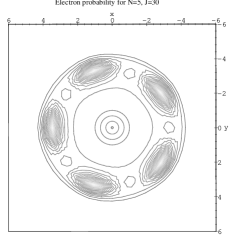
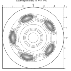
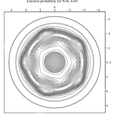
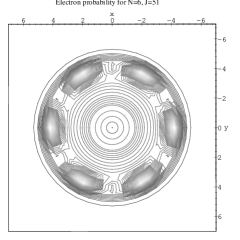
FIG. 4.: Comparsion of approximated charge distributions (in the rest frame of the minimal energy configuration) for $N=5$ (top) and $N=6$ (bottom). Left are special magic numbers corresponding to $\nu=1/3$, right are ordinary magic numbers. Note the difference for $N=5$ and $N=6$, the latter showing much stronger quantum droplet behavior at a special magic number.

decomposition we localize the electrons on the edges of the appropriate $n$-gons, smeared out according to the binominal distribution taking into account the quantum mechanical width of the $n$-gons. For $N\leq 5$ the minimal configuration is simply one $N$-gon, for $6\leq N\leq 8$ it is a $(N-1)$-gon with an occupied center. For $N\geq 9$ we have a shell like structure where the relative orientation of the electrons in one shell to the ones in another would have to be chosen according to the classical solution. All other configurations are considered to be radially symmetric. In this way, superimposing these approximations of charge distributions, we obtain a measure of how much the minimal energy configuration sticks out of the other ones, and hence a measure of how much the particular symmetry of the minimal energy configurations determines the symmetry of the full charge distribution. When plotting charge distributions in this manner, it is clear that the integrated radial probability for a block within a configuration (first equation in 11) has to be weighted not only by the binominal distribution, but also by $1/2\pi r$ where the radius $r$ varies over the width where the block is localized. Moreover, such a charge distribution is naturally time averaged. To be more precise, we approximate the probability distributions as follows: A block $(n,\bar{\jmath})$ with probability $p$, if it does not have the dominant symmetry of the minimal energy configuration, contributes

$$\tilde{p}(j,\phi)=p\,{\cal D}_{n/2}(j-\bar{\jmath})\frac{1}{2\pi\sqrt{j+1}}\,,$$ (16)

where ${\cal D}_{\sigma}(x)$ denotes a symmetric distribution centered around zero with width $\sigma$, in our case a normalized binominal distribution such as ${\cal D}_{\sigma}(x)=2^{-2\sigma}\Gamma(2\sigma+1)/\Gamma(\sigma+1-x)\Gamma(\sigma+1+x)$. Since this is independent of $\phi$, it is radially symmetric. Of course, as mentioned above, we could equally well have chosen another distribution such as a Gaussian one without affecting the final results very much. In the case where the block has the dominant symmetry of the minimal energy configuration, we use instead

$$\tilde{p}(j,\phi) = p\sum_{k=0}^{n-1}{\cal D}_{n/2}\left(\sqrt{j^{2}+\bar{\jmath}^{2}-2j\bar{\jmath}\cos(2\pi(k/n-\phi))}\right)$$ (17)

$$\times \frac{1}{2\pi\sqrt{|j-\bar{\jmath}|+1}}\,.$$ (18)

Our approximation differs from the approach where one electron is frozen on a likely position only in the fact that we freeze the position of one suitable composite particle state. Therefore, our scheme is essentially only the consequent translation of computing pair correlations $p({\rm\bf r},{\rm\bf r}_{0})$ in a single particle basis to our basis of composite particle states. As figure 4 clearly demonstrates, full $N$-gon symmetry holds even for $N\geq 6$ for ordinary magic numbers, while symmetry loss occurs for special magic numbers and $N\geq 6$.

IV Conclusion

Although space permits only to present these few examples, we have performed calculations of quantum dot states for $2\leq N\leq 9$ and with total angular momentum up to $J=126$. We can confirm the occurence of special magic numbers for $N=6,7,8$ corresponding to filling factors $\nu=1/3,1/5,1/7$, surpassing the range of $N,J$ accessible to exact diagonalization methods. We are also able to see that for $N=9$ more complicated shell-like structures appear, but that magic numbers still lead to an enhancement of symmetry, and special magic numbers to a weakening of symmetry. The precise results will appear elsewhere.

We proposed a new and extremely simple way to understand the qualitative features of quantum dots by mixing classical and quantum mechanical points of view. We think that the results justify our approximation scheme, where we chose a basis of composite particle states for which only the classical repulsive interaction is taken into account. Quantum mechanics entered the game mainly through the quantization of angular momentum which made the computation of the partition function a finite (and in fact quite simple and fast) enterprise. As a further simplification, we made use of universality and replaced the Coulomb interaction by a $V=|{\rm\bf r}|^{-2}$ potential. This allowed us to perform all computations with integer arithmetics alone. Once one accepts our special choice of a basis of states, all further computations can hence be done exactly within the scheme. Resorting to the physical Coulomb potential makes computations slighly more complicated but does not, as we have checked, change the qualitative features of the results. The main influence of varying $\gamma$ in $V=|{\rm\bf r}|^{-\gamma}$ is that the relative radial positions of blocks are shifted somewhat. More precise statements about universality can be found in [5].

Of course, our approach is over-simplifying and cannot capture finer details of quantum dots. There is one particular point of possible criticism: We assumed that paricles within a block would distribute themselves equidistantly on a circle. Classically this is not true in general if the configuration consists of more than one non-trivial block. However, our central hypothesis suggests that quantum mechanically each block should be treated as a smooth delocalized ring shaped charge distribution, since we assume that each block forms a collective state. Indeed, when calculating the potential energy between two blocks via (5), we assume precisely that. On the other hand, when we calculate the self-energy of a block, we resort to a classical picture of $n$ point-sources distributed equidistant on a circle, see (4). It is here, where we are in danger of a systematic error, slightly underestimating the self-energy in the presence of another block (which may force the electrons to move to a non-equidistant distribution). However, if our central hypothesis is true, it depends on the strength of the coupling of the electrons within a block how much the resulting collective state is influenced by the presence of another block. In our simplistic picture, we assume that such corrections are neglegible and do not change the qualitative patterns. This is plausible since spin-spin interactions among completely polarized electrons lead to a further repulsive interaction which locally, within a block, might dominate effects coming from the electro-static interaction with other blocks.

Another possible point of criticism is our normalization condition (8) which assumes ortho-normality of our basis of states. This is of course not entirely true. However, figures 1 and 2 clearly show that the resulting temperature estimates are not too far off what we would expect, namely $\langle{E}\rangle\sim NkT$ for $N$ particles. In fact, one can easily replace (8) by the condition ${\cal Z}(\beta)=C\beta^{-N}$ with $C$ chosen such that for the minimal possible case, $J=N(N-1)/2$, ${\cal Z}(\beta)=1$. Solving this constraint is slightly more complicated, but the other results differ not very much from the ones obtained with our idealistic

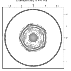
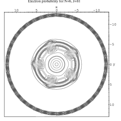
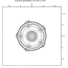
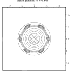
FIG. 5.: Comparsion of approximated charge distributions (in the rest frame of the minimal energy configuration) for $N=6$. Left are the distributions for filling factors $\nu=1/5$ (top) and $\nu=1/7$ (bottom) with $J=75$ and $J=105$ respectively. This is compared with the distributions for non-special magic numbers close to the special magic ones on the right. Note that no full restoration of symmetry occurs for $J=81$ (top), where the $j=1$ orbital can be seen to be occupied, but where the lowest-energy configuration barely sticks out of the more likely fully symmetric configuration. In case of $J=99$ (bottom), full symmetry restoration is still observed. See main text for details about which magic numbers fail to completely restore maximal symmetry.

approach. In particular, the radial distributions just become a bit more smeared out, but retain their qualitative structure.

Our results bring us to the conclusion that our hypothesis is a good one, i.e. that it predicts the correct qualitative behavior expected from quantum dots. It would hence be very interesting to derive this hypothesis from a microscopical treatment of quantum dots. It is well known that spin-spin and spin-orbit interactions are important in the theoretical understanding of electron orbitals of atoms. Quantum dots are often described as “artificial atoms” [6], and it would only further justify this labeling, if they indeed shared the importance of spin-interaction effects with their name-inducing natural relatives. Also, it would be interesting to relax our condition of completely polarized electrons in order to study quantum dots where angular momentum orbits can be occupied by upto two electrons. Finally, a more realistic normalization condition for the partition function, as mentioned above, might be desirable. But these investigations will be left for future work.

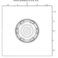
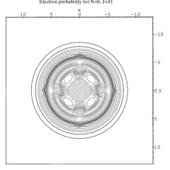
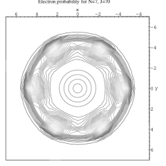
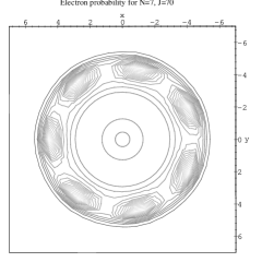
FIG. 6.: Comparsion of approximated charge distributions for different rest frames. Top row shows the quantum dot for $N=6$ and $J=81$ in the rest frames for full 6-fold symmetry (left) and for 4-fold symmetry (right), to be compared with the plot for 5-fold symmetry in figure 5 (top right). The fully symmetric configuration is still the dominant one. Bottom row shows a similar comparsion for $N=7$ and $J=70$ (the first magic number after the special magic number $J=63$ for $\nu=1/3$). The difference between the lowest energy rest frame (left) and the highest symmetry rest frame (right) is very small, but the latter is the dominant one. Hence, symmetry restoration still takes place, but is much weaker expressed than for other non-special magic numbers.

V Predictions

So far, we have successfully reproduced results which were already achieved by other methods, mainly by exact diagonalization techniques. Since our method is simple and fast, we can probe higher particle numbers and total angular momenta than the ones accessible to numerical methods. We will present here some calculations for $N=6$ with much larger total angular momentum as can be found in the literature (see figure 5).

In particular, we confirm that symmetry loss – as expected – occurs for higher special magic numbers corresponding to fillings $\nu=1/5$ and $\nu=1/7$. On the other hand, full ${{Z}}_{6}$ symmetry is still restored for most but not all non-special magic numbers! This is a new phenomenon, and also a nice demonstration of mesoscopic physics. Most non-special magic numbers do not contain states of the form $[(1,\bar{\jmath}_{1}),(N-1,\bar{\jmath}_{2})]$ with energies comparable to the (for magic numbers always existing) configuration $[(N,\bar{\jmath}=J/N)]$. The reason is that for most magic numbers there is no choice with very small $\bar{\jmath}_{1}$ which would favor a smaller energy than the energy of the $[(N,\bar{\jmath}=J/N)]$ configuration. One of the properties which make special magic numbers special is that at these values of the total angular momentum the configuration $[(1,0),(N-1,J/(N-1))]$ becomes possible.

However, if the total angular momentum $J$ is sufficiently large, configurations such as $[(1,1),(N-1,(J-1)/(N-1))]$ may have energies smaller than the energy of the most symmetric solution. In the case of $N=6$ this happens the first time for $J=81$, where the above given configuration consisting of a block with 5 particles around a single particle orbiting the center in the $j=1$ orbital has indeed a slightly lower energy than the configuration with a full block out of 6 particles, although the former state has a much smaller probability than the latter. This is simply due to the fact that for $J\gg 1$, the difference between the energies of the configurations $[(1,0),(N-1,J/(N-1))]$ and $[(1,1),(N-1,(J-1)/(N-1))]$ becomes arbitrarily small. Put differently, for $J\gg 1$ the system behaves more and more classical, but the transition from the quantum realm to the classical world is not continuous with increasing $J$. For example, full ${{Z}}_{6}$ symmetry is restored for the magic number $J=99$. More precisely, the first non-special magic numbers (1) where symmetry restoration does not take place are $J(N,k^{\prime}N)$ for $k^{\prime}\geq k^{\prime}_{0}(N)$. We have for example $k^{\prime}_{0}(6)=2$ and $k^{\prime}_{0}(7)=1$. These happen to be the non-special magic numbers which follow next to special magic numbers. For even higher $J$ we might expect that more and more magic numbers fail to restore the full symmetry of the system.

Because the minimal energy configuration does not possess the maximal possible symmetry, it may have a smaller probability than the maximal symmetric configuration due to different multiplicities. In fact, this is the case when the magic numbers are non-special. When the magic number is special, the minimal energy configuration is the dominant one, although the dominance is not strongly expressed – which is precisely the reason which leads to the droplet like probability distributions of such quantum dot states. It follows, that symmetry restoration should still work to some degree for the above discussed non-special magic numbers. We demonstrate this in figure 6, where we compare probability distributions for different rest frames, namely the rest frame of the minimal energy configuration and the one for the maximal symmetry configuration. One can infer from these plots that symmetry restoration does take place for the non-special magic numbers $J(N,k^{\prime}N)$, but of a somewhat lesser degree than for other non-special magic numbers.

Therefore, we have demonstrated that our method is capable of probing unknown regions in “quantum dot space” showing and predicting new patterns. We believe that our method is a useful tool to explore in more detail how quantum mechanics and classical physics are interlinked in mesoscopic systems.

REFERENCES

-
[1]
For a recent account, see for example
T. Chakraborty (ed.),
Proceedings of the workshop on
Novel Physics in Low Dimensional Electron Systems
(Dresden, July 27 – Aug 8, 1997),
to appear in Physica E.
Some other references are T.A. Fulton, G.J. Dolan, Phys. Rev. Lett 59 (1987) 59; U. Meirav et al., Z. Phys. B85 (1991) 357; H. Grabert, M.H. Devoret (eds.), Single Charge Tunneling, NATO ASI Series 294 (Plenum Press, 1992); M. Kastner, Physics Today (January 1993) 24; N.F. Johnson, J. Phys.: Condens. Matter 7 (1995) 965 - [2] Magic numbers were first found in numerical studies in S.M. Girvin, T. Jach, Phys. Rev. B28 (1983) 4506; P.A. Maksum, T. Chakraborty, Phys. Rev. Lett. 65 (1990) 108, Phys. Rev. B45 (1992) 1947.
- [3] So-called excited magic numbers with period were found in W.Y. Ruan et al., Phys. Rev. B51 (1995) 7942; P.A. Maksym, Phys. Rev. B53 (1996) 10871; T. Seki, Y Kuramoto, T. Nishino, J. Phys. Soc. Jpn. 65 (1996) 3945
- [4] Some references to analytical (for ) and numerical studies are U. Merkt, J. Huser, M. Wagner, Phys. Rev. B43 (1991) 7320; M. Taut, Phys. Rev. A (1993) 3561; P. Hawrylak, Phys. Rev. Lett. 71 (1993) 3347; A. Matulis, F.M. Peeters, J. Phys.: Condens. Matter 6 (1994) 7751 D. Pfannkuche, S.E. Ulloa, Phys. Rev. Lett. 74 (1995) 1194; A. Gonzalez, J. Phys.: Condens. Matter 9 (1997) 4643; E. Anisimova, A. Matulis, Energy Spectra of Few-Electron Quantum Dots, cond-mat/9711079; H. Imamura, P.A. Maksym, H. Aoki, Symmetry of ‘molecular’ configurations of interacting electrons in a quantum dot in strong magnetic fields, cond-mat/9712290; H. Imamura, H. Aoki, P.A. Maksym, Spin-Blockade in Single and Double Quantum Dots in Magnetic Fields: a Correlation Effect, cond-mat/9712291; A. Gonzalez, B. Partoens, A. Matulis, F.M. Peters, Ground-state energy of confined charged bosons in two dimensions, cond-mat/ 9806256; N. Akman, M. Tomak, Interacting electrons in a 2D quantum dot, cond-mat/9809192; C.E. Creffield, W. Häusler, J.H. Jefferson, S. Sarkar, Interacting electrons in polygonal quantum dots, cond-mat/9810096
- [5] G. Date, M.V.N. Murthy, R. Vathsan, Calssical Many-particle Clusters in Two Dimensions, cond-mat/9802034
-
[6]
M.A. Kastner,
Rev. Mod. Phys. 64 (1992) 849;
S. Tarucha, D.G. Austing, T. Honda,
Phys. Rev. Lett. 77 (1996) 3613;
Differences between atoms and quantum dots due to the nature of the confining potential are noted in J.H. Jefferson, W. Hausler, Quantum dots and artificial atoms, cond-mat/9705012