Nonlocal Effects on the Surface Resistance of High Temperature Superconductors with (100) and (110) Surfaces

Abstract

The low temperature surface resistance $R_{\text{s}}$ of $d$-wave superconductors is calculated as function of frequency assuming normal state quasiparticle mean free paths $\ell$ in excess of the penetration depth. Results depend strongly on the geometric configuration. In the clean limit, two contributions to $R_{\text{s}}$ with different temperature dependencies are identified: photon absorption by quasiparticles and pair breaking. The size of nonlocal corrections, which can be positive or negative depending on frequency decreases for given $\ell$ as the scattering phase shift $\delta_{\text{N}}$ is increased. However, except in the unitarity limit $\delta_{\text{N}}=0.5\,\pi$, nonlocal effects should be observable.

I INTRODUCTION

With the onset of superconductivity, a new length scale, the BCS coherence length $\xi_{{}_{0}}=v_{\text{F}}/\pi\Delta_{0}$ enters. [1] Its size, rather than the size of the normal state quasiparticle mean free path $\ell$, relative to the penetration depth $\lambda$ determines whether or not the electromagnetic response of the condensate is local. The situation is different for thermally exited quasiparticles which are responsible for losses at frequencies below the pair breaking threshold. These quasiparticles behave very much like quasiparticles in the normal state once the change in the density of states and the resulting change in thermal occupation of quasiparticle states are taken into account.[2] Hence one must expect to see nonlocal effects in the surface resistance of superconductors when $\ell\geq\lambda$. At finite frequencies the quasiparticles contribute to the screening currents so that there are some nonlocal corrections to the penetration depth of microwave fields as well.

High-$T_{\text{c}}$ materials are highly anisotropic. They can be viewed as stacks of weakly coupled conducting planes. In this paper we shall only consider the in-plane conductivity because it is only this component of the conductivity tensor which can be expected to show nonlocal effects. The in-plane coherence length typically is between 10 Å and 20 Å while the in-plane penetration depth is two orders of magnitude larger, so that high-$T_{\text{c}}$ superconductors are well into the London limit [1], $\xi_{{}_{0}}\ll\lambda$. While the quasiparticle in-plane mean free path $\ell$ is comparable to $\xi_{{}_{0}}$ near the transition temperature $T_{\text{c}}$, so that the corresponding scattering rate $\Gamma=v_{\text{F}}/2\ell$ is of the order of $T_{\text{c}}$, it is now generally accepted that $\ell$ increases substantially below $T_{\text{c}}$. [3, 4, 5, 6, 7] In high quality single crystals, the disorder induced mean free path $\ell^{\text{el}}$ can exceed the London penetration depth by quite a wide margin. [3, 4, 5, 27] In contrast to the normal state where a single parameter suffices to characterize the elastic scattering, both the concentration of scattering centers and the strength of the individual scatterer or, alternatively, the normal state elastic scattering rate $\Gamma$ and the scattering phase shifts have to be specified in the case of superconductors with unconventional[8] order parameters. We shall show below for the case of $s$-wave scattering that the scattering phase shift $\delta_{\text{N}}$ plays a very important role.

It has been pointed out by Chang and Scalapino [9] that nonlocal effects are absent when the conducting planes are parallel to the surface exposed to the microwave radiation ($\hat{c}$-axis orientation) because the spatial variation of the fields parallel to the surface occurs on length scales much larger than the penetration depth. Thus, for strictly 2 D quasiparticle motion, the scalar product ${\mathchoice{{\hbox{\boldmath$\displaystyle v$}}}{{\hbox{\boldmath$\textstyle v$}}}{{\hbox{\boldmath$\scriptstyle v$}}}{{\hbox{\boldmath$\scriptscriptstyle v$}}}}_{\text{F}}\cdot{\mathchoice{{\hbox{\boldmath$\displaystyle q$}}}{{\hbox{\boldmath$\textstyle q$}}}{{\hbox{\boldmath$\scriptstyle q$}}}{{\hbox{\boldmath$\scriptscriptstyle q$}}}}$ vanishes.

Zuccaro et al.[10] argued that, at least for YBa₂Cu₃O_7-δ (YBCO), coherent coupling between planes is not negligible so that there exists a finite component ${\mathchoice{{\hbox{\boldmath$\displaystyle v$}}}{{\hbox{\boldmath$\textstyle v$}}}{{\hbox{\boldmath$\scriptstyle v$}}}{{\hbox{\boldmath$\scriptscriptstyle v$}}}}_{\text{F}}^{\text{c}}$ of the Fermi velocity parallel to the surface normal. Assuming an isotropic gap, these authors calculated the nonlocal corrections to the surface impedance for parameters such that $\xi_{{}_{0}}\ll\lambda$. These calculations show the expected increase in the surface resistance in the anomalous skin effect regime $\omega\leq v_{\text{F}}/\lambda=(\xi_{{}_{0}}/\lambda)\pi\Delta_{0}\ll\Delta_{0}$ resulting from the direct absorption of photons by quasiparticles in an energy- and momentum-conserving process. Li et al.[11] also invoked finite dispersion perpendicular to the planes to argue that nonlocal effects prevent the observation of the nonlinear Meißner effect predicted by Yip and Sauls. [12] While this assumption of a 3 D tight-binding Fermi surface appears quite reasonable for YBCO, one nevertheless expects $\mathchoice{{\hbox{\boldmath$\displaystyle v$}}}{{\hbox{\boldmath$\textstyle v$}}}{{\hbox{\boldmath$\scriptstyle v$}}}{{\hbox{\boldmath$\scriptscriptstyle v$}}}_{\text{F}}^{\text{c}}\ll\mathchoice{{\hbox{\boldmath$\displaystyle v$}}}{{\hbox{\boldmath$\textstyle v$}}}{{\hbox{\boldmath$\scriptstyle v$}}}{{\hbox{\boldmath$\scriptscriptstyle v$}}}_{\text{F}}^{\text{ab}}$. Nonlocal effects will, therefore, be less significant for $\hat{c}$-axis oriented samples than for samples whose surfaces contain the $\hat{c}$-axis, like $\hat{a}$-axis oriented films or thin needles of single crystals with the $\hat{c}$-axis being the longest dimensions. Setting aside the problem of preparing high-quality $\hat{a}$-axis oriented films, microwave measurements of the surface impedance of such films are not well suited to a search for nonlocal effects because the typical current and field distributions [5] involve two vastly different components of the conductivity tensor. Transmission experiments in the THz regime, using linearly polarized light, would be more feasible.[13] For this reason we investigate the surface impedance for a rather broad range of frequencies. At very high frequencies, though, inelastic scattering would reduce the quasiparticle mean free paths even at low temperatures to such an extent that the local limit applies. An investigation of the electromagnetic response of a needle shaped single crystal to a parallel microwave magnetic field, which would involve the in-plane conductivity only, appears to be even more promising in view of the thick single crystals that can now be grown in BaZrO₃ crucibles. [14]

If the pairing state in high-$T_{\text{c}}$ superconductors has nodes, which is at present a widely held belief, then a momentum dependent coherence length could be introduced. This would exceed the penetration depth for momentum states in the nodal region so that high-$T_{\text{c}}$ materials are London superconductors only in the sense that for the majority of $\textstyle k$-states $\xi_{{}_{0}}(\mathchoice{{\hbox{\boldmath$\displaystyle k$}}}{{\hbox{\boldmath$\textstyle k$}}}{{\hbox{\boldmath$\scriptstyle k$}}}{{\hbox{\boldmath$\scriptscriptstyle k$}}})\ll\lambda$. This point was first raised by Kosztin and Leggett, [15] who found that the zero frequency clean limit penetration depth varies quadratically with temperature at very low temperatures, rather than linear which is considered to be a hallmark of $d$-wave superconductivity. This change in the temperature dependence of $\lambda$ due to nonlocality is however easily masked by mean free path and finite frequency effects.[5]

Schopohl and Dolgov[16] have argued that a linear temperature dependence of the penetration depth would violate the third law of thermodynamics. The nonlocal effects discovered by Kosztin and Leggett [15] could reconcile the $d$-wave model with this general thermodynamic argument but only for the geometry in which the $\hat{c}$-axis is parallel to the sample surface. Hirschfeld et al. [17] pointed out that the electromagnetic response kernel contains, in addition to the $\mathchoice{{\hbox{\boldmath$\displaystyle v$}}}{{\hbox{\boldmath$\textstyle v$}}}{{\hbox{\boldmath$\scriptstyle v$}}}{{\hbox{\boldmath$\scriptscriptstyle v$}}}_{\text{F}}\cdot\mathchoice{{\hbox{\boldmath$\displaystyle q$}}}{{\hbox{\boldmath$\textstyle q$}}}{{\hbox{\boldmath$\scriptstyle q$}}}{{\hbox{\boldmath$\scriptscriptstyle q$}}}$ term, a term $q^{2}/2m$ which leads to nonlocal corrections at some very low temperatures in any geometry. For $q\approx 1/\lambda\ll k_{\text{F}}$ this term can usually be neglected and this is what we shall do here because we are interested in microwave losses at low but finite temperatures. For strictly 2 D systems, one might wonder whether fluctuation effects would not be much more important than such very small nonlocal corrections.

Another consequence of $d$-wave pairing is the fact that pair-breaking is possible at any frequency. However, for this process to contribute to the transverse conductivity, the finite photon momentum needs to be taken into account unless the required momentum transfer is provided by some other scattering event occuring simultaneously. Since we are interested here in low temperatures, we shall only consider disorder induced elastic scattering. If only $s$-wave scattering is taken into account, it is easy enough to write down a general expression for the complex conductivity $\sigma(\mathchoice{{\hbox{\boldmath$\displaystyle q$}}}{{\hbox{\boldmath$\textstyle q$}}}{{\hbox{\boldmath$\scriptstyle q$}}}{{\hbox{\boldmath$\scriptscriptstyle q$}}},\omega)$. In order to isolate the two contributions to the surface resistance which are due to nonlocality, we shall also consider the clean limit.

II THEORY, GENERAL CASE

The current-current correlation function from which the transverse conductivity is derived according to

$$\sigma({\mathchoice{{\hbox{\boldmath$\displaystyle q$}}}{{\hbox{\boldmath$\textstyle q$}}}{{\hbox{\boldmath$\scriptstyle q$}}}{{\hbox{\boldmath$\scriptscriptstyle q$}}}},\omega)=-\frac{e^{2}}{i\omega}\,\left\{\frac{n}{m}+\big{\langle}[j_{y},j_{y}]\big{\rangle}(\mathchoice{{\hbox{\boldmath$\displaystyle q$}}}{{\hbox{\boldmath$\textstyle q$}}}{{\hbox{\boldmath$\scriptstyle q$}}}{{\hbox{\boldmath$\scriptscriptstyle q$}}},\omega)\right\}\,,$$ (1)

can be expressed very simply in terms of normal and anomalous single particle Green’s functions [18]

$$\big{\langle}[j_{y},j_{y}]\big{\rangle}(\mathchoice{{\hbox{\boldmath$\displaystyle q$}}}{{\hbox{\boldmath$\textstyle q$}}}{{\hbox{\boldmath$\scriptstyle q$}}}{{\hbox{\boldmath$\scriptscriptstyle q$}}},i\nu_{m})=2T\sum_{\omega_{n}}\int\frac{d^{D}p}{(2\pi)^{D}}\,\frac{p_{y}^{2}}{m^{2}}\,\times$$ (3)

$$\times\Big{[}{\cal G}_{\omega_{n}}(\mathchoice{{\hbox{\boldmath$\displaystyle p$}}}{{\hbox{\boldmath$\textstyle p$}}}{{\hbox{\boldmath$\scriptstyle p$}}}{{\hbox{\boldmath$\scriptscriptstyle p$}}})\,{\cal G}_{\omega_{n}-\nu_{m}}(\mathchoice{{\hbox{\boldmath$\displaystyle p$}}}{{\hbox{\boldmath$\textstyle p$}}}{{\hbox{\boldmath$\scriptstyle p$}}}{{\hbox{\boldmath$\scriptscriptstyle p$}}}\!-\!\mathchoice{{\hbox{\boldmath$\displaystyle q$}}}{{\hbox{\boldmath$\textstyle q$}}}{{\hbox{\boldmath$\scriptstyle q$}}}{{\hbox{\boldmath$\scriptscriptstyle q$}}})+{\cal F}_{\omega_{n}}(\mathchoice{{\hbox{\boldmath$\displaystyle p$}}}{{\hbox{\boldmath$\textstyle p$}}}{{\hbox{\boldmath$\scriptstyle p$}}}{{\hbox{\boldmath$\scriptscriptstyle p$}}})\,{\cal F}_{\omega_{n}-\nu_{m}}(\mathchoice{{\hbox{\boldmath$\displaystyle p$}}}{{\hbox{\boldmath$\textstyle p$}}}{{\hbox{\boldmath$\scriptstyle p$}}}{{\hbox{\boldmath$\scriptscriptstyle p$}}}\!-\!\mathchoice{{\hbox{\boldmath$\displaystyle q$}}}{{\hbox{\boldmath$\textstyle q$}}}{{\hbox{\boldmath$\scriptstyle q$}}}{{\hbox{\boldmath$\scriptscriptstyle q$}}})\Big{]}\,,$$

when there are no vertex corrections. This is the case for isotropic disorder induced scattering, which we will focus on here. Momentum dependent inelastic interactions, capable of causing the formation of unconventional superconducting pair states, do require consideration of vertex corrections. [19] At low temperatures and low frequencies, however, the contributions of these interactions to the quasiparticle lifetimes are negligible. All the complications resulting from quasiparticles in an unconventional superconductor being scattered off point defects, which were first discussed in the context of Heavy Fermion superconductors, [8] affect only the single particle selfenergies discussed below.

The momentum integral in Eq. (3) is evaluated under the assumption that the main contribution comes from quasiparticle states near the Fermi surface. We consider purely two-dimensional conduction and simplify the 2D Fermi surface to a circle. The Fermi velocity $v_{\text{F}}$ and the density of states per spin at the Fermi level $N(0)=m/2\pi$ are combined into a single parameter, the plasma wavelength $\lambda_{\text{p}}$, according to

$$\frac{1}{\mu_{{}_{0}}\lambda_{\text{p}}^{2}}=e^{2}\,N(0)\,v_{\text{F}}^{2}\frac{1}{s}\,,$$ (4)

where $s$ is the average distance between conducting planes. In the clean limit, $\lambda_{\text{p}}$ is identical to the zero temperature London penetration depth $\lambda_{\text{L}}$. With these assumptions one obtains for the conductivity after analytic continuation of $i\nu_{m}$ to the real axis

$$\sigma(\mathchoice{{\hbox{\boldmath$\displaystyle q$}}}{{\hbox{\boldmath$\textstyle q$}}}{{\hbox{\boldmath$\scriptstyle q$}}}{{\hbox{\boldmath$\scriptscriptstyle q$}}},\omega)=\frac{1}{\mu_{{}_{0}}\lambda_{\text{p}}^{2}}\,\frac{1}{2\omega}\,\int_{-\omega/2}^{+\infty}d\Omega\int_{0}^{2\pi}\frac{d\varphi}{2\pi}\,\sin^{2}\varphi$$ (10)

$$\bigg{\{}\;\;\,\tanh\frac{\Omega+\omega}{2T}\,2i\,{\rm Im}\,M(\varphi;\mathchoice{{\hbox{\boldmath$\displaystyle q$}}}{{\hbox{\boldmath$\textstyle q$}}}{{\hbox{\boldmath$\scriptstyle q$}}}{{\hbox{\boldmath$\scriptscriptstyle q$}}};\Omega_{+}+\omega,\Omega_{+})$$

$$\;-\left[\tanh\frac{\Omega\!+\!\omega}{2T}-\tanh\frac{\Omega}{2T}\right]\,M(\varphi;\mathchoice{{\hbox{\boldmath$\displaystyle q$}}}{{\hbox{\boldmath$\textstyle q$}}}{{\hbox{\boldmath$\scriptstyle q$}}}{{\hbox{\boldmath$\scriptscriptstyle q$}}};\Omega_{+}+\omega,\Omega_{+})$$

$$\;+\left[\tanh\frac{\Omega\!+\!\omega}{2T}-\tanh\frac{\Omega}{2T}\right]\,M(\varphi;\mathchoice{{\hbox{\boldmath$\displaystyle q$}}}{{\hbox{\boldmath$\textstyle q$}}}{{\hbox{\boldmath$\scriptstyle q$}}}{{\hbox{\boldmath$\scriptscriptstyle q$}}};\Omega_{+}+\omega,\Omega_{-})\bigg{\}}$$

where $+(-)$ indicates a positive (negative) infinitesimal imaginary part. $M$ is an abbreviation for

$$M(\varphi;\mathchoice{{\hbox{\boldmath$\displaystyle q$}}}{{\hbox{\boldmath$\textstyle q$}}}{{\hbox{\boldmath$\scriptstyle q$}}}{{\hbox{\boldmath$\scriptscriptstyle q$}}};\Omega_{+}+\omega,\Omega_{\pm})=$$ (15)

$$\left.\left(1+\frac{(\Omega+\omega)\,Z(\Omega_{+}+\omega)\,\Omega\,Z(\Omega_{\pm})+\Delta^{2}(\varphi)}{R_{1}\,R_{2}}\right.\right)\times$$

$$\times\frac{R_{1}+R_{2}}{\big{[}R_{1}+R_{2}\big{]}^{2}+\big{[}\,v_{\text{F}}q\cos\varphi+\chi(\Omega_{\pm})-\chi(\Omega_{+}+\omega)\big{]}^{2}}$$

where

$$\begin{array}[]{rcl}R_{1}&=&\displaystyle\sqrt{\Delta^{2}(\varphi)-\big{(}\Omega\,Z(\Omega_{\pm})\big{)}^{2}}\,,\\ R_{2}&=&\displaystyle\sqrt{\Delta^{2}(\varphi)-\big{(}(\Omega+\omega)\,Z(\Omega_{+}+\omega)\big{)}^{2}}\,.\end{array}$$ (16)

The order parameter, which is assumed to have d${}_{x^{2}-y^{2}}$-symmetry with the respect to the crystallographic axes, is represented as

$$\Delta(\varphi)=\Delta_{0}(T)\,\cos 2(\varphi\!-\!\varphi_{{}_{0}})\,,$$ (17)

where $\varphi_{{}_{0}}$ is the angle between the crystallographic (100)-axis and the surface normal. In the local limit, the orientation of the order parameter relative to the sample surface has no effect on the conductivity, provided one neglects the suppression of the order parameter by the surface[21] which occurs on a length scale $\xi_{{}_{0}}\ll\lambda_{\text{p}}$. The $\varphi$-integral can then be reduced to the interval $[0,\pi/2]$. In the nonlocal case with $\varphi_{{}_{0}}$ arbitrary such a reduction produces four different terms. For the exceptional cases $\varphi_{{}_{0}}=0$ [(100)-oriented surface] and $\varphi_{{}_{0}}=\pi/4$ [(110)-oriented surface], these terms are pairwise equal. Further simplification is possible in the clean limit (see next section), as well as in the strong and weak scattering limit, because in these limits the selfenergy $\chi$ either vanishes or becomes independent of $\Omega$, so that $M$ depends only on $\left[\,v_{\text{F}}q\cos\varphi\right]^{2}$.

The dependence of $M$ on $\textstyle q$ is very simple because we neglected $\textstyle q$ in the argument of the order parameter and the other self-energies. Anticipating $|\mathchoice{{\hbox{\boldmath$\displaystyle q$}}}{{\hbox{\boldmath$\textstyle q$}}}{{\hbox{\boldmath$\scriptstyle q$}}}{{\hbox{\boldmath$\scriptscriptstyle q$}}}|\approx 1/\lambda_{\text{p}}$ this is justified. If one wanted to keep, in addition to $v_{\text{F}}q\cos\varphi$, the term $q^{2}/2m$,[17] such an approximation would be inconsistent. For $q\approx k_{\text{F}}$ the response of a $d$-wave superconductor changes its character completely, because the coherence factors would revert from case II to case I.[1, 22]

Because of the restriction to $s$-wave scattering there are no self-energy corrections to the $d$-wave order parameter. The remaining selfenergy corrections are to be determined from

$$\Omega Z(\Omega_{\pm})=\Omega+\Gamma_{\text{N}}^{\text{el}}\frac{\langle g_{{}_{0}}(\varphi,\Omega_{\pm}\!)\rangle}{\cos^{2}\delta_{\text{N}}\!-\!\sin^{2}\delta_{\text{N}}\langle g_{{}_{0}}(\varphi,\Omega_{\pm}\!)\rangle^{2}}$$ (18)

and

$$\chi(\Omega_{\pm})=\Gamma_{\text{N}}^{\text{el}}\,\frac{\cot\delta_{\text{N}}}{\cos^{2}\delta_{\text{N}}-\sin^{2}\delta_{\text{N}}\langle g_{{}_{0}}(\varphi,\Omega_{\pm}\!)\rangle^{2}}$$ (19)

$\langle g_{{}_{0}}\rangle$ is the energy-integrated normal Green’s functions, averaged over the Fermi circle

$$\langle g_{{}_{0}}(\varphi,\Omega_{\pm})\rangle=\int\limits_{0}^{2\pi}\frac{d\varphi}{2\pi}\frac{\Omega Z(\Omega_{\pm})}{\sqrt{\Delta^{2}(\varphi)-\left(\Omega Z(\Omega_{\pm})\right)^{2}}}$$ (20)

$$\Gamma_{\text{N}}^{\text{el}}=n_{\text{imp}}\,\frac{\pi N(0)v^{2}}{1+\left(\pi N(0)v\right)^{2}}=\frac{n_{\text{imp}}}{\pi N(0)}\,\sin^{2}\delta_{\text{N}}$$ (21)

is the elastic scattering rate in the normal state and $\delta_{\text{N}}=\tan^{-1}(\pi N(0)v)$ is the scattering phase shift.

From $\sigma(\mathchoice{{\hbox{\boldmath$\displaystyle q$}}}{{\hbox{\boldmath$\textstyle q$}}}{{\hbox{\boldmath$\scriptstyle q$}}}{{\hbox{\boldmath$\scriptscriptstyle q$}}}=q\hat{e}_{z}\,,\,\omega)$ the surface impedance is calculated assuming specular reflection

$${\cal Z}_{\text{s}} = R_{\text{s}}(\omega)-i\omega\mu_{{}_{0}}\lambda(\omega)$$ (22)

$$= -i\omega\mu_{{}_{0}}\,\frac{2}{\pi}\,\int\limits_{0}^{\infty}\frac{dq}{q^{2}-i\omega\mu_{{}_{0}}\sigma(q,\omega)}\;.$$ (23)

We have not evaluated the formula applicable for diffuse surface scattering for lack of computer time.

III THEORY, CLEAN LIMIT

Since we are primarily interested in the surface resistance, we shall calculate only the real part $\sigma_{1}$ of the complex conductivity Eq. (1). The imaginary part $\sigma_{2}$ should simply be given by[1, 5] $1/\omega\mu_{{}_{0}}\lambda_{\text{p}}^{2}$ and this expectation is borne out by the numerical calculations based on the general formalism presented in the previous section. Inserting spectral representations for the Green’s functions, evaluating the sum over Matsubara frequencies $\omega_{n}$ and performing the analytic continuation with respect to $i\nu_{m}$ we obtain

$$\sigma_{1}(\mathchoice{{\hbox{\boldmath$\displaystyle q$}}}{{\hbox{\boldmath$\textstyle q$}}}{{\hbox{\boldmath$\scriptstyle q$}}}{{\hbox{\boldmath$\scriptscriptstyle q$}}},\omega)=\frac{1}{\mu_{{}_{0}}\lambda_{\text{p}}^{2}}\,\frac{1}{\omega}\,\int\limits_{-\omega/2}^{\infty}d\Omega\big{[}f(\Omega)-f(\Omega+\omega)\big{]}\times$$ (24)

$$\times \int\limits_{0}^{2\pi}d\varphi\,\sin^{2}\varphi\,I_{j}\Big{[}\Omega,\Omega+\omega,v_{\text{F}}q\cos\varphi,\Delta(\varphi)\Big{]}$$ (25)

with

$$I_{j} = \frac{\pi}{4}\int\limits_{-\infty}^{\infty}\frac{d\xi}{2\pi}\Big{[}\mbox{Im}\,G_{\Omega_{+}}(\xi)\,\mbox{Im}\,G_{\Omega_{+}-\omega}(\xi-v_{\text{F}}q\cos\varphi)$$ (27)

$${}+\mbox{Im}\,F_{\Omega_{+}}(\xi)\,\mbox{Im}\,F_{\Omega_{+}-\omega}(\xi-v_{\text{F}}q\cos\varphi)\Big{]}\,.$$

Since

$$\mbox{Im}\,G_{\Omega_{+}}(\xi)=-\frac{\pi}{2}\times$$ (29)

$$\sum_{\sigma=\pm 1}\left(\sigma+\frac{\Omega}{\sqrt{\Omega^{2}-\Delta^{2}}}\right)\delta\left(\xi-\sigma\sqrt{\Omega^{2}-\Delta^{2}}\right)$$

the energy integral is easily done, yielding

$$I_{j}=\frac{\Omega}{|\Omega|}\times$$ (31)

$$\;\sum_{\sigma=\pm 1}\left(\sigma+\frac{\Omega(\Omega+\omega)+\Delta^{2}}{\sqrt{\Omega^{2}-\Delta^{2}}\sqrt{(\Omega+\omega)^{2}-\Delta^{2}}}\right)\delta\big{[}g_{\sigma}(\Omega)\big{]}$$

where

$$g_{\sigma}(\Omega) = v_{\text{F}}q\cos\varphi-\sqrt{(\Omega+\omega)^{2}-\Delta^{2}(\varphi)}$$ (33)

$${}+\sigma\sqrt{\Omega^{2}-\Delta^{2}(\varphi)}$$

So far, the evaluation of $\sigma_{1}$ is equivalent to that given by Mattis and Bardeen[23] who, at this point, take the extreme anomalous limit, i.e. they neglect the $\Omega$-dependence of $g_{\sigma}$. If this approximation were used in the case of a $d$-wave superconductor with nodal lines parallel to the surface, the normal state conductivity $\sigma_{1}=\frac{3\pi}{4}\,\frac{1}{\mu_{{}_{0}}\lambda_{\text{p}}^{2}}\,\frac{1}{v_{\text{F}}q}$, appropriate for the anomalous skin effect regime, would be obtained. Since HTC materials are essentially London superconductors, taking this limit is not justifiable. Instead, we shall find the zeros of $g_{\sigma}(\Omega)$ and perform the $\Omega$-integral. In this way we cannot reproduce the normal state result because, for $\Delta\to 0$, $g_{\sigma}$ becomes either independent of $\Omega$ or the $\delta$-functions give a vanishing contribution.

However, the same approach is used successfully in the theory of the electronic Raman response of high temperature superconductors, which involves a density-density correlation function with some vertex $\gamma(\varphi)$ specific to the Raman response in place of the current vertex $p_{y}/m$. The important difference is that the coherence factor is case I,[1] i.e. $\Delta^{2}$ in the numerator of Eqs. (15,31) has a different sign. One can then take the local limit $q\to 0$ and evaluate the frequency integral using $g_{-1}(-\omega/2)=0$ with the result

$$-\,{\rm Im}\,\big{\langle}[n,n]\big{\rangle}\left(0,\omega\right)=\frac{2N(0)}{\omega}\,\tanh\left(\frac{\omega}{4T}\right)\times$$ (35)

$$\quad\times\int\limits_{0}^{\pi/2}d\varphi\,\gamma^{2}\left(\varphi\right)\big{[}2\Delta\left(\varphi,T\right)\big{]}^{2}\frac{\theta\,\big{[}\,\omega\!-\!|2\Delta\!\left(\varphi,T\right)\!|\big{]}}{\sqrt{\omega^{2}\!-\!\left[2\Delta\!\left(\varphi,T\right)\right]^{2}}}\,.$$

This pair breaking contribution to the Raman response does account quite successfully [24, 25] for a range of experimental observations. The corresponding result for $\sigma_{1}$ is, of course, zero. This difference in the local clean limit explains why the absorption of low frequency photons by charge carriers in high temperature superconductors depends much more strongly on quasiparticle mean free paths than the inelastic scattering of such photons. [26]

Solving $g_{\pm 1}(\Omega)=0$ in the interval $[-\omega/2,\infty]$ leads to

$$\Omega_{0}(\varphi)=-\frac{\omega}{2}+\frac{1}{2}v_{\text{F}}q\cos\varphi\sqrt{1-\frac{[2\Delta(\varphi)]^{2}}{\omega^{2}-[v_{\text{F}}q\cos\varphi]^{2}}}\;.$$ (36)

For $g_{+1[-1]}\big{(}\Omega_{0}(\varphi)\big{)}$ to vanish, $\omega\sqrt{1-\frac{[2\Delta(\varphi)]^{2}}{\omega^{2}-[v_{\text{F}}q\cos\varphi]^{2}}}$ must be greater [less] than $v_{\text{F}}q\cos\varphi$ so that either $\delta\left[g_{+1}\right]$ or $\delta\left[g_{-1}\right]$ contributes. $\Omega_{0}(\varphi)$ must be real, which requires

$$1-\frac{[2\Delta(\varphi)]^{2}}{\omega^{2}-[v_{\text{F}}q\cos\varphi]^{2}}\geq 0\;.$$ (37)

For $\cos\varphi>\frac{\omega}{v_{\text{F}}q}$ this is always fulfilled, irrespective of the magnitude and $\varphi$-dependence of the order parameter. $\Omega_{0}(\varphi)$ is positive for such $\varphi$ so that this represents the quasiparticle contribution to $\sigma_{1}$ which, because of the Fermi function in (24), becomes small at low temperatures. In the opposite case $\Omega_{0}(\varphi)$ is negative. The inequality (37) then leads to the usual condition $\omega>2\Delta$ for pair breaking, when the order parameter is isotropic. For a $d$-wave superconductor, $\Delta(\varphi)$ has to be specified at this point. We introduce the abbreviations

$$t\equiv\cos\varphi,\quad y\equiv\left[\frac{2\Delta_{0}(T)}{\omega}\right]^{2},\quad x\equiv\left[\frac{v_{\text{F}}q}{\omega}\right]^{2}\;.$$ (38)

For a (100)-surface we can then write

$$\Delta(\varphi)=\Delta_{0}(T)\left[2t^{2}-1\right]\;.$$ (39)

For this orientation of the $d$-wave order parameter the inequality (37) is fulfilled for $t\in\left[t_{\text{min}},t_{\text{max}}\right]$ with

$$t_{\text{min}}=$$ (41)

$$\max\left\{0,\left[\textstyle\frac{1}{2}\left(1-\frac{x}{4y}\right)-\frac{1}{2}\sqrt{\left(1-\frac{x}{4y}\right)^{2}\!+\frac{1}{y}-1}\right]^{\frac{1}{2}}\right\}\!$$

$$t_{\text{max}}=$$ (43)

$$\min\left\{1,\left[\textstyle\frac{1}{2}\left(1-\frac{x}{4y}\right)+\frac{1}{2}\sqrt{\left(1-\frac{x}{4y}\right)^{2}\!+\frac{1}{y}-1}\right]^{\frac{1}{2}}\right\}\!.$$

Such an interval exists only if the square root is real. For $y\leq 1\Longleftrightarrow\omega\geq 2\Delta_{0}$ this is always the case. For $y>1$, the interval is empty if $x>4y$. For $x<4y$, the square root is real provided $x\leq 4y\left[1-\sqrt{1-1/y}\right]$. For $\omega\ll 2\Delta_{0}$ this limits the $q$-integration in Eq. (23) to the interval $\left[0,\sqrt{2}\omega\right]$.

Combining Eqs. (24), (31), and (36) we obtain

$$\sigma_{1}(\mathchoice{{\hbox{\boldmath$\displaystyle q$}}}{{\hbox{\boldmath$\textstyle q$}}}{{\hbox{\boldmath$\scriptstyle q$}}}{{\hbox{\boldmath$\scriptscriptstyle q$}}},\omega)=\frac{2(2\Delta_{0}(T))^{2}}{\mu_{{}_{0}}\lambda_{\text{p}}^{2}\omega}\times$$ (47)

$$\times\left[\Theta\Big{(}\sqrt{2}\omega-v_{\text{F}}q\Big{)}\int\limits_{t_{\text{min}}}^{t_{\text{max}}}dt+\Theta\Big{(}v_{\text{F}}q-\omega\Big{)}\int\limits_{\frac{\omega}{v_{\text{F}}q}}^{1}dt\right]\times$$

$$\times\sqrt{1-t^{2}}\Big{[}f\big{(}\Omega_{0}(t)\big{)}-f\big{(}\omega+\Omega_{0}(t)\big{)}\Big{]}\times$$

$$\times\frac{(v_{\text{F}}qt)^{3}\left[2t^{2}-1\right]^{2}}{\big{[}\omega^{2}-(v_{\text{F}}qt)^{2}\big{]}^{2}\big{[}2\Omega_{0}(t)+\omega\big{]}}$$

where the first integral represents the pair breaking contribution while the second represents the contribution from quasiparticles.

For a (110)-surface, $\Delta(\varphi)=\Delta_{0}(T)\,\sin 2\varphi$, so that the factor $\left[2t^{2}-1\right]^{2}$ in (47) has to be replaced by $4\left(1-t^{2}\right)t^{2}$. The limits of integration in the pair breaking contributions also need to be changed. Instead of the interval $\left[t_{\text{min}},t_{\text{max}}\right]$ around $\varphi=\pi/4$ we now have two intervals $t\in\left[0,t_{\text{min}}^{\prime}\right]$ and $t\in\left[t_{\text{max}}^{\prime},1\right]$ near $\varphi=0$ and $\varphi=\pi/2$ which can contribute to $\sigma_{1}$. $t_{\text{min}}^{\prime}$and $t_{\text{max}}^{\prime}$ are given by expressions very similar to (41) and (43).

IV Results and Discussion

Parameters required as input for the numerical calculations are the plasma wavelength $\lambda_{\text{p}}$, the in-plane Fermi velocity $v_{\text{F}}$, the transition temperature $T_{\text{c}}$ and the order parameter amplitude $\Delta_{0}(T=0)$. The values chosen are typical of YBCO:[5] $T_{\text{c}}=90.5$ K, $v_{\text{F}}=1.4\cdot 10^{7}$ cm/s, $\lambda_{\text{p}}=140$ nm, and $2\Delta_{0}(T=0)/T_{\text{c}}=7.4$. Because of (4), $v_{\text{F}}$ and $\lambda_{\text{p}}$ are not entirely independent. The values given are consistent with an effective mass $m\approx 3\,m_{0}$. $T_{\text{c}}$ sets the temperature scale but is irrelevant otherwise. The rather large value of $\Delta_{0}(T=0)$ is deduced from the sharp drop in $R_{\text{s}}$ and $\lambda(T)$ observed in the vicinity of $T_{\text{c}}$. If this were attributable to a non-BCS temperature dependence of $\Delta_{0}(T)$, a smaller value of $\Delta_{0}(T=0)$ could be inferred which would increase all theoretical predictions for the low temperature surface resistance.

$\lambda_{\text{p}}$ and $v_{\text{F}}$ are the parameters which control the importance of nonlocal effects. We have performed some calculations with $\lambda_{\text{p}}=100$nm. Since in the local limit $R_{\text{s}}=0.5\,\omega^{2}\mu_{{}_{0}}^{2}\lambda_{\text{p}}^{3}\sigma_{1}$ is proportional to $\lambda_{\text{p}}$ one has to scale $R_{\text{s}}^{\text{local}}$ with $\lambda_{\text{p}}$ to appreciate the differences in the nonlocal results. Because the effect of modest changes in $\lambda_{\text{p}}$ are rather obvious, we shall not display these results.

Fig. 1 shows results for $R_{\text{s}}$ at temperatures $T=0.13\,T_{\text{c}}$ and $T=0.05\,T_{\text{c}}$ for a disorder induced scattering rate $\Gamma=0.1\,$meV, which would correspond to a normal state mean free path of 460 nm. The scattering phase shift has been chosen as $\delta_{\text{N}}=0$ (Born approximation). Allowing for nonlocality yields peaks in $R_{\text{s}}$ at around 100 GHz which greatly exceed the results in the local limit. The peak heights decrease rapidly with decreasing temperature, which indicates that these contributions to $R_{\text{s}}$ are due to direct photon absorption by thermally excited quasiparticles. This process ceases to be effective when $\omega\gg v_{\text{F}}q$. With $q\approx 1/\lambda_{\text{p}}$ we estimate that this “anomalous skin effect regime” should end at frequencies around $\nu\geq v_{\text{F}}/2\pi\lambda_{\text{p}}\approx 160\,$GHz in agreement with our numerical calculations. It is remarkable that here we have a range of frequencies in which $R_{\text{s}}$ is predicted to drop quite rapidly.

FIG. 1.: Surface resistance as function of frequency for two temperatures, $T/T_{\text{c}}=0.13$ (dashed lines) and $T/T_{\text{c}}=0.05$ (dot-dashed and dot-dot-dashed lines), for a $d_{x^{2}-y^{2}}$ order parameter with its lobes perpendicular and parallel to the surface. The dotted line is the contribution to $R_{\text{s}}$ from pair breaking in the clean limit. The solid line represents the sum of this dotted line and the dot-dot-dashed line.

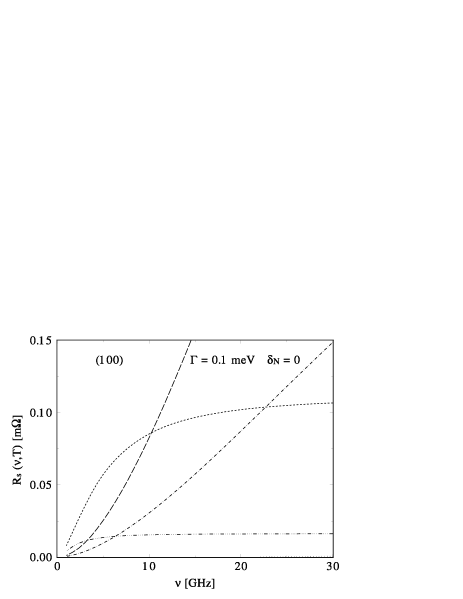
FIG. 2.: Blow-up of the low frequency section of Fig. 1. Pair breaking effects are negligible at these frequencies.

At higher frequencies, $R_{\text{s}}$ increases again but is essentially temperature independent. This, one would suspect, is the contribution to $R_{\text{s}}$ from pair breaking. To check this, we calculated the pair breaking contribution in the clean limit from (47). The result is shown as dotted line. Taking the sum of this contribution and the result of the local approximation at $T=0.04\,T_{\text{c}}$ gives the solid line, which reproduces the result of the full nonlocal calculation remarkably well. The increase in $R_{\text{s}}$ found in the local approximation must also be attributed to pair breaking, made possible by the $d$-wave character of the pair state and the momentum uncertainty due to static disorder.

While Fig. 1 shows the expected increase in $R_{\text{s}}$, a completely different picture emerges when the same results are replotted for the small range of microwave frequencies relevant for applications (Fig. 2). Here we see that, depending on temperature, there exists a frequency below which $R_{\text{s}}$ in the local limit exceeds the results from the nonlocal calculation. This is a consequence of the particular orientation of the order parameter we assumed. At these low frequencies the term $v_{\text{F}}q\cos\varphi$ in (15) emphasizes the contribution from quasiparticles moving parallel to the surface. Since this is the direction in which the order parameter has its maximum, the number of occupied $\textstyle k$-states, that are effective in the absorption process, is reduced. The change in sign of the nonlocal correction to $R_{\text{s}}$ with frequency would help to explain why theoretical predictions based on the local limit are higher than the low temperature data taken by Bonn et al.[4] on untwinned YBCO single crystals at 4.13 GHz and lower than those taken at 34.8 GHz.[27]

When $R_{\text{s}}$ becomes independent of frequency in the local limit, $\sigma_{1}$ must vary as $1/\omega^{2}$. In the normal state this would be the case for frequencies such that $\omega/2\Gamma\gg 1$, for parameters used here $\nu\gg 50\,$GHz. In the superconducting state, the effective scattering rate, which for given microwave frequency involves some temperature dependent frequency average,[28, 5] depends very sensitively on $\delta_{\text{N}}$. For $\delta_{\text{N}}=\pi/2$ it is usually found to be larger than $\Gamma$, while for $\delta_{\text{N}}=0$ it is much less than $\Gamma$ [Ref. [5], Figs. 14 and 19]. Since $\delta_{\text{N}}=0$ was chosen to obtain the data shown in Figs. 1 and 2, it is not surprising that $R_{\text{s}}$ becomes frequency independent at frequencies much lower than the 50 GHz estimated above. Since the surface resistance in $\hat{c}$-axis oriented samples, where we believe the local limit to apply, does increase between 1 GHz and 87 GHz, we must conclude that the scattering phase shift is closer to $\pi/2$ than 0.

The fact that the full nonlocal results for $R_{\text{s}}$ are lower at low frequencies than results obtained by taking the local limit does not depend in any essential way on the scattering rate or the scattering phase shift. This can be seen from Fig. 3 where both types of results, obtained for a range of scattering rates $\Gamma$ and $\delta_{\text{N}}=0.4\,\pi$, are compared in a double logarithmic plot. While $R_{\text{s}}$ depends very sensitively on $\Gamma$ in the local limit, it is very nearly independent of scattering when nonlocality is taken into account, as one would expect in the extreme anomalous limit. Perhaps surprisingly then, and contrary to the behavior in the normal state, it is $R_{\text{s}}^{\text{local}}$ that moves towards $R_{\text{s}}^{\text{nonlocal}}$ to close the gap between the two, when $\Gamma$ increases. Unlike the high frequency regime shown in Fig. 1, $R_{\text{s}}$ at these microwave frequencies is certainly not the sum of two independent contributions. The dotted line is the local result for the lower temperature already shown in Fig. 1. Comparison with the other local curves indicates that in the superconducting state a small scattering phase shift is indeed more or less equivalent to a much reduced normal state scattering rate together with a large scattering phase shift.

FIG. 3.: Double logarithmic plot of the local and nonlocal surface resistance for frequencies 1 GHz $\leq\nu\leq 100\,$GHz and for different scattering rates $\Gamma$. The curves marked with numbers are the results of the local approximations. The numbers themselves are the values of $\Gamma$ in [meV] used in the calculations. The four corresponding results of the fully nonlocal theory are those which attain the lowest values at 1 GHz. The dotted curve is the local result for $\Gamma=0.1\,$meV and $\delta_{\text{N}}=0$.

FIG. 4.: Surface resistance as function of the scattering rate for two different scattering phase shifts for fixed frequency $\nu=20\,$GHz. The inset shows $R_{\text{s}}$ for $\delta_{\text{N}}=0.4\,\pi$ at $\nu=220\,$GHz. Local results are those that vanish for $\Gamma\to 0$. The temperature is $T/T_{\text{c}}=0.04$.

The dependence of $R_{\text{s}}$ on $\Gamma$ and $\delta_{\text{N}}$ at a fixed frequency is further elucidated in the main frame of Fig. 4. In the unitarity limit $\delta_{\text{N}}=0.5\,\pi$, nonlocal effects vanish for $\Gamma\geq 0.1\,$meV. In this case the value of $R_{\text{s}}$ can be calculated from the “universal” conductivity $\sigma_{00}=1/\mu_{{}_{0}}\lambda_{\text{p}}^{2}\pi\Delta_{0}(0)$.[29] In the local limit, $R_{\text{s}}$ must vanish for $\Gamma\to 0$. Before it does so, $R_{\text{s}}(\Gamma)$ goes through a maximum, whose height, width and position depend sensitively on $\delta_{\text{N}}$. Because of this behavior one can fit the low temperature surface resistance of high quality YBCO samples by choosing a small value of $\Gamma$ which is, however, still compatible with the expected structural disorder, and then adjusting the scattering phase shift.[5] With nonlocality taken into account, $R_{\text{s}}$ has a finite limit for $\Gamma\to 0$, as in the normal state. At the lower end of the microwave regime $R_{\text{s}}^{\text{nonlocal}}\gg R_{\text{s}}^{\text{local}}$ holds only for values of $\Gamma$ which would appear to be unreasonably small. As already shown in Fig. 2, at low frequencies one is more likely to find $R_{\text{s}}^{\text{nonlocal}}<R_{\text{s}}^{\text{local}}$.

The inset shows $R_{\text{s}}(\Gamma)$ at 220 GHz. At this frequency quasiparticles from the order parameter nodes can contribute to the photon absorption and pair breaking yields a sizeable contribution to $R_{\text{s}}$ so that nonlocal corrections are positive for all $\Gamma$, diminishing as $\Gamma$ increases.

FIG. 5.: Surface resistance as function of frequency. Comparison of results including a small amount of scattering obtained according to section II with results obtained by taking the clean limit. Dot-dot-dashed line: local limit. Dot-dashed line: nonlocality included. Solid line: quasiparticle contribution in the clean limit (47). Dotted line: pair breaking contribution in the clean limit (47). Dashed line: $R_{\text{s}}(\nu)$ in the clean limit.

Fig. 5 shows $R_{\text{s}}(\nu)$ for a very small scattering rate, but for finite $\delta_{\text{N}}$. In this figure one can clearly distinguish the quasiparticle contribution (solid line) and the pair breaking contribution (dotted line) calculated from eq. (47). The sum of these two contributions, shown as dashed line, agrees well with the fully nonlocal calculations according to section I. These results are similar to those shown in Fig. 1 and demonstrate that an increase in $\delta_{\text{N}}$ can be compensated by a reduction in $\Gamma$.

Finally, we turn to the other extreme geometry in which the order parameter nodes are perpendicular and parallel to the surface [(110)-surface, Fig. 6]. In this case, nonlocal effects always lead to an increase in $R_{\text{s}}$, but this is extremely small even if a very small value of $\Gamma$ and $\delta_{\text{N}}=0$ is assumed. The corrections, visible in our calculations only at low frequencies, represent the contribution from quasiparticle states close to the order parameter nodes. Momentum conserving pair breaking processes are negligible in this geometry. This dramatic dependence of the nonlocal effects on the geometric configuration is easily understandable in terms of the clean limit formulae in section III.

FIG. 6.: Surface resistance as function of frequency for a different orientation. of the order parameter relative to the surface in the Born approximation for two different temperatures (cf. Fig. 1). For $T/T_{\text{c}}=0.04$ we also show results obtained by taking $\delta_{\text{N}}=0.4\,\pi$.

V Conclusions

It appears to be possible that nonlocal effects can be observed in the surface resistance of high temperature superconductors, but only if the order parameter has nodes. For an order parameter with $d_{x^{2}-y^{2}}$-symmetry only (100) or (010) surfaces can be expected to yield results significantly different from the local limit. Observation of such differences would provide direct evidence for the order parameter symmetry. Two contributions to the nonlocal response can be identified: absorption by quasiparticles and pair breaking. The latter contribution dominates in the THz regime, but since it is nearly frequency and temperature independent, it would be hard to identify.

As in the anomalous skin effect in the normal state, the quasiparticle contribution to $R_{\text{s}}$ goes through a maximum as the frequency is increased when $\delta_{\text{N}}=0$. The peak height increases with the number of thermally occupied quasiparticle states until the temperature is so high that inelastic scattering severely limits the quasiparticle free mean paths. In a search for this effect it is therefore, not advisable to perform the experiments at very low temperatures. For the material parameter chosen the increase in $R_{\text{s}}$ over the local limit is largest for frequencies near 100 GHz. At the lower end of the microwave regime, nonlocality actually reduces $R_{\text{s}}$ below the local limit as a consequence of the anisotropy of the energy gap.

The size of nonlocal corrections to $R_{\text{s}}$ in the superconducting state depends sensitively on the scattering phase shift and not only on the disorder induced normal state scattering rate. If disorder were correctly described by the strong scattering limit, for nonlocal effects to be important a degree of perfection in the CuO₂-planes would be required that appears to be unattainable. When one moves away from this limit, the picture changes rapidly.

- [1] M. Tinkham, Introduction to Superconductivity (McGraw-Hill, New York, 1996).
- [2] K. Scharnberg, J. Low Temp. Phys. 30, 229 (1978).
- [3] D. A. Bonn, R. Liang, T. M. Riseman, D. J. Baar, D. C. Morgan, K. Zhang, P. Dosanjh, T. L. Duty, A. MacFarlane, G. D. Morris, J. H. Brewer, and W. N. Hardy, Phys. Rev. B 47, 11 314 (1993).
- [4] D. A. Bonn, S. Kamal, K. Zhang, R. Liang, D. J. Baar, E. Klein, and W. N. Hardy, Phys. Rev. B 50, 4051 (1994).
- [5] S. Hensen, G. Müller, C. T. Rieck, and K. Scharnberg, Phys. Rev. B 56, 6237 (1997).
- [6] S. G. Doettinger, S. Kittelberger, R. P. Huebener, and C. C. Tsuei, Phys. Rev. B 56, 14157 (1997).
- [7] J. M. Harris, K. Krishana, N. P. Ong, R. Gagnon, and L. Taillefer, J. Low Temp. Phys. 105, 877 (1996).
- [8] L. J. Buchholtz and G. Zwicknagl, Phys. Rev. B 23, 5788 (1981).
- [9] J.-J. Chang and D. J. Scalapino, Phys. Rev. B 40, 4299 (1989).
- [10] C. Zuccaro, C. T. Rieck, and K. Scharnberg, Physica C 235-240, 1807 (1994).
- [11] M.-R. Li, P. J. Hirschfeld, and P. Wölfle, preprint, cond-mat/9808249 (23 Aug 1998).
- [12] S. K. Yip and J. A. Sauls, Phys. Rev. Lett. 69, 2264 (1992).
- [13] A. Pimenov, A. Loidl, G. Jakob, and H. Adrian, preprint (1998).
- [14] A. Erb, E. Walker, and R. Flükiger, Physica C 245, 245 (1995).
- [15] I. Kosztin and A. J. Leggett, Phys. Rev. Lett. 79, 135 (1997).
- [16] N. Schopohl and D. Dolgov, Phys. Rev. Lett. 80, 4761 (1998).
- [17] P. J. Hirschfeld, M.-R. Li, and P. Wölfle, preprint, cond-mat/9806085 (5 Jun 1998).
- [18] G. Rickayzen, in Theory of Superconductivity (Interscience, New York, 1965), p. 427.
- [19] P. Monthoux and D. Pines, Phys. Rev. B 49, 4261 (1994).
- [20] L. Buchholtz, M. Palumbo, D. Rainer, and J. A. Sauls, J. Low Temp. Phys. 101, 1079 (1995).
- [21] L. Buchholtz, M. Palumbo, D. Rainer, and J. A. Sauls, J. Low Temp. Phys. 101, 1099 (1995).
- [22] M. E. Flatte, S. Quinlan, and D. J. Scalapino, Phys. Rev. B 48, 10626 (1993).
- [23] D. C. Mattis and J. Bardeen, Phys. Rev. 111, 412 (1958).
- [24] T. P. Devereaux and D. Einzel, Phys. Rev. B 51, 16336 (1995).
- [25] D. Einzel and R. Hackl, J. Raman Spec. 27, 307 (1996).
- [26] A. Bille, C. T. Rieck, and K. Scharnberg, in Proceedings of the NATO Advanced Research Workshop on Symmetry and Pairing in Superconductors, Yalta, Ukraine, April 28–May 2, 1998, edited by M. Ausloos and S. Kruchinin, Kluwer, Dordrecht, 231–244 (1999).
- [27] C. T. Rieck and K. Scharnberg, unpublished .
- [28] P. J. Hirschfeld, W. O. Putikka, and D. J. Scalapino, Phys. Rev. B 50, 10250 (1994).
- [29] P. A. Lee, Phys. Rev. Lett. 71, 1887 (1993).