Dynamics of transverse correlations
in the spin-$\frac{1}{2}$ isotropic $XY$ chain
with a correlated Lorentzian disorder

Abstract

Using a numerical approach we examine the dynamics of $zz$ correlations for the spin-$1\over 2$ isotropic $XY$ chain with random Lorentzian intersite coupling and transverse field at sites that depends linearly on the neighbouring couplings. We study in detail the wave vector- and frequency-dependent $zz$ structure factor at different values of Hamiltonian parameters and temperature. We discuss the changes in the frequency profiles of the $zz$ dynamic structure factor caused by the introduced correlated disorder.

PACS numbers: 75.10.-b

Keywords: Spin-$\frac{1}{2}$ isotropic $XY$ chain; Lorentzian disorder; Correlated off-diagonal and diagonal disorder; Spin correlations; Dynamic structure factor

Postal address:
Dr. Oleg Derzhko (corresponding author)
Dr. Taras Krokhmalskii
Institute for Condensed Matter Physics
1 Svientsitskii St., L’viv-11, 290011, Ukraine
Tel: (0322) 42 74 39

(0322) 76 09 08
Fax: (0322) 76 19 78
E-mail: derzhko@icmp.lviv.ua

krokhm@icmp.lviv.ua

Quantum spin chains with randomness have attracted a great deal of interest over the last decades. Apparently the simplest example of such a system is a random spin-$\frac{1}{2}$ $XY$ chain the study of which is essentially simplified due to the fact that with the help of the Jordan-Wigner transformation it can be presented in terms of spinless noninteracting fermions. Starting from the early 70s several types of random spin-$\frac{1}{2}$ $XY$ chains were discussed by using fermionization and Dyson’s and Lloyd’s models of disorder, as well as a numerical approach [1-7]. The interest in random spin-$\frac{1}{2}$ $XY$ chains has been strongly renewed in the 90s in view of the study of generic features of quantum phase transitions in disordered systems. As an example we mention here an exhaustive study of the transverse Ising chain by both the renormalization group and numerical means [8-10], and exact analytical and numerical treatment of $XY$ chain [11-13].

In this paper, we deal with the spin-$\frac{1}{2}$ isotropic $XY$ chain with random Lorentzian exchange coupling and transverse field that depends linearly on the surrounding exchange couplings. Such a model has recently been examined in some detail [14]. The method developed by John and Schreiber [15] allowed one to calculate exactly the random-averaged density of magnon states for that model and, as a result, to study rigorously its thermodynamics. The most interesting property that the model with a correlated disorder exhibits is the appearance of a nonzero averaged transverse magnetization at the zero averaged transverse field [14,16,17]. This is conditioned by the change in the density of states due to the correlated disorder. Namely, the numbers of “magnons” with negative and positive energies at the zero averaged transverse field become not equal to each other. Unfortunately, the obtained analytical results pertain only to thermodynamics. The aim of the present paper is to study the effects of a correlated disorder on dynamics of transverse spin correlations, examining for this purpose the $zz$ dynamic structure factor. To reveal the effects of the correlated off-diagonal and diagonal disorder it is necessary to analyse also the model with independent random Lorentzian exchange couplings and transverse fields. Such a study of dynamic properties requires the calculation of the $zz$ time-dependent spin correlation functions and concerns the dynamics of the spin model conditioned by the exciting of only two magnons. Apparently, the evaluation even of the simplest $zz$ time-dependent spin correlation functions cannot be performed analytically, however, it can be done numerically, making use of the developed earlier finite-chain calculation scheme [18] (similar approaches are described in Refs. [9,10,19,20]).

It should be stressed that models with the correlated disorder naturally arise while describing materials with the topological disorder. On the other hand, dynamic measurements are the basic experimental techniques in the study of such compounds. Although there are a few examples of real materials which are well described by a one-dimensional spin-$\frac{1}{2}$ isotropic $XY$ model (for instance, PrCl₃ [21]) the presented below exact numerical results do not pertain to any particular compound. Nevertheless, they still may be of much use for understanding the possible changes in observable quantities caused by the correlated disorder and can help to link the theoretical predictions and experimental data.

Following Ref. 14 we consider a linear isotropic $XY$ chain of $N$ spins $\frac{1}{2}$ in a transverse field governed by the Hamiltonian

$$H=\sum_{n=1}^{N}\Omega_{n}s_{n}^{z}+\sum_{n=1}^{N-1}J_{n}\left(s_{n}^{x}s_{n+1}^{x}+s_{n}^{y}s_{n+1}^{y}\right)$$

$$=\sum_{n=1}^{N}\Omega_{n}\left(s_{n}^{+}s_{n}^{-}-\frac{1}{2}\right)+\sum_{n=1}^{N-1}\frac{J_{n}}{2}\left(s_{n}^{+}s_{n+1}^{-}+s_{n}^{-}s_{n+1}^{+}\right)$$ (1)

where $\Omega_{n}$ is the transverse field at site $n$ and $J_{n}$ is the exchange coupling between the sites $n$ and $n+1$. The $J_{n}$ are taken to be independent random variables with the Lorentzian probability distribution

$$p(J_{n})=\frac{1}{\pi}\frac{\Gamma}{\left(J_{n}-J_{0}\right)^{2}+\Gamma^{2}}$$ (2)

where $J_{0}$ is the mean value of the exchange coupling and $\Gamma$ is the width of distribution that controls the strength of the disorder. For the correlated off-diagonal and diagonal disorder the transverse fields are related to the intersite couplings and further it is assumed that

$$\Omega_{n}-\Omega_{0}=a\left(\frac{J_{n-1}-J_{0}}{2}+\frac{J_{n}-J_{0}}{2}\right)$$ (3)

where $\Omega_{0}$ is the averaged transverse field at site [22]. One can easily find the probability distribution for the random variable $\Omega_{n}$

$$p(\Omega_{n})=\int\limits_{-\infty}^{\infty}\int\limits_{-\infty}^{\infty}{\mbox{d}}J_{n-1}{\mbox{d}}J_{n}p(J_{n-1})p(J_{n})\delta\left(\Omega_{n}-\Omega_{0}-a\left(\frac{J_{n-1}-J_{0}}{2}+\frac{J_{n}-J_{0}}{2}\right)\right)$$

$$=\frac{1}{\pi}\frac{|a|\Gamma}{(\Omega_{n}-\Omega_{0})^{2}+(|a|\Gamma)^{2}},$$ (4)

i.e. $\Omega_{n}$ appears to be a Lorentzian random variable with the mean value $\Omega_{0}$ and the width of the distribution $|a|\Gamma$.

Mapping spin model (1) with the help of the Jordan-Wigner transformation onto spinless noninteracting fermions one obtains the Hamiltonian

$$H=-\frac{1}{2}\sum_{n=1}^{N}\Omega_{n}+\sum_{n,m=1}^{N}c_{n}^{+}A_{nm}c_{m}$$

with

$$A_{nm}=\Omega_{n}\delta_{nm}+\frac{1}{2}J_{n}\delta_{m,n+1}+\frac{1}{2}J_{n-1}\delta_{m,n-1}$$

that can be diagonalized by the transformation $\eta_{\kappa}^{+}=\sum_{j=1}^{N}g_{kj}c^{+}_{j},$ $\eta_{\kappa}=\sum_{j=1}^{N}g_{kj}c_{j},$ where

$$\sum_{j=1}^{N}g_{kj}A_{jm}=\Lambda_{k}g_{km},\;\;\;\sum_{j=1}^{N}g_{kj}g_{qj}=\delta_{kq},\;\;\;\sum_{k=1}^{N}g_{kj}g_{km}=\delta_{jm},$$ (5)

with the result $H=\sum_{\kappa=1}^{N}\Lambda_{\kappa}\left(\eta_{\kappa}^{+}\eta_{\kappa}-\frac{1}{2}\right)$. Since $s_{j}^{z}=-\frac{1}{2}\varphi^{+}_{j}\varphi^{-}_{j},$ where $\varphi^{\pm}_{j}=\sum_{p=1}^{N}g_{pj}\left(\eta^{+}_{p}\pm\eta_{p}\right),$ the calculation of the $zz$ time-dependent spin correlation functions reduces to exploiting the Wick-Bloch-de Dominicis theorem with the outcome

$$\langle s_{j}^{z}(t)s_{j+n}^{z}\rangle-\langle s_{j}^{z}\rangle\langle s_{j+n}^{z}\rangle=\frac{1}{4}\left(-\langle\varphi_{j}^{+}(t)\varphi_{j+n}^{+}\rangle\langle\varphi_{j}^{-}(t)\varphi_{j+n}^{-}\rangle+\langle\varphi_{j}^{+}(t)\varphi_{j+n}^{-}\rangle\langle\varphi_{j}^{-}(t)\varphi_{j+n}^{+}\rangle\right)$$ (6)

where the elementary contractions read

$$\langle\varphi_{j}^{+}(t)\varphi_{m}^{+}\rangle=-\langle\varphi_{j}^{-}(t)\varphi_{m}^{-}\rangle=\sum_{p=1}^{N}g_{pj}g_{pm}\left(\frac{{\mbox{e}}^{{\mbox{i}}\Lambda_{p}t}}{1+{\mbox{e}}^{\beta\Lambda_{p}}}+\frac{{\mbox{e}}^{-{\mbox{i}}\Lambda_{p}t}}{1+{\mbox{e}}^{-\beta\Lambda_{p}}}\right),$$

$$\langle\varphi_{j}^{+}(t)\varphi_{m}^{-}\rangle=-\langle\varphi_{j}^{-}(t)\varphi_{m}^{+}\rangle=-\sum_{p=1}^{N}g_{pj}g_{pm}\left(\frac{{\mbox{e}}^{{\mbox{i}}\Lambda_{p}t}}{1+{\mbox{e}}^{\beta\Lambda_{p}}}-\frac{{\mbox{e}}^{-{\mbox{i}}\Lambda_{p}t}}{1+{\mbox{e}}^{-\beta\Lambda_{p}}}\right).$$ (7)

Formulae (5) - (7) are the basic ones for the the presented below numerical study of the dynamic properties of spin model (1) - (4). For the given realization of random couplings (2) and corresponding transverse fields (3) or for the given realizations of random couplings (2) and random transverse fields (4) one must first calculate the eigenvalues and eigenvectors of matrix $\bf A$ (5). Knowing its eigenvalues and eigenvectors one immediately obtains elementary contractions (7) and, therefore, the $zz$ time-dependent spin correlation functions (6) that are directly related to the $zz$ dynamic structure factor or susceptibility. Usually one is interested in the random-averaged quantities that come out as the result of averaging the computed quantities over many random realizations. The random-averaged quantities will be overlined. More details on the finite-chain calculation scheme can be found in Ref. [18].

In what follows we shall discuss the dynamics of transverse spin correlations in spin model (1) - (4), calculating for this purpose the transverse dynamic structure factor

$$\overline{S_{zz}(\kappa,\omega)}=\sum_{n=1}^{N}{\mbox{e}}^{{\mbox{i}}\kappa n}\int\limits_{-\infty}^{\infty}{\mbox{d}}t{\mbox{e}}^{-\epsilon\mid t\mid}{\mbox{e}}^{{\mbox{i}}\omega t}\left[\overline{\langle s_{j}^{z}(t)s_{j+n}^{z}\rangle}-\overline{\langle s_{j}^{z}\rangle\langle s_{j+n}^{z}\rangle}\right]$$

$$=2\sum_{n=0,\pm 1,\pm 2,\ldots}{\mbox{e}}^{{\mbox{i}}\kappa n}{\mbox{Re}}\int\limits_{0}^{\infty}{\mbox{d}}t{\mbox{e}}^{{\mbox{i}}(\omega+{\mbox{i}}\epsilon)t}\left[\overline{\langle s_{j}^{z}(t)s_{j+n}^{z}\rangle}-\overline{\langle s_{j}^{z}\rangle\langle s_{j+n}^{z}\rangle}\right],\;\;\;\epsilon\rightarrow+0.$$ (8)

The transverse dynamic structure factor (8) for a certain random realization with the help of Eqs. (6), (7) can be rewritten in the following form

$$S_{zz}(\kappa,\omega)=2\pi\sum_{n=0,\pm 1,\pm 2,\ldots}{\mbox{e}}^{{\mbox{i}}\kappa n}\sum_{p,q=1}^{N}g_{pj}g_{p,j+n}g_{qj}g_{q,j+n}\frac{\delta(\omega+\Lambda_{p}-\Lambda_{q})}{\left(1+{\mbox{e}}^{\beta\Lambda_{p}}\right)\left(1+{\mbox{e}}^{-\beta\Lambda_{q}}\right)}$$ (9)

[23]. For a uniform cyclic infinite chain ($\Omega_{n}=\Omega_{0}$, $J_{n}=J_{0}$) the corresponding result reads

$$S_{zz}(\kappa,\omega)=\int\limits_{-\pi}^{\pi}{\mbox{d}}\kappa^{\prime}\frac{\delta(\omega+\Lambda_{\kappa^{\prime}}-\Lambda_{\kappa^{\prime}-\kappa})}{\left(1+{\mbox{e}}^{\beta\Lambda_{\kappa^{\prime}}}\right)\left(1+{\mbox{e}}^{-\beta\Lambda_{\kappa^{\prime}-\kappa}}\right)},$$

$$\Lambda_{\kappa}=\Omega_{0}+J_{0}\cos\kappa.$$ (10)

Evaluating the integral in Eq. (10) one gets the following expression for the transverse dynamic structure factor of the uniform cyclic infinite chain

$$S_{zz}(\kappa,\omega)=\left\{\begin{array}[]{ll}\sum_{\kappa^{\star}}\frac{1}{|-J\sin\kappa^{\star}+J\sin(\kappa^{\star}-\kappa)|}\frac{1}{\left(1+{\mbox{e}}^{\beta\Lambda_{\kappa^{\star}}}\right)\left(1+{\mbox{e}}^{-\beta\Lambda_{\kappa^{\star}-\kappa}}\right)},&{\mbox{if}}\;\;\;\omega\leq 2|J\sin\frac{\kappa}{2}|,\\ 0,&{\mbox{otherwise}}\end{array}\right.$$ (13)

with

$$\kappa^{\star}=\left\{\frac{\kappa}{2}+\arcsin\frac{\omega}{2J\sin\frac{\kappa}{2}},\;\;\;\frac{\kappa}{2}+\pi-\arcsin\frac{\omega}{2J\sin\frac{\kappa}{2}}\right\}.$$ (14)

Let us describe the sketched above numerical analysis of the dynamic properties of the considered spin system in more detail. To understand the accuracy of the numerical results we performed many additional calculations. In Figs. 1a, 1b one can see the time dependence of the autocorrelation function $\langle s_{\frac{N}{2}}^{z}(t)s_{\frac{N}{2}}^{z}\rangle-\langle s_{\frac{N}{2}}^{z}\rangle^{2}$ for $N=150$ and $N=300$, respectively. The plots demonstrate the finite size effects that appear at $t\approx 150$ for $N=150$ and $t\approx 300$ for $N=300$. The same effects can be seen in the time dependence of $\langle s_{150}^{z}(t)s_{250}^{z}\rangle-\langle s_{150}^{z}\rangle\langle s_{250}^{z}\rangle$ computed for $N=300$, which is depicted in Fig. 1c. This correlation function appears with a delay at $t\approx 100$ and at times $t\approx 200$ exhibits a time behaviour influenced by the finite size of the chain considered. Figs. 2a and 2b demonstrate the difference between the sums

$$\sum_{n=0,\pm 1,\ldots,\pm n^{\star}}{\mbox{e}}^{{\mbox{i}}\kappa n}\left[\langle s_{150}^{z}(t)s_{150+n}^{z}\rangle-\langle s_{150}^{z}\rangle\langle s_{150+n}^{z}\rangle\right]$$

($N=300$) with different $n^{\star}$. Because of increasing the time of delay in the appearance of correlation functions with large $n$, it is necessary to take a sufficiently large number of terms in the sum to reproduce correctly its time behaviour at large times (compare Figs. 2a and 2b that correspond to $n^{\star}=50$ and $n^{\star}=100$, respectively). In practice one must restrict the calculations of the time-dependent spin correlation functions to some finite time of cut-off $t_{c}$ that generates wiggles in the frequency dependence of the dynamic structure factor. The wiggles can be removed by increasing the time of the cut-off to such values at which the spin correlations are already small enough or by increasing the value of $\epsilon$ that smoothes the frequency profiles. Fig. 3 demonstrates how the numerical results approach the exact ones with increasing $t_{c}$ and decreasing $\epsilon$. Finally, let us add that acting in the described manner we reproduce the analytical results for the transverse dynamic susceptibility in a non-random case [24] (see also [25-27]). Figs. 4a - 4c show that in the random case one may take much smaller values of $t_{c}$, since the random-averaged sum of correlation functions that yields $\overline{S_{zz}(\kappa,\omega)}$ decays essentially faster than in the non-random case (compare Figs. 4c and 2). Besides, with increasing the number of random realizations the resulting random-averaged sum of correlation functions becomes more regular (compare Figs. 4a, 4b and 4c). In our numerical calculations we considered spin-$\frac{1}{2}$ transverse isotropic $XY$ chains of $N=200,300,1800$ spins with $J_{0}=-1$ (the results for $\overline{S_{zz}(\kappa,\omega)}$ do not depend on the sign of exchange coupling), $\Omega_{0}=0,0.25,0.5,0.75,0.99$ and $\Gamma=0,\;0.1$ at low ($\beta=1000$) and high ($\beta=1$) temperatures. We computed correlation functions $\langle s_{\frac{N}{2}}^{z}(t)s_{\frac{N}{2}+n}^{z}\rangle-\langle s_{\frac{N}{2}}^{z}\rangle\langle s_{\frac{N}{2}+n}^{z}\rangle$ with $n$ up to $n^{\star}=80,\ldots,800$ for the times up to $t_{c}=150,\ldots,1200$, put $\epsilon=0.005$ and averaged the $zz$ dynamic structure factor at least over 21000 random realizations. In the non-random case we used exact formulae (11), (12). The obtained within the frames of the described scheme results for the transverse dynamic structure factor of the non-random chain and the chains with a correlated and non-correlated Lorentzian disorder are presented in Figs. 5 and 6, respectively.

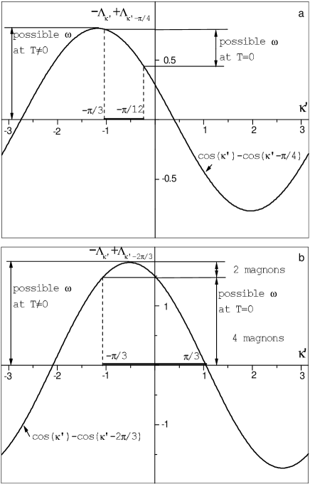
Figure 7: $-\Lambda_{\kappa^{\prime}}+\Lambda_{\kappa^{\prime}-\kappa}$ versus $\kappa^{\prime}$ for the non-random chain with $J_{0}=-1$, $\Omega_{0}=0.5$. a) $\kappa=\frac{\pi}{4}$; b) $\kappa=\frac{2\pi}{3}$.

Let us turn to the discussion of the obtained results. At first let us consider a non-random case (formulae (10) - (12), Fig. 5). To explain the observed frequency profiles one must take into account the fact that they reflect the dynamic properties of the magnetic chain conditioned by the exciting of two magnons with energies $\Lambda_{{\kappa}^{\prime}}=\Omega_{0}+J_{0}\cos\kappa^{\prime}$ and $\Lambda_{{\kappa}^{\prime\prime}}=\Omega_{0}+J_{0}\cos\kappa^{\prime\prime}$ for which $\omega=-\Lambda_{{\kappa}^{\prime}}+\Lambda_{{\kappa}^{\prime\prime}}$ and $\kappa^{\prime\prime}={\kappa}^{\prime}-{\kappa}$. Besides, at $T=0$ ($\beta\to\infty$) the magnon energies must have the corresponding signs due to the Fermi factors involved into (10), namely $\Lambda_{{\kappa}^{\prime}}<0$, $\Lambda_{{\kappa}^{\prime\prime}}>0$. Consider, for example, $S_{zz}(\frac{\pi}{4},\omega)$ for $\Omega_{0}=0.5$ (the curve for $\kappa=\frac{\pi}{4}$ in Fig. 5c and the dashed curve in Fig. 6b). Since $\Lambda_{\kappa}=0.5-\cos\kappa$ for $T=0$, because of the Fermi factors, $\kappa^{\prime}$ may vary only from $-\frac{\pi}{3}$ to $-\frac{\pi}{12}$ and, hence, $\kappa^{\prime}-\frac{\pi}{4}$ varies from $-\frac{7\pi}{12}$ to $-\frac{\pi}{3}$, whereas for non-zero temperature $\kappa^{\prime}$ varies from $-\pi$ to $\pi$. The value of $-\Lambda_{\kappa^{\prime}}+\Lambda_{\kappa^{\prime}-\frac{\pi}{4}}=-2\sin{\frac{\pi}{8}}\sin{\left(\kappa^{\prime}-\frac{\pi}{8}\right)}$ is shown in Fig. 7a. Evidently, at $T=0$, the lower frequency at which the non-zero value of $S_{zz}(\frac{\pi}{4},\omega)$ appears, $\omega_{l}$, is equal to $\cos{\frac{\pi}{12}}-\cos{\frac{\pi}{3}}=0.46592\ldots$ and the upper frequency $\omega_{u}$, after which $S_{zz}(\frac{\pi}{4},\omega)$ disappears, is equal to $\cos{\frac{\pi}{3}}-\cos{\frac{7\pi}{12}}=0.75881\ldots\;$; for non-zero temperature $\omega_{l}=0$ and $\omega_{u}=2\sin\frac{\pi}{8}=0.76536\ldots$ (see Fig. 7a). The value of $S_{zz}(\frac{\pi}{4},\omega)$ is determined by the value of the slope of the curve depicted in Fig. 7a and this explains why $S_{zz}(\frac{\pi}{4},\omega_{l})<S_{zz}(\frac{\pi}{4},\omega_{u})$ at $T=0$, as well as why $S_{zz}(\frac{\pi}{4},\omega_{u})\to\infty$ at non-zero temperature. Note that, as it can be seen from Fig. 7a, the value of $S_{zz}(\frac{\pi}{4},\omega)$ is determined by two pairs of magnons that satisfy the conditions $\omega=-\Lambda_{{\kappa}^{\prime}}+\Lambda_{{\kappa}^{\prime\prime}}$ and $\kappa^{\prime\prime}={\kappa}^{\prime}-{\kappa}$, however, at $T=0$, because of the additional requirement $\Lambda_{{\kappa}^{\prime}}<0$, $\Lambda_{{\kappa}^{\prime\prime}}>0$, only one pair of magnons can contribute to $S_{zz}(\frac{\pi}{4},\omega)$.

Consider further, for example, $S_{zz}(\frac{2\pi}{3},\omega)$ for $\Omega_{0}=0.5$ (the curve for $\kappa=\frac{2\pi}{3}$ in Fig. 5c and the dashed curve in Fig. 6d). For $T=0$, $\kappa^{\prime}$ may vary only from $-\frac{\pi}{3}$ to $\frac{\pi}{3}$, whereas for non-zero temperature $\kappa^{\prime}$ varies from $-\pi$ to $\pi$. The value of $-\Lambda_{\kappa^{\prime}}+\Lambda_{\kappa^{\prime}-\frac{2\pi}{3}}=-\sqrt{3}\sin\left(\kappa^{\prime}-\frac{\pi}{3}\right)$ is shown in Fig. 7b. As it can be seen from this figure, for $T=0$, as well as for non-zero temperature $\omega_{l}=0$ and $\omega_{u}=\sqrt{3}=1.73205\ldots\;$. Besides, $S_{zz}(\frac{2\pi}{3},\omega_{u})\to\infty$ for any temperature. The abrupt change in $S_{zz}(\frac{2\pi}{3},\omega)$ at $T=0$ at $\omega=1.5$ is due to the fact that for lower frequencies only one pair of magnons, because of the Fermi factors, contributes to $S_{zz}(\frac{2\pi}{3},\omega)$, whereas for higher frequencies two pairs of magnons are involved in forming $S_{zz}(\frac{2\pi}{3},\omega)$. At non-zero temperature $S_{zz}(\frac{2\pi}{3},\omega)$ is always conditioned by two pairs of magnons.

Let us pass to random models (formula (9), Fig. 6). For such models the transverse dynamic structure factor is again conditioned by two magnons $\Lambda_{p}$ and $\Lambda_{q}$, for which $\omega=-\Lambda_{p}+\Lambda_{q}$ and the quantity

$$\Delta(\kappa,p,q)=\sum_{n=0,\pm 1,\pm 2,\ldots}{\mbox{e}}^{{\mbox{i}}\kappa n}g_{pj}g_{p,j+n}g_{qj}g_{q,j+n}$$

has a non-zero value. Besides, at $T=0$, $\Lambda_{p}<0$, $\Lambda_{q}>0$. Apparently, there is no simple rigorous explanation for the behaviour of the random-averaged frequency profiles depicted in Fig. 6. However, it is easy to note that the kind of naive reasoning presented below does work for such a case. Consider at first the case $\kappa=\frac{\pi}{4}$ at low temperature. As it was shown above, the non-zero value of $S_{zz}(\frac{\pi}{4},\omega_{l})$ in a non-random case was conditioned by two magnons with the energies $0.5-\cos\frac{\pi}{12}=-0.46592\ldots$ and $0.5-\cos\frac{\pi}{3}=0$, respectively. As it can be seen in Fig. 8, where the random-averaged densities of magnon states $\overline{\rho(E)}=\overline{\frac{1}{N}\sum_{k=1}^{N}\delta(E-\Lambda_{k})}$ obtained from (5) are depicted, such a pair of “magnons” does exsist for $a=-1.01$ (Fig. 8a) and does not exsist for $a=1.01$ (Fig. 8b) or for the case of a non-correlated disorder (Fig. 8c). This observation is in agreement with the changes in the frequency profile due to different types of disorder shown in Fig. 6b (compare the curves 1, 4 and 2, 3 at $\omega_{l}$). In the non-random case the non-zero value of $S_{zz}(\frac{\pi}{4},\omega_{u})$ was conditioned by two magnons with the energies $0.5-\cos\frac{\pi}{3}=0$ and $0.5-\cos\frac{7\pi}{12}=0.75881\ldots\;$, respectively. From Fig. 8 one can see that the density of states for such magnons is diminished because of the disorder that agrees with the changes in $S_{zz}(\frac{\pi}{4},\omega_{u})$ shown in Fig. 6b.

Consider further the case $\kappa=\frac{2\pi}{3}$ at low temperature. For the non-random case $S_{zz}(\frac{2\pi}{3},\omega_{l})$ arises due to two magnons $\Lambda_{\frac{\pi}{3}}$ and $\Lambda_{-\frac{\pi}{3}}$ with the zero energy. As it can be seen in Fig. 8, the disorder affects the density of states at $E=0$ for $a=1.01$ and the non-correlated disorder more than for $a=-1.01$ that agrees with the changes in the frequency profile (Fig. 6d). $S_{zz}(\frac{2\pi}{3},\omega_{u})$ is formed by two magnons with the energies $0.5-\cos\frac{\pi}{6}=-0.36602\ldots$ and $0.5-\cos\frac{5\pi}{6}=1.36602\ldots\;$, respectively. The density of magnon states for such energies is more diminished for the non-correlated disorder (Fig. 8c) than for the correlated one (Figs. 8a, 8b) which agrees with the smaller value of $\overline{S_{zz}(\frac{2\pi}{3},\omega_{u})}$ in the former case in comparison with the latter.

To summarize, we extended the consideration of the spin-$\frac{1}{2}$ isotropic $XY$ chain with a correlated Lorentzian disorder presented in Ref. 14, examining numerically the dynamics of transverse spin correlations. We obtained the frequency dependences of the transverse dynamic structure factor at different values of the wave vector and temperature. We found the possible influences of the correlated disorder on the frequency profiles of the transverse dynamic structure factor. Within certain frequency regions the introducing of the correlated disorder may yield almost no changes in the value of $\overline{S_{zz}(\kappa,\omega)}$, whereas the non-correlated disorder always erodes the frequency profiles of $\overline{S_{zz}(\kappa,\omega)}$. The studied possible influences of the correlated disorder on the dynamic properties may be useful for the analysis of experimental data obtained in dynamic experiments for quasi-one-dimensional spin-$\frac{1}{2}$ isotropic $XY$ compounds.

The authors are grateful to Prof. M. Shovgenyuk for providing the possibility to perform the numerical calculations. The paper was discussed at Magdeburg University and Dortmund University. O. D. is grateful to Prof. J. Richter and Prof. J. Stolze for their warm hospitality. He is also indebted to Mrs. Olga Syska for the financial support.

List of figure captions

FIG. 1. Time dependence of the transverse spin correlation functions $r_{j,j+n}(t)={\mbox{Re}}\left[\langle s_{j}^{z}(t)s_{j+n}^{z}\rangle\right.$ $\left.-\langle s_{j}^{z}\rangle\langle s_{j+n}^{z}\rangle\right]$ for $J_{0}=-1$, $\Omega_{0}=0.5$, $\Gamma=0$ at $\beta=1000$. a) $N=150$, $j=j+n=75$; b) $N=300$, $j=j+n=150$; c) $N=300$, $j=150$, $j+n=250$. In this figure and in Figs. 2, 4 we plotted only the real parts of correlation functions since their imaginary parts exhibit qualitatively the same behaviour.

FIG. 2. Time dependence of $R_{\kappa}^{n^{\star}}(t)={\mbox{Re}}\sum_{n=0,\pm 1,\ldots,\pm n^{\star}}{\mbox{e}}^{{\mbox{i}}\kappa n}\left[\langle s_{150}^{z}(t)s_{150+n}^{z}\rangle-\langle s_{150}^{z}\rangle\langle s_{150+n}^{z}\rangle\right],$ $\kappa=\pi$ for $J_{0}=-1$, $\Omega_{0}=0.5$, $\Gamma=0$, $N=300$ at $\beta=1000$ for $n^{\star}=50$ (a) and $n^{\star}=100$ (b).

FIG. 3. $S_{zz}(\kappa,\omega)$ at $\kappa=\frac{\pi}{8}$ (1), $\kappa=\frac{\pi}{4}$ (2), $\kappa=\frac{2\pi}{3}$ (3), $\kappa=\frac{3\pi}{4}$ (4), $\kappa=\pi$ (5) for the uniform chain with $J_{0}=-1$, $\Omega_{0}=0.5$ at $\beta=1000$: exact results (11), (12) (dashed curves) versus numerical ones (solid curves). a) $N=280$, $j=140$, $n^{\star}=100$, $t_{c}=200$, $\epsilon=0.01$; b) $N=1800$, $j=900$, $n^{\star}=800$, $t_{c}=1200$, $\epsilon=0.01$; c) $N=1800$, $j=900$, $n^{\star}=800$, $t_{c}=1200$, $\epsilon=0.005$.

FIG. 4. Time dependence of $\overline{R_{\kappa}^{n^{\star}}(t)},$ $\kappa=\pi$ for $J_{0}=-1$, $\Omega_{0}=0.5$, $\Gamma=0.1$, $a=1.01$, $N=300$, $n^{\star}=100$ at $\beta=1000$; the random-averaged quantity comes as the result of averaging over 1000 realizations (a), 11000 realizations (b), and 21000 realizations (c).

FIG. 5. Frequency dependence of the transverse dynamic structure factor (11), (12) for $J_{0}=-1$ and different values of transverse field $\Omega_{0}=0$ (a), $\Omega_{0}=0.25$ (b), $\Omega_{0}=0.5$ (c), $\Omega_{0}=0.75$ (d), $\Omega_{0}=0.99$ (e) at different values of wave vector $\kappa=\frac{\pi}{8},\frac{\pi}{4},\frac{\pi}{2},\frac{2\pi}{3},\frac{3\pi}{4},\pi$ (from left to right) at $\beta=1000$. At high temperatures the frequency profiles of $S_{zz}(\kappa,\omega)$ are the same for all values of $\Omega_{0}$ (f).

FIG. 6. Frequency dependence of the random-averaged transverse dynamic structure factor (8) at different values of wave vector $\kappa=\frac{\pi}{8}$ (a), $\kappa=\frac{\pi}{4}$ (b), $\kappa=\frac{\pi}{2}$ (c), $\kappa=\frac{2\pi}{3}$ (d), $\kappa=\frac{3\pi}{4}$ (e), $\kappa=\pi$ (f) for model (1) with $J_{0}=-1,$ $\Omega_{0}=0.5,$ $\Gamma=0.1$ at $\beta=1000.$ 1) correlated disorder (3) with $a=-1.01;$ 2) correlated disorder (3) with $a=1.01;$ 3) independent exchange couplings and transverse fields, the latter are distributed according to probability distribution (4) with $|a|\Gamma=0.101;$ 4) non-random case $\Gamma=0$ (dashed curves).

FIG. 7. $-\Lambda_{\kappa^{\prime}}+\Lambda_{\kappa^{\prime}-\kappa}$ versus $\kappa^{\prime}$ for the non-random chain with $J_{0}=-1$, $\Omega_{0}=0.5$. a) $\kappa=\frac{\pi}{4}$; b) $\kappa=\frac{2\pi}{3}$.

FIG. 8. Density of states $\overline{\rho(E)}$ for model (1) with $J_{0}=-1,$ $\Omega_{0}=0.5,$ $\Gamma=0.1.$ a) correlated disorder (3) with $\Gamma=0.1,$ $a=-1.01$; b) correlated disorder (3) with $\Gamma=0.1,$ $a=1.01$; c) independent exchange couplings (2) with $\Gamma=0.1$ and transverse fields (4) with $|a|\Gamma=0.101$; the density of states for the non-random case $\Gamma=0$ is depicted by dashed curves.

Figure 1: Time dependence of the transverse spin correlation functions $r_{j,j+n}(t)={\mbox{Re}}\left[\langle s_{j}^{z}(t)s_{j+n}^{z}\rangle\right.$ $\left.-\langle s_{j}^{z}\rangle\langle s_{j+n}^{z}\rangle\right]$ for $J_{0}=-1$, $\Omega_{0}=0.5$, $\Gamma=0$ at $\beta=1000$. a) $N=150$, $j=j+n=75$; b) $N=300$, $j=j+n=150$; c) $N=300$, $j=150$, $j+n=250$. In this figure and in Figs. 2, 4 we plotted only the real parts of correlation functions since their imaginary parts exhibit qualitatively the same behaviour.

Figure 2: Time dependence of $R_{\kappa}^{n^{\star}}(t)={\mbox{Re}}\sum_{n=0,\pm 1,\ldots,\pm n^{\star}}{\mbox{e}}^{{\mbox{i}}\kappa n}\left[\langle s_{150}^{z}(t)s_{150+n}^{z}\rangle-\langle s_{150}^{z}\rangle\langle s_{150+n}^{z}\rangle\right],$ $\kappa=\pi$ for $J_{0}=-1$, $\Omega_{0}=0.5$, $\Gamma=0$, $N=300$ at $\beta=1000$ for $n^{\star}=50$ (a) and $n^{\star}=100$ (b).

Figure 3: $S_{zz}(\kappa,\omega)$ at $\kappa=\frac{\pi}{8}$ (1), $\kappa=\frac{\pi}{4}$ (2), $\kappa=\frac{2\pi}{3}$ (3), $\kappa=\frac{3\pi}{4}$ (4), $\kappa=\pi$ (5) for the uniform chain with $J_{0}=-1$, $\Omega_{0}=0.5$ at $\beta=1000$: exact results (11), (12) (dashed curves) versus numerical ones (solid curves). a) $N=280$, $j=140$, $n^{\star}=100$, $t_{c}=200$, $\epsilon=0.01$; b) $N=1800$, $j=900$, $n^{\star}=800$, $t_{c}=1200$, $\epsilon=0.01$; c) $N=1800$, $j=900$, $n^{\star}=800$, $t_{c}=1200$, $\epsilon=0.005$.

Figure 4: Time dependence of $\overline{R_{\kappa}^{n^{\star}}(t)},$ $\kappa=\pi$ for $J_{0}=-1$, $\Omega_{0}=0.5$, $\Gamma=0.1$, $a=1.01$, $N=300$, $n^{\star}=100$ at $\beta=1000$; the random-averaged quantity comes as the result of averaging over 1000 realizations (a), 11000 realizations (b), and 21000 realizations (c).

Figure 5: Frequency dependence of the transverse dynamic structure factor (11), (12) for $J_{0}=-1$ and different values of transverse field $\Omega_{0}=0$ (a), $\Omega_{0}=0.25$ (b), $\Omega_{0}=0.5$ (c), $\Omega_{0}=0.75$ (d), $\Omega_{0}=0.99$ (e) at different values of wave vector $\kappa=\frac{\pi}{8},\frac{\pi}{4},\frac{\pi}{2},\frac{2\pi}{3},\frac{3\pi}{4},\pi$ (from left to right) at $\beta=1000$. At high temperatures the frequency profiles of $S_{zz}(\kappa,\omega)$ are the same for all values of $\Omega_{0}$ (f).

Figure 6: Frequency dependence of the random-averaged transverse dynamic structure factor (8) at different values of wave vector $\kappa=\frac{\pi}{8}$ (a), $\kappa=\frac{\pi}{4}$ (b), $\kappa=\frac{\pi}{2}$ (c), $\kappa=\frac{2\pi}{3}$ (d), $\kappa=\frac{3\pi}{4}$ (e), $\kappa=\pi$ (f) for model (1) with $J_{0}=-1,$ $\Omega_{0}=0.5,$ $\Gamma=0.1$ at $\beta=1000.$ 1) correlated disorder (3) with $a=-1.01;$ 2) correlated disorder (3) with $a=1.01;$ 3) independent exchange couplings and transverse fields, the latter are distributed according to probability distribution (4) with $|a|\Gamma=0.101;$ 4) non-random case $\Gamma=0$ (dashed curves).

Figure 8: Density of states $\overline{\rho(E)}$ for model (1) with $J_{0}=-1,$ $\Omega_{0}=0.5,$ $\Gamma=0.1.$ a) correlated disorder (3) with $\Gamma=0.1,$ $a=-1.01$; b) correlated disorder (3) with $\Gamma=0.1,$ $a=1.01$; c) independent exchange couplings (2) with $\Gamma=0.1$ and transverse fields (4) with $|a|\Gamma=0.101$; the density of states for the non-random case $\Gamma=0$ is depicted by dashed curves.

References

[1]
E. R. Smith,
J. Phys. C 3, 1419 (1970).
[2]
E. Barouch and B. M. McCoy,
Stud. Appl. Math. 51, 57 (1972).
[3]
R. O. Zaitsev,
Zh. Eksp. Teor. Fiz. 63, 1487 (1972)
(in Russian).
[4]
F. Matsubara and S. Katsura,
Prog. Theor. Phys. 49, 367 (1973).
[5]
E. Barouch and I. Oppenheim,
Physica 76, 410 (1974).
[6]
H. Braeter and J. M. Kowalski,
Physica A 87, 243 (1977).
[7]
H. Nishimori,
Phys. Lett. A 100, 239 (1984).
[8]
D. S. Fisher,
Phys. Rev. Lett. 69, 534 (1992);
D. S. Fisher,
Phys. Rev. B 51, 6411 (1995).
[9]
H. Asakawa,
Physica A 233, 39 (1996).
[10]
A. P. Young and H. Rieger,
Phys. Rev. B 53, 8486 (1996);
A. P. Young,
Phys. Rev. B 56, 11691 (1997).
[11]
R. H. McKenzie,
Phys. Rev. Lett. 77, 4804 (1996).
[12]
P. Henelius and S. M. Girvin,
Phys. Rev. B 57, 11457 (1998).
[13]
J. Hermisson,
cond-mat/9808238.
[14]
O. Derzhko and J. Richter,
Phys. Rev. B 55, 14298 (1997).
[15]
W. John and J. Schreiber,
Phys. Status Solidi B 66, 193 (1974);
J. Richter,
Phys. Status Solidi B 87, K89 (1978);
K. Handrich and S. Kobe,
Amorphe Ferro- und Ferrimagnetica,
Academie-Verlag, Berlin, 1980 (in German).
[16]
L. L. Gonçalves and A. P. Vieira,
J. Magn. Magn. Mater. 177-181, 79 (1998).
[17]
O. Derzhko and T. Krokhmalskii,
J. Phys. Stud. (Lviv) 2, 263 (1998).
[18]
O. Derzhko and T. Krokhmalskii,
Ferroelectrics 153, 55 (1994);
192, 21 (1997);
O. Derzhko, T. Krokhmalskii, and T. Verkholyak,
J. Magn. Magn. Mater. 157/158, 421 (1996);
O. Derzhko and T. Krokhmalskii,
Phys. Rev. B 56, 11659 (1997);
O. Derzhko and T. Krokhmalskii,
Phys. Status Solidi B 208, 221 (1998).
[19]
G. A. Farias and L. L. Gonçalves,
Phys. Status Solidi B 139, 315 (1987).
[20]
J. Stolze, A. Nöppert, and G. Müller,
Phys. Rev. B 52, 4319 (1995).
[21]
M. D’Iorio, R. L. Armstrong, and D. R. Taylor,
Phys. Rev. B 27, 1664 (1983);
M. D’Iorio, U. Glaus, and E. Stoll,
Solid State Commun. 47, 313 (1983).
[22]
In our numerical calculations we put
and
.
[23]
Formula (9) can be also used
for the numerical calculation of the transverse
dynamic structure factor.
[24]
S. Katsura, T. Horiguchi, and M. Suzuki,
Physica 46, 67 (1970).
[25]
H. A. Gersch,
Phys. Rev. B 1, 2270 (1970).
[26]
T. N. Tommet and D. L. Huber,
Phys. Rev. B 11, 450 (1975).
[27]
V. S. Viswanath, G. Müller,
The recursion method.
Application to many-body dynamics,
Springer-Verlag, Berlin, Heidelberg, 1994.