State Orthogonalization by Building a Hilbert Space: A New Approach to Electronic Quantum Transport in Molecular Wires

Abstract

Quantum descriptions of many complex systems are formulated most naturally in bases of states that are not mutually orthogonal. We introduce a general and powerful yet simple approach that facilitates solving such models exactly by embedding the non-orthogonal states in a new Hilbert space in which they are by definition mutually orthogonal. This novel approach is applied to electronic transport in molecular quantum wires and is used to predict conductance antiresonances of a new type that arise solely out of the non-orthogonality of the local orbitals on different sites of the wire.

PACS: 03.65.-w, 73.61.Ph, 73.50.-h

The predictions of quantum mechanics that relate to observable phenomena do not depend on the particular basis that is selected to represent state vectors in Hilbert space. However choosing a basis of states whose physical significance is clear and that are mutually orthogonal can be extremely helpful in theoretical work. Bases constructed from the eigenstates of a set of commuting operators that represent physical observables have both of these desirable properties[1]. But for complex systems that are composed of simpler building blocks, it is tempting to use the eigenstates of the Hamiltonians of the separate building blocks as basis states even though such bases are not orthogonal. In solid state physics and quantum chemistry where the building blocks are atoms, each with its own electronic eigenstates, this choice of basis gives rise to the widely used tight-binding[2] and Hückel[3] models. An analogous approach that models nucleons as bags of quarks[4] is used in theoretical work on nuclei and nuclear matter.[5] The representations of the Hilbert spaces of complex systems that are obtained in this way are intuitively appealing but the non-orthogonality has been a significant drawback. Standard orthogonalization schemes such as Gram-Schmidt do not help here because they are unwieldy for large systems and do not preserve the atomistic character of the basis states. Wannier functions[2] provide orthogonalized local basis states for perfect periodic structures, but they have the disadvantage of not being eigenstates of atomic Hamiltonians and also have no analog for disordered solids, liquids or molecules. Löwdin functions[6] do not require a periodic lattice but they too are not eigenstates of atomic Hamiltonians and do not have a simple physical interpretation. Thus, rather than working with nonorthogonal bases,[7] it has been customary in much of the literature, for the sake of simplicity, to neglect the overlaps between the non-orthogonal states, as is done in LCAO (linear combination of atomic orbitals) models of electronic structure, tight-binding theories of Anderson localization in disordered systems, and Hubbard and t-J models of electronic correlations. However, non-orthogonality can have non-trivial physical implications. For example, it is closely related to gauge interactions and fractional exclusion statistics, as has been pointed out by Haldane[8]. Better ways to treat it are therefore of interest.

In this Letter we introduce a simple, powerful and general method that facilitates obtaining exact solutions of quantum problems in which the non-orthogonality of the basis is important. Our approach is to build a new Hilbert space around the non-orthogonal basis states, a space in which these states are by definition orthogonal, and to work in this new Hilbert space. We demonstrate the power, simplicity and flexibility of this novel approach by applying it to electronic quantum transport in molecular wires and predicting that these should exhibit conductance antiresonances of a new type. These antiresonances are a direct and surprising physical consequence of the non-orthogonality of the electronic orbitals on different atoms of the wire, which is included naturally in our theory.

A molecular wire is a single molecule connecting a pair of metallic contacts. Such devices have recently begun to be realized experimentally and their electrical conductances are being measured.[9, 10, 11, 12] Electron transport in molecular wires has been studied theoretically by considering the transmission probability for electrons to scatter through the structure.[10, 13, 14, 15, 16, 17] As with other mesoscopic systems, the electrical conductance $G$ of the molecule is related to the transmission probability $T$ at the Fermi level by the Landauer formula $G={\frac{e^{2}}{h}}T$.[18] Molecular wires display a number of interesting transport phenomena, one of which is transmission antiresonances.[19, 20, 21, 14] Antiresonances are zeroes of the transmission $T$ and correspond to electrons being perfectly reflected by the molecule. They also occur in semiconductor systems.[22] An analytic theory of molecular antiresonances was first proposed by Ratner[19] in the context of electron transfer between donor and acceptor sites of a molecule, but his treatment did not include the effects of the non-orthogonality of the atomic states. The present approach yields an analytic description of molecular wire transport (including antiresonances) that treats this non-orthogonality exactly and permits us to explore its physical implications.

Our starting point is the Schrödinger equation

$$H|\Psi\rangle=E|\Psi\rangle$$ (1)

where the Hamiltonian operator $H$ and eigenvector $|\Psi\rangle$ are defined in a Hilbert space $A$. We wish to solve Eq.(1) for $|\Psi\rangle$ which is expressed as $|\Psi\rangle=\sum_{n}\Psi_{n}|n\rangle$ in a non-orthogonal basis $\{|n\rangle\}$ of Hilbert space $A$. In this basis Eq.(1) takes the form

$$\sum_{n}H_{m,n}\Psi_{n}=E\sum_{n}S_{m,n}\Psi_{n}$$ (2)

where $H_{m,n}=\langle m|H|n\rangle$ and $S_{m,n}=\langle m|n\rangle$ is the overlap matrix.[23] Let us rewrite Eq.(2) as

$$\sum_{n}H^{E}_{m,n}\Psi_{n}=E\Psi_{m}$$ (3)

where

$$H^{E}_{m,n}=H_{m,n}-E(S_{m,n}-\delta_{m,n}).$$ (4)

Eq.(3) can be viewed as the matrix form of the Schrödinger equation

$$H^{E}|\Psi^{\prime}\rangle=E|\Psi^{\prime}\rangle$$ (5)

where $H^{E}$ and $|\Psi^{\prime}\rangle$ are a new Hamiltonian operator and its eigenvector defined in a new Hilbert space $A^{\prime}$ [24] in which the basis states $\{|n\rangle\}$ are orthonormal with $\langle m|n\rangle=\delta_{m,n}\,$, $|\Psi^{\prime}\rangle=\sum_{n}\Psi_{n}|n\rangle$ has the same coefficients $\Psi_{n}$ as $|\Psi\rangle$, and the new Hamiltonian operator is defined by its matrix elements through $\langle m|H^{E}|n\rangle=H^{E}_{m,n}$. According to Eq.(4), $H^{E}$ is Hermitian in $A^{\prime}$ because $E$ is real and $H_{m,n}\,$, $S_{m,n}$ and $\delta_{m,n}$ are Hermitian matrices.

Thus we have transformed a problem that was formulated in terms of a nonorthogonal basis into an equivalent one in an orthogonal basis in a different Hilbert space. Other orthogonalization schemes (such as that of Löwdin [6]) differ from ours in this as well as other respects.[25]

It should be noted that only the eigenvectors of $H^{E}$ that have the eigenvalue $E$ have the same coefficients $\Psi_{n}$ as eigenvectors of the true Hamiltonian $H$. The other eigenvectors of $H^{E}$ do not correspond to any eigenstate of the physical Hamiltonian $H$, but they never the less play an important role when calculating the Green’s function corresponding to $H^{E}$.

Since no assumptions at all have been made about the nature of the system being considered, this method of orthogonalization by switching to a new Hilbert space is extremely general. If the basis states $\{|n\rangle\}$ are tight binding atomic orbitals, then the present transformation (unlike the transformation to Wannier functions) can be used irrespective of the types of atoms involved or their locations in space. Furthermore, our transformation has the additional flexibility that the non-orthogonal basis states need not all be of the same generic type. For example, some of them may be atomic orbitals and others molecular orbitals on some cluster(s) of atoms that form a part of the physical system. This flexibility will be exploited below. We now proceed to outline the application to molecular wire quantum transport.

We begin by solving analytically an idealized model of a molecular wire consisting of a molecule attached to two identical semi-infinite single-channel leads which are represented by 1D chains of atoms. For this system we find it convenient to choose a non-orthogonal basis consisting of atomic orbitals $\{|n\rangle\}$ with $n=-\infty\dots-1$ on the left lead and $n=1\dots\infty$ on the right lead and molecular orbitals (MO’s) $\{|j\rangle\}$ for the molecule. In terms of this basis we write electron eigenstates $|\Psi\rangle$ of $H$ in which the electron is incident on the molecule from the left lead and transmitted with probability $T$ through the molecule to the right lead as

$$|\Psi\rangle = \sum_{n=-\infty}^{-1}\Psi_{n}|n\rangle+\sum_{n=1}^{\infty}\Psi_{n}|n\rangle+\sum_{j}c_{j}|j\rangle$$ (6)

The transmission probability $T$ that enters the Landauer electrical conductance of the wire is given by $T=|\Psi_{1}|^{2}$. Solving for $\Psi_{1}$ analytically in the nonorthogonal basis is difficult so we transform to the new Hilbert space $A^{\prime}$ where the solution is more straightforward. As we have already shown, the coefficients $\Psi_{n}$ remain the same in $A^{\prime}$ where the basis $\{|n\rangle,|j\rangle\}$ is orthogonal, so that the above expression for $T$ is valid in either Hilbert space.

We evaluate $\Psi_{1}$ by solving a Lippmann-Schwinger (LS) equation that describes electron scattering in the molecular wire. We define this LS equation in the new Hilbert space $A^{\prime}$ where it takes the form

$$|\Psi^{\prime}\rangle=|\Phi^{\prime}\rangle+G^{\prime}(E)W^{E}|\Psi^{\prime}\rangle.$$ (7)

Here $|\Psi^{\prime}\rangle$ is the eigenstate of the transformed Hamiltonian $H^{E}$ whose coefficients correspond to those of the untransformed scattering eigenstate $|\Psi\rangle$ defined above Eq.(6). $W^{E}$ is defined by separating $H^{E}$ into two parts, $H^{E}=H_{o}^{E}+W^{E}$, where the matrix elements of $H_{o}^{E}$ between lead orbitals $\{|n\rangle\}$ and MO’s $\{|j\rangle\}$ all vanish in the space $A^{\prime}$ and $W^{E}$ couples the molecule to the adjacent lead sites. $|\Phi^{\prime}\rangle$ is an eigenstate of $H_{0}^{E}$ with eigenvalue $E$ that is confined to the left lead. $G^{\prime}(E)=(E-H_{0}^{E})^{-1}$ is the Green’s function of the decoupled system.

The validity of the LS Eq.(7) depends crucially on the clear distinction between states on the leads and those on the molecule that can only be made in Hilbert space $A^{\prime}$; non-orthogonality leads to contradictions if analogs of the entities that enter (7) are constructed in $A$. The transformation to $A^{\prime}$ also introduces energy dependent hopping into the transformed Hamiltonian as prescribed in Eq. (4). The energy dependence of the coupling $W^{E}$ between the molecule and leads in Hilbert space $A^{\prime}$ will be important in the determination of antiresonances. Our choice of a set of MO’s $\{|j\rangle\}$ that are mutually orthogonal in $A$ means that the Green’s function for the isolated molecule is formally unaffected by our transformation. This choice allows a simpler evaluation of the molecular Green’s function that enters $G^{\prime}(E)$. An atomic orbital basis set non-orthogonal in $A$ could be chosen instead, however the solution would then be less transparent.

The evaluation of the Green’s function $G^{\prime}(E)$ and solution of the LS equation (7) in the orthogonal basis $\{|n\rangle,|j\rangle\}$ of Hilbert space $A^{\prime}$ is straightforward and will be presented in detail elsewhere. Here we will focus on the salient results for molecular wire conductance antiresonances and their physical significance. We find

$$\Psi_{1}=\frac{P\Phi^{\prime}_{-1}}{[(1-Q)(1-R)-PS]}$$ (8)

where

$$P = G^{\prime}_{1,1}\sum_{j}W^{E}_{1,j}G^{\prime}_{j}W^{E}_{j,-1}$$

$$Q = G^{\prime}_{1,1}\sum_{j}(W^{E}_{1,j})^{2}G^{\prime}_{j}$$

$$R = G^{\prime}_{1,1}\sum_{j}(W^{E}_{-1,j})^{2}G^{\prime}_{j}$$

$$S = G^{\prime}_{1,1}\sum_{j}W^{E}_{-1,j}G^{\prime}_{j}W^{E}_{j,1}$$

The sum over $j$ is over only the MO’s. In the above, $W^{E}_{1,j}=H_{1,j}-ES_{1,j}$ is the energy-dependent hopping element of $H^{E}$ between the first lead site and the $j^{th}$ MO in terms of the hopping element of the original Hamiltonian $H$ and the overlap in the non-orthogonal basis. The Green’s function on the molecule is expanded in terms of its molecular eigenstates (which, as mentioned above, are unchanged by the transformation) and this gives $G^{\prime}_{j}=1/(E-\epsilon_{j})$ for the $j^{th}$ MO with energy $\epsilon_{j}$. $G^{\prime}_{1,1}$ is the diagonal matrix element of the Green’s function $G^{\prime}(E)$ at the end site of the isolated lead.

Conductance antiresonances of the molecular wire occur where the transmission $T=|\Psi_{1}|^{2}$ is equal to zero. From Eq. (8) this happens when $P=0$, i.e., at Fermi energies E that are the roots of

$$\sum_{j}\frac{(H_{1,j}-ES_{1,j})(H_{j,-1}-ES_{j,-1})}{E-\epsilon_{j}}=0.$$ (9)

Two distinct mechanisms for antiresonances in molecular wire transport can be identified from Eq. (9):

In the first of these mechanisms, antiresonances arise due to an interference between molecular states that may differ in energy, as is seen directly from Eq. (9): An electron incident from the left lead, hops from the lead site adjacent to the molecule onto each of the MO’s with a weight $W^{E}_{j,-1}$. It propagates through each of the different orbitals $j$ and hops onto the right lead with a weight $W^{E}_{1,j}\,.$ These processes interfere with each other and where they cancel (9) is satisfied and an antiresonance occurs. This is in essence the same interference mechanism as has been identified previously in work on electron transfer between molecular donor and acceptor sites and, in the absence of the overlaps $S_{1,j}$ and $S_{j,-1}$, our result (9) agrees with that obtained there.[19]

The second antiresonance mechanism, which has no analog in previous work, arises solely from the nonorthogonality of atomic orbitals that we have included in our analytic theory with the help of the Hilbert space transformation. It occurs when only a single MO $k$ couples appreciably to the leads. In such cases, Eq. (9) becomes $(H_{k,-1}-ES_{k,-1})(H_{1,k}-ES_{1,k})=0$. Two antiresonances are possible in this case. They occur at energies $E$ where a matrix element of the transformed Hamiltonian ${\bf H}^{E}={\bf H}-E({\bf S-1})$ that is responsible for hopping between the molecule and one of the leads vanishes in the new Hilbert space. Thus the non-orthogonality of two orbitals can actually prevent electron hopping between these orbitals from taking place, blocking electron transmission along the wire and creating an antiresonance. This is a counterintuitive effect since one would normally expect orbital overlap to aid electron transfer between the orbitals rather than hinder it. It underscores the importance of including the effects of nonorthogonality fully in tight-binding theories.

The above analytic theory of antiresonances was developed for an idealized molecular wire model with semi-infinite single channel leads. We now compare these analytic results with numerical calculations for a more realistic molecular wire model. The system we consider consists of (100) Au leads bonded to a molecule as shown in the inset to Fig. 1. It is representative of a class of current experimental devices which use a mechanically controlled break junction to form a pair of nanoscale metallic contacts which are then bridged by a single molecule, the molecular wire.[9] The molecular wire we consider consists of two “chain” segments and an “active” segment. The purpose of the chains is to reduce the many propagating electron modes in the metallic contacts down to a single mode which propagates along the chains. Thus the (finite) chains supplant the 1D ideal leads of our analytic model. We model this molecular wire and its bonding to the 3D metallic contacts by using extended Hückel to calculate the hopping elements and overlaps between the non-orthogonal atomic orbitals that make up this system. It is the interaction between the non-orthogonal orbitals on the chains and the active segment that generates the antiresonances. Each chain consists of 7 C-H groups and is terminated with a sulphur atom which bonds to a gold lead. For the energies of interest (near the Fermi level of gold) these chains only support a single $\pi$ mode. We chose an arbitrary active molecular segment with two $\pi$-like MO’s which only interact with the $\pi$ mode of the chains. The active segment is considered to be long enough that there is no direct coupling between the chains, as in our analytic theory. Fig. 1 shows a plot of the contact-to-contact transmission calculated numerically for this model. The arrows indicate the locations of the antiresonances predicted by our analytic model (i.e., Eq. (9)) using the same model parameters. The agreement is very good; two antiresonances are found in each case at -10.2 eV and -10.4 eV, close to the Fermi energy of the gold leads. The transmission does not drop exactly to zero since in this calculation second nearest neighbor interactions are also included. The experimental signature is a drop in the differential conductance of the molecular wire. The agreement between Eq. (9) and Fig. 1 indicates that our analytic result derived for the idealized molecular wire model using the new approach to take account of non-orthogonality has predictive power for more complex systems.

In conclusion: Many of the quantum problems that arise in physics and chemistry are formulated most naturally in a basis of states that are not mutually orthogonal. In this Letter we have shown that the exact solution of such problems is greatly facilitated by embedding these non-orthogonal basis states in a new Hilbert space in which they are by definition mutually orthogonal but the matrix elements of the Hamiltonian are energy-dependent. The power, simplicity and flexibility of this novel approach was illustrated by applying it to analytic and numerical calculations of electronic quantum transport in molecular wires. A new mechanism for molecular wire conductance antiresonances was identified which arises solely out of the non-orthogonality of local orbitals on different sites of the wire.

We would like to thank H. Trottier for rewarding discussions. This work was supported by NSERC.

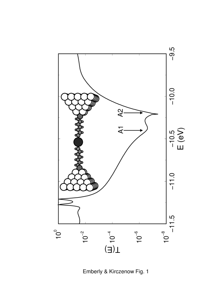
FIG. 1.: Electronic transmission probability $T$ calculated numerically for molecular wire shown in inset. Antiresonance is predicted at A1 and A2 by the analytic condition (9). The active molecule has two $\pi$ levels with energies $\epsilon_{a}=-13.0$ eV and $\epsilon_{b}=-9.0$ eV. The coupling and overlap of these two levels to the left (L) and right (R) chain molecules are $W_{L,a}=-5.0$ eV, $W_{L,b}=-2.5$ eV, $S_{L,a}=0.3$, $S_{L,b}=0.2$ and $W_{R,a}=-2.7$ eV, $W_{R,b}=-1.8$ eV, $S_{R,a}=0.25$, $S_{R,b}=0.15$.

REFERENCES

- [1] P. A. M. Dirac, The Principles of Quantum Mechanics, ch. III, 4th ed., Oxford University Press, 1958.
- [2] J. M. Ziman, Principles of the Theory of Solids, 2nd ed., Cambridge University Press, 1972.
- [3] R. J. Hoffmann, J. Chem. Phys. 39, 1397 (1963).
- [4] W. A. Bardeen et al., Phys. Rev. D 11, 1094 (1975); A. Chodos et al., Phys. Rev. D 9, 3471 (1974).
- [5] For a review see A. W. Thomas, Adv. Nucl. Phys. 13, 1 (1984).
- [6] P. O. Löwdin, J. Chem. Phys. 18, 365 (1950).
- [7] See P. Fulde, Electron Correlations in Molecules and Solids, 3rd ed., ch. 2, Springer-Verlag, Berlin, 1995.
- [8] F. D. M. Haldane, Phys. Rev. Lett. 67, 939 (1991).
- [9] M. A. Reed, C. Zhou, C. J. Muller, T. P. Burgin, and J. M Tour, Science 278, 252 (1997).
- [10] S. Datta, W. Tian, S. Hong, R. Reifenberger, J. I. Henderson, C. P. Kubiak, Phys. Rev. Lett. 79, 2530 (1997).
- [11] R. P. Andres, J. D. Bielefeld, J. I. Henderson, D. B. Janes, V. R. Kolagunta, C. P. Kubiak, W. J. Mahoney, and R. G. Osifchin, Science 273, 1690 (1996).
- [12] L. A. Bumm, J. J. Arnold, M. T. Cygan, T. D. Dunbar, T. P. Burgin, L. Jones II, D. L. Allara, J. M. Tour, P. S. Weiss, Science 271, 1705 (1996).
- [13] M. P. Samanta, W. Tian, S. Datta, J. I. Henderson, and C. P. Kubiak, Phys. Rev. B 53, R7626 (1996).
- [14] M. Kemp, A. Roitberg, V. Mujica, T. Wanta and M. A. Ratner, J. Phys. Chem 100, 8349 (1996).
- [15] C. Joachim, and J. F. Vinuesa, Europhys. Lett. 33, 635 (1996).
- [16] V. Mujica, M. Kemp, A. Roitberg and M. Ratner, J. Chem. Phys. 104, 7296 (1997).
- [17] E. Emberly and G. Kirczenow, Phys. Rev. B (1998).
- [18] R. Landauer, IBM J. Res. Dev. 1, 223 (1957); R. Landauer, Phys. Lett. 85A, 91 (1981).
- [19] M. A. Ratner, J. Phys. Chem. 94, 4877 (1990).
- [20] J. M. Lopez-Castillo, A. Filali-Mouhim, J. P. Jay-Gerin, J. Phys. Chem. 97, 9266 (1993).
- [21] A. Cheong, A. E. Roitberg, V. Mujica, and M. A. Ratner, J. Photochem. Photobiol. A: Chem. 82, 81 (1994).
- [22] F. Sols et al., Appl. Phys. Lett. 54, 350 (1989); S. Datta, Superlatt. Microstruct. 6, 83 (1989). Z.-L. Ji and K.-F. Berggren, Phys. Rev. B 45, 6652 (1992). T. B. Boykin, B. Pezeshki, and J. S. Harris, Jr., Phys. Rev. B 46, 12769 (1992). E. Tekman and P. F. Bagwell, Phys. Rev. B. 48, 2553 (1993). P. J. Price, Phys. Rev. B 48, 17301 (1993). Z. Shao, W. Porod, and C. S. Lent, Phys. Rev. B 49, 7453 (1994). R. Akis, P. Vasilopoulos, and P. Debray, Phys. Rev. B 52, 2805(1995).
- [23] If the basis is incomplete, Eq. (2) may be understood variationally. See, for example, Ref.[6].
- [24] Let be the vector space spanned by the basis vectors , in which . The new Hilbert space is the completion of with respect to the norm topology.
- [25] Löwdin’s orthogonalized basis states are constructed as linear combinations of non-orthogonal states in the same Hilbert space.[6] By contrast, we construct an orthogonal basis by embedding non-orthogonal states in a different Hilbert space in which they are by definition orthogonal. The transformed Hamiltonian that arises naturally in our formalism also differs from that of Löwdin which in the present notation is . The energy-dependent hopping that appears in is the physical mechanism of the novel molecular wire antiresonances that are predicted in this Letter.