Interfacial Velocity Corrections due to Multiplicative Noise

Abstract

The problem of velocity selection for reaction fronts has been intensively investigated, leading to the successful marginal stability approach for propagation into an unstable state. Because the front velocity is controlled by the leading edge which perforce has low density, it is interesting to study the role that finite particle number fluctuations have on this picture. Here, we use the well-known mapping of discrete Markov processes to stochastic differential equations and focus on the front velocity in the simple $A+A\stackrel{{\scriptstyle\leftarrow}}{{\rightarrow}}A$ system. Our results are consistent with a recent (heuristic) proposal that $v_{MS}-v\sim{1\over\ln^{2}{N}}$.

I Introduction

There has been a great deal of interest in the problem of reaction front propagation in non-equilibrium systems. This issue arises in systems ranging from flames [1] to bacterial colonies [2], from solidification patterns [3] to genetics [4]. Most of the theoretical work in this area involves solving deterministic reaction-diffusion equations. Here, we focus on effects that occur when one goes beyond this mean-field treatment and considers the effects of fluctuations.

By now, it is clear that there are several possible mechanisms whereby the velocity of a deterministic reaction-diffusion front can be selected. For cases where we propagate into a linearly unstable state, the marginal stability criterion [5] suggests that the fastest stable front is the one that is observed for all physical initial conditions. For propagation into a metastable state, there is a unique front solution consistent with the boundary conditions and hence there is no selection to be done. In between, there is the case of a nonlinearly unstable state in which the exponentially localized front is chosen. These principles have been verified in many examples and in some cases can be rigorously derived [6].

However, it is understood that deterministic equations are often only approximations to the actual non-equilibrium dynamics. This is particularly clear in the case of chemical reaction systems where the true dynamics is a continuous time Markov process which gives rise to a reaction-diffusion equation only in the limit of an infinite number of particles per site [7]. More generally, having a finite number of particles gives rise to fluctuations that may be important in the front propagation problem. It has been hypothesized in a variety of systems [8, 9, 10] that the leading effect of such fluctuations is to provide an effective cutoff on the reaction rate at very chemical concentrations. If this is the case, calculations by Brunet and Derrida [11] predict that in the case of a system which (in the deterministic limit) exhibits (linear) marginal stability (MS) selection , the front velocity obeys the scaling $v_{MS}-v\sim{1\over\ln^{2}{N}}$, where $N$ is the (mean-field) number of particles per site in the stable state. Direct simulations of the underlying Markov processes have, in two cases to date [11, 12], been consistent with this predicted form, albeit with some uncertainty regarding the coefficient. Also, we note in passing that the cutoff idea is the simplest one which explains the recently discovered fact[13] that one can have diffusive instabilities of a front in a chemical reaction system which do not show up in a reaction-diffusion treatment thereof.

Our purpose here is to introduce a different approach for studying the role of these fluctuations in modifying the front velocity. There is a well-established machinery which transforms the master equation for Markov processes for chemical reaction systems to the solution of an associated stochastic differential equation. This was first proposed by Doi[14], and clarified in some seminal work of Peliti [15]. This framework has in fact been used for the study of critical phenomena associated with bulk transitions in reaction dynamics [16], but has not been applied to the issue of front propagation far from such a bulk transition. Here, we directly simulate the relevant stochastic equation; this requires the analytic solution of a (interesting in its own right) single-site problem, which then, via a split-step method, allows up to time-step the entire spatially-extended system. Our results to date verify the Brunet-Derrida scaling and in fact are even consistent with the coefficient obtained by the cutoff approach.

The outline of this work is as follows. In section II, we review the mapping from the master equation to a Langevin equation with multiplicative noise. Next, we solve a variety of single-site problems as a prelude to introducing our simulation method. We then tackle the front problem numerically and compare our findings to the results obtained by augmenting the deterministic system with a cutoff. In order to accomplish this, the findings of Brunet and Derrida are extended to include the effects of finite resolution in space and time. At the end, we summarize the open issues that we hope to address in the future.

II Derivation of the stochastic equation

In this paper, we will study the following space-lattice reaction scheme:

$$A\stackrel{{\scriptstyle\alpha}}{{\rightarrow}}2A$$ (1)

$$2A\stackrel{{\scriptstyle\beta}}{{\rightarrow}}A$$ (2)

$$A\stackrel{{\scriptstyle\lambda}}{{\rightarrow}}0$$ (3)

$$0\stackrel{{\scriptstyle\tau}}{{\rightarrow}}A$$ (4)

$$A_{i}\stackrel{{\scriptstyle\mu}}{{\rightarrow}}A_{e}$$ (5)

where $e$ is the nearest neighbor sites of site $i$; $\alpha$, $\beta$, $\lambda$, $\mu$, $\tau$ are rates of the corresponding reactions, i.e. probabilities of transition per unit time. This process is described by the master equation

$$\frac{dP(\{n_{i}\};t)}{dt}=\sum_{i}\left[\frac{\partial P(\{n_{i}\};t)}{\partial t}\bigg{|}_{\alpha}+\frac{\partial P(\{n_{i}\};t)}{\partial t}\bigg{|}_{\beta}+\frac{\partial P(\{n_{i}\};t)}{\partial t}\bigg{|}_{\lambda}\right.+$$ (6)

$$\left.\frac{\partial P(\{n_{i}\};t)}{\partial t}\bigg{|}_{\tau}+\frac{\partial P(\{n_{i}\};t)}{\partial t}\bigg{|}_{\mu}\right]$$ (7)

which states that the probability $P(\{n_{i}\};t)$ of having $n_{i}$ particles on sites $i$ at some time $t$ changes via each of the elementary processes:

1. one particle splitting into two

   $$\frac{\partial P(\{n_{i}\};t)}{\partial t}\bigg{|}_{\alpha}=\alpha[(n_{i}-1)P(\ldots,n_{i}-1,\ldots;t)-n_{i}P(\ldots,n_{i},\ldots;t)]$$ (8)

2. two particle reaction with one being annihilated

   $$\frac{\partial P(\{n_{i}\};t)}{\partial t}\bigg{|}_{\beta}=\beta[(n_{i}+1)n_{i}P(\ldots,n_{i}+1,\ldots;t)-n_{i}(n_{i}-1)P(\ldots,n_{i},\ldots;t)]$$ (9)

3. one particle annihilation

   $$\frac{\partial P(\{n_{i}\};t)}{\partial t}\bigg{|}_{\lambda}=\lambda[(n_{i}+1)P(\ldots,n_{i}+1,\ldots;t)-n_{i}P(\ldots,n_{i},\ldots;t)]$$ (10)

4. particle birth from vacuum

   $$\frac{\partial P(\{n_{i}\};t)}{\partial t}\bigg{|}_{\tau}=\tau[P(\ldots,n_{i}-1,\ldots;t)-P(\ldots,n_{i},\ldots;t)]$$ (11)

5. diffusion

   $$\frac{\partial P(\{n_{i}\};t)}{\partial t}\bigg{|}_{\mu}=\mu\sum_{e}[(n_{e}+1)P(\ldots,n_{i}-1,n_{e}+1,\ldots;t)-n_{i}P(\ldots,n_{i},\ldots;t)]$$ (12)

In this section, we provide a self-contained derivation of the stochastic equation whose solution is directly related to the solution of this master equation. This is by now fairly standard, but we find it useful to include this derivation here both for completeness and for fixing various parameters in the final Langevin system.

Following Doi[14], we introduce a vector in Fock space $|\{n_{i}\}\rangle$ and raising and lowering operators $\hat{a}^{+}_{i}$, $\hat{a}_{i}$ with the properties:

$$\hat{a}_{i}|\ldots,n_{i},\ldots\rangle=n_{i}|\ldots,n_{i}-1,\ldots\rangle$$ (13)

$$\hat{a}_{i}^{+}|\ldots,n_{i},\ldots\rangle=|\ldots,n_{i}+1,\ldots\rangle$$ (14)

and the commutation relation

$$[\hat{a}_{i},\hat{a}_{j}^{+}]=\delta_{ij}$$ (15)

We choose an initial condition for the master equation $(\ref{master})$ to be a Poisson state,

$$P(\{n_{i}\};t=0)=e^{-N_{A}(0)}\prod_{i}\frac{n_{0i}^{n_{i}}}{n_{i}!}$$ (16)

where $N_{A}(0)=\sum\limits_{i}n_{0i}$ is the expected total number of particles. If we define the time dependent vector

$$|\phi(t)\rangle=\sum_{\{n_{i}\}}P(\{n_{i}\};t)|\{n_{i}\}\rangle$$ (17)

the master equation can be written in the Schrödinger form

$$\frac{\partial}{\partial t}|\phi(t)\rangle=-\hat{H}|\phi(t)\rangle$$ (18)

where $\hat{H}=\sum_{i}\hat{H}_{i}$ and the latter is given by

$$-\mu\sum_{e}\hat{a}_{i}^{+}(\hat{a}_{e}-\hat{a}_{i})+\alpha[1-\hat{a}_{i}^{+}]\hat{a}_{i}^{+}a_{i}-\beta[1-\hat{a}_{i}^{+}]\hat{a}_{i}^{+}\hat{a}_{i}^{2}-\lambda[1-\hat{a}_{i}^{+}]\hat{a}_{i}+\tau[1-\hat{a}_{i}^{+}]$$ (19)

The formal solution of this equation is

$$|\phi(t)\rangle=e^{-\hat{H}t}|\phi(0)\rangle=e^{-N_{A}(0)}e^{-\hat{H}t}e^{\sum_{i}\hat{a}_{i}^{+}n_{0i}}|0\rangle$$ (20)

To be able to calculate average values for observables, we need to introduce the projection state

$$\langle|=\langle 0|\prod_{i}e^{\hat{a}_{i}}$$ (21)

The external product of this with any state $|\{n_{i}\}\rangle$ gives $1$. Then any normal-ordered polynomial operator satisfies

$$\langle|Q(\{\hat{a}_{i}^{+}\},\{\hat{a}_{i}\})=\langle|Q(\{1\},\{\hat{a}_{i}\})$$ (22)

Using this equation we get for any observable

$$\langle A(t)\rangle=\sum_{\{n_{i}\}}A(\{n_{i}\})P(\{n_{i}\};t)=\langle|\tilde{A}(\{\hat{a}_{i}\})|\phi(t)\rangle$$ (23)

where $\tilde{A}(\{\hat{a}_{i}\})$ is what we obtain by using the commutation relation to normal order $A$ and thereafter setting $\hat{a}_{i}^{+}$ to $1$.

In order to write a path integral representation for the time evolution operator, we introduce a set of coherent states ( see [17] for more strict treatment)

$$\|\{z_{i}\}\rangle=e^{\sum_{i}z_{i}\hat{a}_{i}^{+}-z_{i}}|0\rangle$$ (24)

where $z_{i}$ is complex eigenvalue of $\hat{a}_{i}$. In the case of real positive $\{z_{i}\}$ this states are Poissonian states with $\langle{n}_{i}\rangle=z_{i}$. By inserting the completeness relation,

$$1=(\prod_{i}\int\frac{d^{2}z_{i}}{\pi}e^{-|z_{i}|^{2}+z_{i}+z_{i}^{*}})\|z\rangle\langle z\|$$ (25)

where $d^{2}z_{i}=d(Re{}z_{i})d(Im{}z_{i})$, into expression $(\ref{avr})$ we get

$$\langle|\tilde{A}(\{\hat{a}_{i}\})e^{-\hat{H}t}|\phi(0)\rangle=\langle|\tilde{A}(\{\hat{a}_{i}\})(1-\hat{H}\Delta t)^{N\Delta t}\|z^{(0)}\rangle=$$ (26)

$$\langle|\tilde{A}(\{\hat{a}_{i}\})(\prod_{i}\int\frac{d^{2}z^{(N)}_{i}}{\pi}e^{-|z_{i}^{(N)}|^{2}+z_{i}^{(N)}+{z^{*}_{i}}^{(N)}})\|z^{(N)}\rangle\langle z^{(N)}\|\times$$ (27)

$$(\prod_{j=1}^{N}(1-\hat{H}\Delta t))\|z^{(0)}\rangle=\langle 0|(\prod_{j=1}^{N}\prod_{i}\int\frac{d^{2}z^{(j)}_{i}}{\pi})\tilde{A}(\{z^{(N)}_{i}\})e^{-S}|0\rangle$$ (28)

where $\Delta t=t/N$, $|\phi(0)\rangle=\|z^{(0)}\rangle$ and

$$S=\sum_{j=1}^{N}\sum_{i}(H_{i}({z^{*}}^{(j)},z^{(j-1)})\Delta t+|z_{i}^{(j)}|^{2}-{z_{i}^{*}}^{(j)}z_{i}^{(j-1)}-z_{i}^{(N)}+z_{i}^{(0)})=$$ (29)

$$\sum_{j=0}^{N-1}\sum_{i}\Delta t(\frac{\bar{z}_{i}^{(j+1)}(z_{i}^{(j+1)}-z_{i}^{(j)})}{\Delta t}+H_{i}(\bar{z}^{(j+1)}+1,z^{(j)}))$$ (30)

Here ${z_{i}^{*}}^{(j)}=\bar{z}_{i}^{(j)}+1$ and $H_{i}(\{{z_{i}^{*}}^{(j+1)}\},\{z^{(j)}\})$ is the same function of ${z_{i}^{*}}^{(j+1)}$, ${z_{i}^{*}}^{(j)}$ as $\hat{H}_{i}(\{\hat{a}_{i}^{+}\},\{\hat{a}_{i}\})$ of $\hat{a}_{i}^{+}$, $\hat{a}_{i}$. In the continuous time limit we get

$$\langle A(t_{0})\rangle=\frac{\int\prod_{i}{\cal D}\bar{z}_{i}{\cal D}z_{i}A(\{z_{i}(t_{0})\})e^{-S[\{\bar{z}_{i}(t)\},\{z_{i}(t)\};t_{0}]}}{\int\prod_{i}{\cal D}\bar{z}_{i}{\cal D}z_{i}e^{-S[\{\bar{z}_{i}(t)\},\{z_{i}(t)\};t_{0}]}}$$ (31)

with

$$S[\{\bar{z}_{i}(t)\},\{z_{i}(t)\};t_{0}]=\sum_{i}\int_{0}^{t_{0}}dt\ \left(\bar{z}_{i}(t)[\frac{d}{dt}-\mu\nabla^{2}]z_{i}(t)-\alpha(1+\bar{z}_{i}(t))\bar{z}_{i}(t)z_{i}(t)+\right.$$ (32)

$$\left.\beta(1+\bar{z}_{i}(t))\bar{z}_{i}(t)z_{i}^{2}(t)+\lambda\bar{z}_{i}(t)z_{i}(t)-\tau\bar{z}_{i}(t)\right)$$ (33)

where $\nabla^{2}$ is the lattice Laplacian $z_{i}(t)=\sum_{e}(z_{e}(t)-z_{i}(t))$. Now, we linearize the action using the Stratonovich transformation

$$e^{\bar{z}_{i}^{2}(\alpha z_{i}-\beta z_{i}^{2})dt}\sim\int d\eta_{i}e^{-\frac{1}{2}\eta_{i}^{2}-\bar{z}_{i}\sqrt{2(\alpha z_{i}-\beta z_{i}^{2})}\eta_{i}\sqrt{dt}}$$ (34)

and integrate out the $\bar{z}$ variables

$$\langle A(t_{0})\rangle\sim\int\prod_{i}{\cal D}\eta_{i}{\cal D}z_{i}e^{-\frac{1}{2}\sum_{i}\int_{0}^{t_{0}}dt\eta_{i}^{2}(t)}A(\{z_{i}(t_{0})\})\prod_{t=0}^{t_{0}}\delta(dz_{i}(t)-\mu\nabla^{2}z_{i}(t)dt-$$ (35)

$$\alpha z_{i}(t)dt+\beta z_{i}^{2}(t)dt+\lambda z_{i}(t)dt-\tau dt-\sqrt{2(\alpha z_{i}(t)-\beta z_{i}^{2}(t))}\eta_{i}(t)\sqrt{dt})$$ (36)

In this expression, there are $\delta$-functions at every time; this means that only $z_{i}(t)$ which satisfy to the Langevin equation

$$dz_{i}(t)=\mu\nabla^{2}z_{i}(t)dt+(\alpha-\lambda)z_{i}(t)dt-\beta z_{i}^{2}(t)dt+\tau dt+\sqrt{2(\alpha z_{i}(t)-\beta z_{i}^{2}(t))}dW_{i}(t)$$ (37)

(where $W_{i}(t)$ is a Wiener process) contribute to the path integral. In other words, the variables $z_{i}(t)$ remain on the trajectories described by equation $(\ref{Langevin})$. Note that this equation must be considered as an Ito stochastic differential equation, since we can see from the form of the action $(\ref{daction})$ that the updating the variables $z_{i}$ to time-step $j+1$ only requires knowledge of the variables at time-step $j$. Also, we note that for $\lambda\geq 0$ and for small enough (positive) $\tau$, if the initial conditions specify $0\leq z_{i}(0)\leq\alpha/\beta$, this will remain true for all subsequent time. Thus, equation $(\ref{Langevin})$ describes the temporal evolution of the system as sequence of Poissonian states [18].

For further analysis, we rescale $(\ref{Langevin})$ with $z=u\alpha/\beta$, $t\rightarrow t/\alpha$, $\tilde{\lambda}=\lambda/\alpha$, $\tilde{\tau}=\tau\beta/\alpha^{2}$, and $\tilde{\mu}=\mu/\alpha$. If we furthermore let $N=\alpha/\beta$ be the mean-field number of particles in the presence only the first two processes (no spontaneous decay or spontaneous creation), we obtain

$$du_{i}=\tilde{\mu}\nabla^{2}u_{i}dt+(1-\tilde{\lambda})u_{i}dt-u_{i}^{2}dt+\tilde{\tau}dt+\sqrt{\frac{2}{N}}\sqrt{u_{i}-u_{i}^{2}}dW_{i}$$ (38)

with initial conditions $0\leq u_{i}(0)\leq 1$.

III Exact Solutions of Some Local Langevin Equations

In the absence of process $(\ref{birth})$, i.e. at $\tau=0$, equation $(\ref{L})$ has an absorbing state $u=0$. In the vicinity of this point, equation $(\ref{L})$ cannot be treated by merely setting $dt$ to a finite time-step. Such a scheme would often give rise to a negative $u$, due to the (very-large) noise term. One ad-hoc way to circumvent this difficulty was given by Dickman [19], who proposed to re-introduce discreteness into the state-space in the vicinity of the absorbing state. Although this approach appears to work (it seems to lead to the correct critical behavior near the bulk transition of this class of models), it seems to be a step backward; after all, the original process was discrete and the whole purpose of using the Langevin formalism is to provide a (hopefully more analytically tractable) continuum description. But, one must then come up with a different scheme for updating the stochastic variables.

Our approach is to solve exactly the stochastic part of the evolution equation and embed this via the split-step method in a complete update scheme for a finite time-step $\Delta t$. We will discuss the details of this scheme in the next section. Here, we provide an analytic solution for several (local) Langevin equations, as these results will be needed later. Also, this solution set is of interest on its own. There is some limited consideration of equations of this sort in the literature [20], but as far as we can determine, these explicit solutions for the case of physical no-flux boundary conditions at the absorbing state has not previously appeared.

So, we consider Langevin equations with just the noise term. Let us start with the simplest example,

$$du=\sqrt{2u}dW$$ (39)

The probability density $P(u,t)$ satisfies the associated Fokker-Planck equation

$$\frac{\partial P(u,t)}{\partial t}=\frac{\partial^{2}}{\partial u^{2}}uP(u,t)$$ (40)

with initial condition $P(u,t)\bigg{|}_{t=t_{in}}=\delta(u-u_{0})$. We want our solution to be equal to zero at $u<0$ and have no flux leaking out of this point; this will guarantee that the total probability remains a constant, which we will choose to be unity.

To solve this equation, we define $\psi=uP$ and Laplace transform in time to obtain

$$u\frac{\partial^{2}\tilde{\psi}}{\partial u^{2}}(s)\ -\ s\tilde{\psi}(s)\ =\ u_{0}\delta(u-u_{0})$$ (41)

Here, $\tilde{\psi}(s)$ is the transform of $\psi$. If we let $y=2\sqrt{u}$, this can be written as

$$\left(\frac{\partial^{2}}{\partial y^{2}}-\frac{1}{y}\frac{\partial}{\partial y}-s\right)\tilde{\psi}\ =\ -\frac{y_{0}}{2}\delta(y-y_{0})$$ (42)

The homogeneous part of this equation can be recognized as a variant of Bessel’s equation. This allows us to write down a provisional solution in the form

$$\tilde{\psi}(s)\ =\ \frac{yy_{0}}{2}K_{1}(\sqrt{s}y_{>})I_{1}(\sqrt{s}y_{<})$$ (43)

where $I_{1}$ and $K_{1}$ are modified Bessel functions and $y_{>}(y_{<})$ is the larger (smaller) of $y$ and $y_{0}$. Returning to the original variables,

$$\tilde{P}(s)\ =\ 2\frac{\sqrt{u_{0}}}{\sqrt{u}}K_{1}(2\sqrt{su_{>}})I_{1}(2\sqrt{su_{<}})$$ (44)

This solution does not, of course, vanish for $u<0$ and hence we must modify it by multiplying by $\theta(u)$. This does not change the fact that it solves the equation away from $u=0$ but it does introduce a discontinuity of size $2\sqrt{u_{0}}K_{1}(2\sqrt{su_{0}})$. If we look at the original equation, we see that this leads to a $\delta$ function via $u\delta^{\prime}(u)=-\delta(u)$. This must be compensated by adding an explicit $\delta$ function piece to the solution. The final result is

$$\tilde{P}(s)\ =\ 2\frac{\sqrt{u_{0}}}{\sqrt{u}}K_{1}(2\sqrt{su_{>}})I_{1}(2\sqrt{su_{<}})\\ +\ 2\sqrt{\frac{u_{0}}{s}}K_{1}(2\sqrt{su_{0}})\delta(u)$$ (45)

We can do the inverse transform by the usual contour integral approach. The details are particularly unilluminating, so we merely quote the final result

$$P(u,t)\ =\ \frac{1}{t}\sqrt{\frac{u_{0}}{u}}e^{-(u+u_{0})/t}I_{1}(\frac{2\sqrt{uu_{0}}}{t})+e^{-u_{0}/t}\delta(u)$$ (46)

One can check explicitly that this solves the equation and also that $P$ remains normalized for all times. The $\delta$ function piece represents accumulation at the absorbing state; as $t$ gets large, all the probability end up there. The regular part of $P(u,t)$ is presented on the Figure 1. We see that as ratio $u_{0}/t$ becomes smaller, the distribution gradually shifts towards zero and differs from the Gaussian expected at very short times.

For completeness, we write down the solution of Langevin equations with additional terms. If we take the system,

$$du=\tau dt+\sqrt{2u}dW,$$ (47)

the probability density is

$$P(u,t)\ =\ \left(\frac{u_{0}}{u}\right)^{\frac{1-\tau}{2}}\ \frac{I_{\tau-1}(2\frac{\sqrt{uu_{0}}}{t})}{t}\ e^{-(u+u_{0})/t}$$ (48)

For this case, spontaneous birth from the vacuum prevents the system from falling irreversibly to the state $u=0$. Instead, there is an integrable power-law singularity near $u=0$ which becomes a $\delta$ function in the $\tau\rightarrow 0$ limit; this is shown in Figure 2.

For the system

$$du=\alpha udt+\sqrt{2u}dW$$ (49)

the probability density is

$$P(u,t)\ =\ e^{-\frac{\alpha u_{0}e^{\alpha t}}{e^{\alpha t}-1}}\delta(u)\ +\ \sqrt{g(t)\frac{u_{0}}{u}}I_{1}\left(2\sqrt{g(t)uu_{0}}\right)\ e^{-\alpha\frac{u+u_{0}e^{\alpha t}}{e^{\alpha t}-1}}$$ (50)

where $g(t)=\frac{\alpha^{2}e^{\alpha t}}{(e^{\alpha t}-1)^{2}}$. In this case, the drift toward infinity gives rise to a finite total probability (for long times) of falling into the absorbing state. One can also work out the case of both finite $\tau$ and finite $\alpha$.

For the system

$$du=\sqrt{2(u-u^{2})}dW$$ (51)

we can derive a series representation for the probability density,

$$P(u,t)=\sum_{m=1}^{+\infty}e^{-m(m+1)t}\frac{2m+1}{2m(m+1)}\sqrt{\frac{u_{0}(1-u_{0})}{u(1-u)}}P_{m}^{1}(2u_{0}-1)P_{m}^{1}(2u-1)+$$ (52)

$$\delta(u)[1-u_{0}-\sum_{m=1}^{+\infty}(-1)^{m}\frac{2m+1}{2m(m+1)}\sqrt{u_{0}(1-u_{0})}e^{-m(m+1)t}P_{m}^{1}(2u_{0}-1)]-$$ (53)

$$\delta(1-u)[u_{0}+\sum_{m=1}^{+\infty}\frac{2m+1}{2m(m+1)}\sqrt{u_{0}(1-u_{0})}e^{-m(m+1)t}P_{m}^{1}(2u_{0}-1)]$$ (54)

where $P_{m}^{1}(x)$ is Legendre polynomial. Successive terms in this sum decay rapidly because of the fast exponent, and the sum can be computed numerically to high accuracy. Note that there are absorbing states at both $u=0$ and $u=1$. If the initial state starts close to one of these, the probability is almost the same as $(\ref{solsqrt})$; if the initial state is in between, then for short times the system is almost Gaussian.

IV Front propagation

A Numerical method

We are interested in numerically solving equation $(\ref{Langevin})$, for the particular case of $\tau=\lambda=0$; this is case which reduces in the deterministic case to the well-studied Fisher equation[4] For this purpose, we define a function

$$F_{u_{0},\Delta t}(u)=\int_{0^{-}}^{u}P(u,\Delta t)du$$ (55)

where $P(u,\Delta t)$ is the analytical solution of a single-site Langevin equation such as $(\ref{L})$. This function has values ranging from $0$ to $1$. If $y$ is random variable homogeneously distributed on $[0,1]$, then $u=F^{-1}_{u_{0},\Delta t}(y)$ is distributed according to corresponding truncated Langevin equation at time $\Delta t$. The remaining parts of complete Langevin equation are deterministic and for those terms we can update $u$ via a simple Euler scheme. We then can combine this two steps together; we first compute the change in $u$ due to fluctuations and then the change of $u$ due to the deterministic part (using new value of $u$). Thus

$$u(t+\Delta t)=F^{-1}_{u(t),\Delta t}(y)+{\cal D}\{F^{-1}_{u(t),\Delta t}(y)\}\Delta t$$ (56)

where ${\cal D}\{u\}$ denotes the terms remaining after consideration of the noise term.

It is important to note that this scheme never allows the field to go below zero, but it does allow a variable to be stuck at zero until it is “lifted” by the diffusive interaction. This is an absolutely necessary aspect of simulating processes with an absorbing state. Approximations which do not allow for getting “stuck”, such as the system-size expansion method of Van-Kampen [7] (where the noise correlation is taken to be related to the solution of the deterministic limit of the equation) get this wrong and hence cannot get the correct front velocity. This explains why the simulation results of [21] do not at all exhibit the anomalous $N$ dependence expected via the Brunet-Derrida cutoff argument. As we will see, our approach is much more successful.

B Marginal stability criterion for a discretized Fisher equation

As $N$ gets large, our results should approach those of the deterministic system. Since this problem corresponds to propagation into an unstable region, the velocity should be given by the marginal stability approach. As is well known, this predicts a velocity equal to $2\sqrt{D}$, in the continuum (in time and space) limit. Here, we extend this result to a discrete lattice and a finite time update scheme, so as to be able to directly compare our simulation data with the theoretical expectation.

After linearization, the deterministic part of the discretized equation takes the form

$$\frac{u_{i}^{(j+1)}-u_{i}^{(j)}}{\Delta t}=\mu(u_{i+1}^{(j)}-2u_{i}^{(j)}+u_{i-1}^{(j)})+u_{i}^{(j)}$$ (57)

We want to compare this equation to the usual Fisher equation with diffusion coefficient $D$. This means that $\mu=D/h^{2}$; we will consider the case $D=1$. We assume that the front moves with constant velocity $c$ and therefore the variables $u_{i}^{(j)}$ show a stroboscopic picture of this motion at times $j\Delta t$ on the lattice sites $i$. If we move with the speed of the front we will see that its shape exponentially decays as $e^{q(ih-cj\Delta t)}$. Substitution of this expression to $(\ref{fd})$ gives the dependence of $c$ on the decay rate $q$

$$\frac{e^{-qc\Delta t}-1}{\Delta t}\ =\ \frac{2}{h^{2}}(\cosh qh-1)+1$$ (58)

The standard marginal stability argument predicts that we can determine the decay rate and asymptotic speed of the front (for a sufficiently localized initial state) by solving $(\ref{disp})$ as well its derivative with respect to $q$

$$ce^{-qc\Delta t}\ =\ -\frac{2}{h}\sinh qh$$ (59)

Simulations directly confirm this formula as well as the Brunet and Derrida [11] result (actually derived earlier by Bramson [22]) that $c_{\infty}-c(t)\sim 1/t$ (see Figures 3).

As already mentioned, it has been conjectured that the leading effect of the fluctuations is the imposition of an effective cutoff of order $1/N$ in the deterministic equation. To check this, we need to extend the Brunet and Derrida result to our discretized equation. The basic idea is that there must be a small imaginary part of the decay rate so at to satisfy the continuity conditions at the cutoff point; this is discussed in detail in [11]. This leads directly to

$$Im\ q\ =\ \frac{\pi q_{0}}{\ln(AN)}$$ (60)

where $q_{0}$ is solution from the marginal stability criterion and $A$ is some constant. Since $c^{\prime}(q)$ is zero at the marginal stability point, we can find the change in velocity $\delta c$ by considering the second derivative of the function $c(q)$ given by $(\ref{disp})$. We thus get

$$\delta c=\frac{\pi^{2}q_{0}(e^{-c_{0}q_{0}\Delta t}\cosh q_{0}h-\frac{c_{0}^{2}\Delta t}{2})}{\ln^{2}N}$$ (61)

Again, simulations confirm this formula (see Figure 4).

C Results

We now present the results of our simulation. We chose to make one further simplification. We use the pure square root noise term instead of the precisely correct term given in equation (38). We do this for computational ease, inasmuch as the expression derived for this case is much simpler than that of equation (52). Since it is only the effect of the noise near the $u=0$ absorbing state which is crucial for altering the selected velocity, this simplification should not be essential. Once we have done this, the resulting equation has the nice feature that the coefficient $1/\sqrt{N}$ in front of the noise term can be removed by the re-scaling $\hat{u}=uN$. This means that we can simulate equation (38) using a fixed probability table (with the same time step) for any $N$.

To actually evaluate the probability table $F_{u_{0},\Delta t}(u)$, we chose $512$ equidistant values of $\hat{u}_{0}$ in the interval from 0 to 30. For each $\hat{u}_{0}$, the interval of values for $\hat{u}$ where $F_{\hat{u}_{0},\Delta t=0.01}(\hat{u})$ is non-trivial was divided into $1024$ equidistant points. The new value of $\hat{u}$ was then determined by linear interpolation of the data from the table. For $\hat{u}_{0}>30$, new values of $\hat{u}$ were determined using a standard algorithm for the Gaussian distribution , since this distribution is the asymptotic limit of equation $(\ref{solsqrt})$, when $\hat{u}_{0}\gg\Delta t$, $\hat{u}\gg\Delta t$. The difference for this distribution and exact solution is small for $\hat{u}_{0}>30$. Finally, the computation of the stochastic term was turned off for $\hat{u}_{0}>10^{-3}N$. This should not affect the speed which, we have already argued, is only sensitive to what happens near $u=0$; this insensitivity was also checked directly by running some simulations in which the stochastic term is included for all values of $u$.

All of our simulations were run up to the time $t=10^{6}$. Four values of the velocity, corresponding to time intervals of approximately $2.x10^{5}$ were obtained so as to get an average and some error bar. In Figure 5. we show data in the form of $c-c_{\infty}$, where $c_{\infty}$ is calculated from equation (59), versus $\ln^{2}{N}$. Also plotted for comparison is the function $11/\ln^{2}{N}$. Note that over many orders of magnitude of $N$, the dependence derived by Brunet and Derrida provide a very good fit to the data.

To get a more accurate indication of the data for large $N$, we present in Figure 6 a series of three runs, for differing values of the spatial lattice spacing $h$. Under the hypothesis that the stochastic system should be precisely the same as the deterministic system with the cutoff added, the expected limiting values at infinite $N$ are shown as triangles on the axis. It is clearly impossible to definitively conclude that the curves are approaching these values. On the other hand, simple extrapolations come very close and we believe that it is more likely than not that this hypothesis is true. This is opposite to what was conjectured based on simulations of a discrete Markov process, where the velocity seems to scale albeit with a different coefficient. Given the incredibly slow convergence of this velocity at large $N$, we are pessimistic as to whether any purely simulational strategy would provide a definitive answer to this question. This therefore offers a crucial issue for future theoretical analysis to investigate.

V Summary

In this work, we have shown how to use the field-theoretic mapping of discrete Markov processes to stochastic equations for continuous density variable to address the role of finite-particle number fluctuations on the velocity of reaction fronts. Specifically, we studied a model which leads to the well-known Fisher equation in the $N\rightarrow\infty$ limit, where $N$ is the average number of particles per site in the stable state. Our goal is to understand how the usual marginal stability criterion becomes modified by these stochastic effects.

It is clear that having finite $N$ lowers the velocity at which a front (corresponding to the invasion of the unstable state by the stable one) will propagate. One attractive hypothesis is that the leading effect of the fluctuations is to to introduce an effect cutoff into the deterministic equation; this idea arose independently in model of biological evolution [9] and in mean field approaches for diffusion-limited-aggregation (DLA) [8]. Brunet and Derrida have shown that if this is the case, one should expect $v_{MS}-v={C\over\ln^{2}{N}}$, where $C=\pi^{2}$ for the case of continuous time and space. We have extended the calculation of $C$ to the finite lattice size, finite time-step system and compared this prediction with direct simulations of the relevant stochastic equation. Our results verify the form of the scaling and suggest that the coefficient may be correct as well.

One issue that is left unaddressed by our work to date concerns the effects of higher spatial dimensionality. It is likely, although unproven, that the velocity change will be smaller, as the fluctuations get averaged over the transverse directions. This seems to be the explanation for the findings of Riordan et al [23] that the reaction front looks mean-field like even for small $N$, in three and four dimensions. We hope to report on this issue in the future.

Finally, we point out yet again that there is no analytic treatment available for the velocity selection problem in the stochastic equation. Obvious expansion methods such as the system-size approach cannot work, as they neglect the essential role of the fluctuations to push the system back into the absorbing state at small density. We need to find a more powerful approach!

We thank D. Kessler for many useful discussions. We also acknowledge the support of the US NSF under grant DMR98-5735.

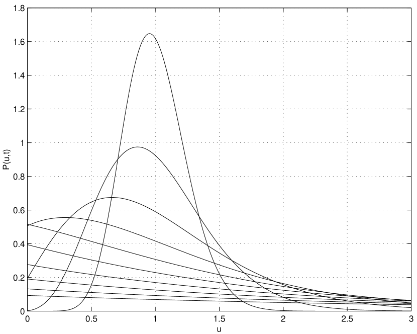
FIG. 1.: Function $(\ref{Lsqrt})$ with $u_{0}=1$ and $\Delta t=0.03(n^{2}-n+1)$ for $n=1,...,10$.

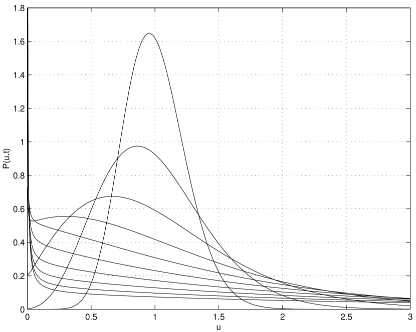
FIG. 2.: Function $(\ref{tau})$ with $u_{0}=1$ and $\Delta t=0.03(n^{2}-n+1)$ for $n=1,...,10$.

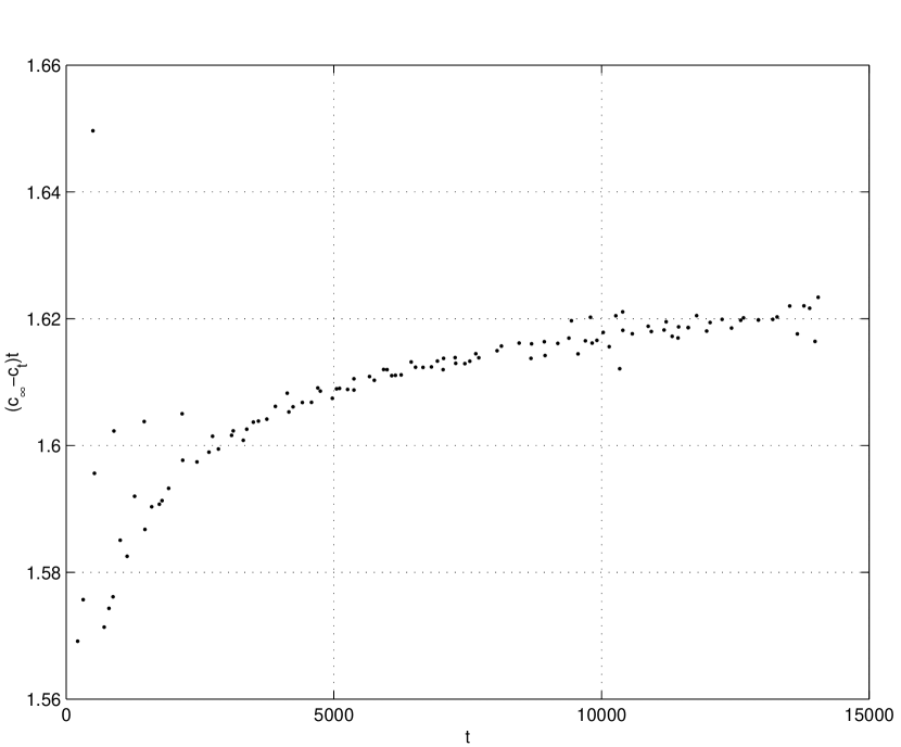
FIG. 3.: Front propagation for the discretized Fisher equation. Parameters were $\Delta t=0.01$, $h=1$; for this choice, equation $(\ref{fd})$ gives $c_{\infty}=2.054115884$. The speed is determined by registering every time some lattice point comes within some small interval around .5 and then merely using the ratio of the number per spaces moved over the time elapsed; this method leads to some scatter, as seen in the graph. Aside from showing agreement with the calculated $c_{\infty}$, the graph also shows how the system approaches the eventual $1/t$ in asymptotic behavior.

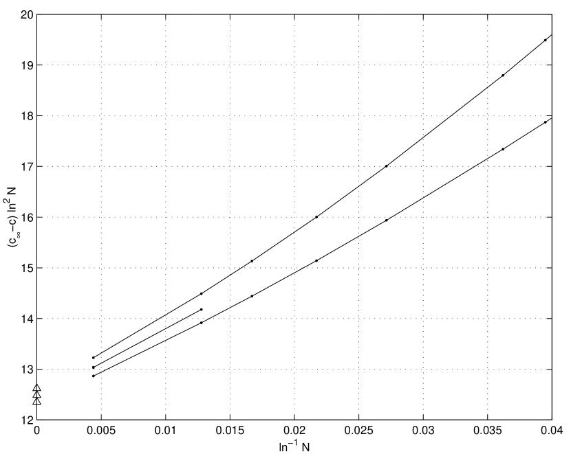
FIG. 4.: Dependence of the front speed on the deterministic cutoff. The curves represent simulation results calculated with the parameters $h=1$ and $\Delta t=0.01$; $0.015$; $0.02$ from top to bottom respectively. The cutoff was implemented via setting the field to zero at any time and place where it was below $1/N$. Points on $y$-axis represent theoretical values when $N\rightarrow\infty$ as given by equation $(\ref{delc})$.

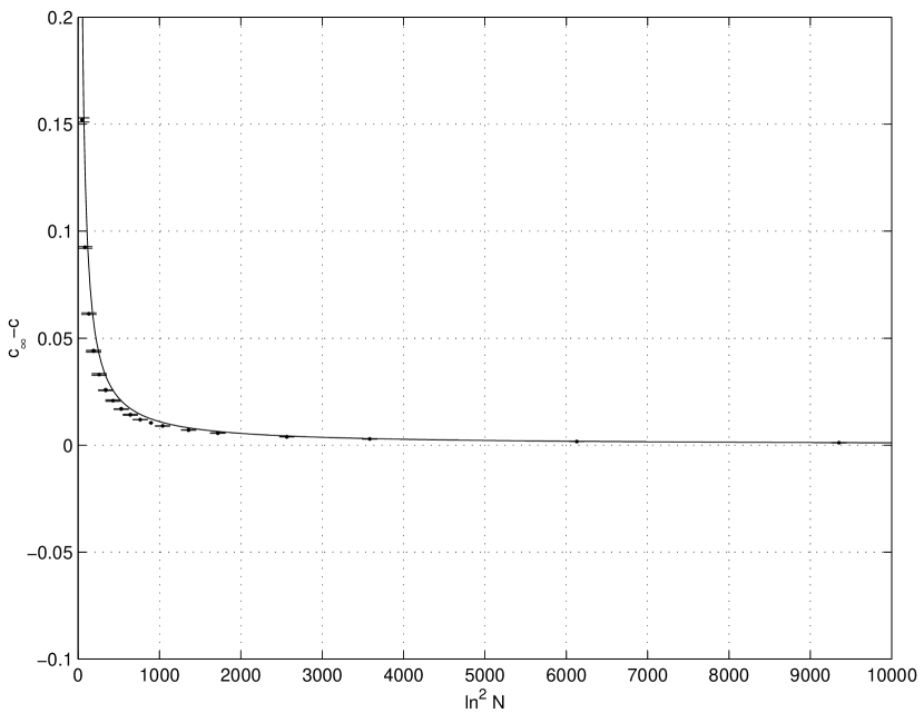
FIG. 5.: Front speed for the Langevin equation with parameters $\Delta t=0.01$ and $h=1$.

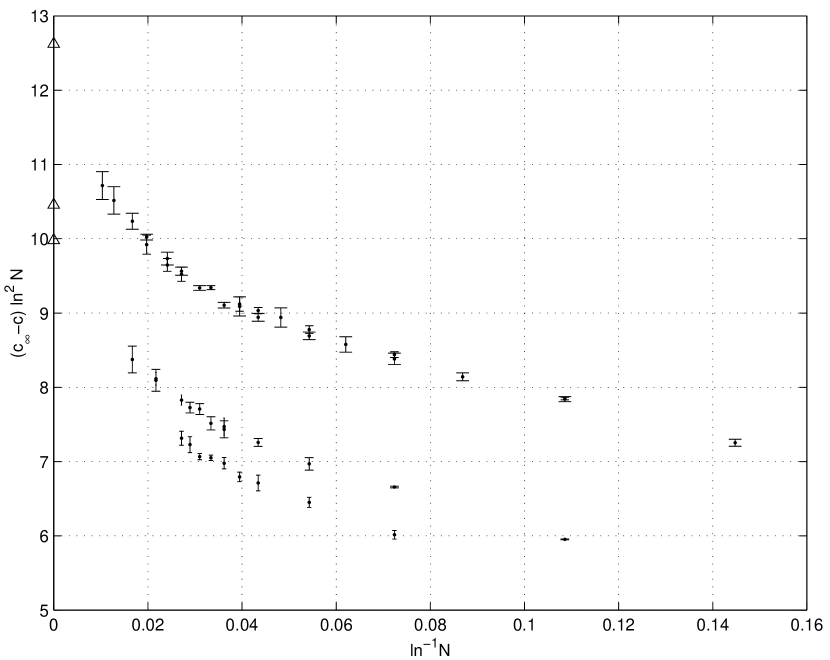
FIG. 6.: Front speed for the Langevin equation with parameters $\Delta t=0.01$ and $h=1$, $h=1/2$, $h=1/3$ correspondingly from top to bottom. Triangles on the $y$-axis are the corresponding asymptotic values for the deterministic cutoff.

REFERENCES

- [1] A. I. Kolmogorov, I. Petrovsky and N. Piscounov, Moscow Univ. Bull. Math. 1, 1 (1937).
- [2] I. Golding, Y. Kozlovsky and I. Cohen and E. Ben-Jacob, em Physica A, in press (1998) and references therein.
- [3] For a review, see D. A. Kessler, J. Koplik and H. Levine, Adv. Phys. 37, 255 (1988).
- [4] R. A. Fisher, Annual Eugenics, 7, 255 (1937).
- [5] E. Ben-Jacob, H. Brand, G. Dee, L. Kramer and J.S. Langer, Physica D, 14, 348 (1985); W. Van Saarloos, Phys. Rev A 39, 6367 (1989); G. C. Paquette, L.-Y. Chen, N. Goldenfeld and Y. Oono, Phys. Rev. Lett. 72, 76 (1994).
- [6] D. G. Aronson and H. F. Weinberger in Lecture Notes in Mathematics; Partial Differential Equations and Related Topics , A. Dold and B. Eckmann eds., Springer-Verlag (Berlin, 1975).
- [7] N. G. van Kampen, Stochastic Processes in Physics and Chemistry (North-Holland, Amsterdam, 1981)
- [8] E. Brener, H. Levine and Y. Tu, Phys. Rev. Lett., 66, 1978 (1990).
- [9] T.B. Kepler and A.S.Perelson, Proc. Natl. Acad. Sci. USA, 92(18), 8219 (1995).
- [10] L. Tsimring, H. Levine, and D. A. Kessler, Phys. Rev. Lett.76, 4440 (1996).
- [11] E. Brunet, B. Derrida, Phys. Rev. E 56, 2597 (1997).
- [12] D. A. Kessler, Z. Ner, L. M. Sander, Phys. Rev. E 58, 107 (1998).
- [13] D. A. Kessler and H. Levine, Nature 394, 556 (1998).
- [14] M. Doi, J. Phys. A 9, 1479 (1976).
- [15] L. Peliti, J. de Physique 46, 1469 (1985).
- [16] J. L. Cardy, U. C. Täuber, J. Stat. Phys. 90, 1, (1998) and references therein.
- [17] M. Cafaloni, E. Onofri, Nuclear Phys. B 151, 118 (1979).
- [18] G. W. Gardiner, Handbook of Stochastic Methods (Springer, Berlin, 1985).
- [19] R. Dickman, Phys. Rev. E 50, 4404 (1994).
- [20] W. Feller,Ann. Math. 54, 173 (1951); H.-J. Buttler and J. Waldvogel, Mathematical Finance 6, 53 (1996); J. Pitman and M. Yor, Z. Wahrschein. verw. Gebiete 59, 452 (1982).
- [21] A. Lemarchand, A. Lesne, and M. Mareschal, Phys. Rev. E 51, 4457 (1995).
- [22] M. Bramson, Mem. Am. Math. Soc. 44, No. 285 (1983).
- [23] J. Riordan, C. R. Doering and D. Ben-avraham, Phys. Rev. Lett. 75, 656 (1995).