Life and Death near a Windy Oasis

Abstract

We propose a simple experiment to study delocalization and extinction in inhomogeneous biological systems. The nonlinear steady state for, say, a bacteria colony living on and near a patch of nutrient or favorable illumination (“oasis”) in the presence of a drift term (“wind”) is computed. The bacteria, described by a simple generalization of the Fisher equation, diffuse, divide $A\rightarrow A+A$, die $A\rightarrow 0$, and annihilate $A+A\rightarrow 0$. At high wind velocities all bacteria are blown into an unfavorable region (“desert”), and the colony dies out. At low velocity a steady state concentration survives near the oasis. In between these two regimes there is a critical velocity at which bacteria first survive. If the “desert” supports a small nonzero population, this extinction transition is replaced by a delocalization transition with increasing velocity. Predictions for the behavior as a function of wind velocity are made for one and two dimensions.

PACS numbers: 05.70.Ln,87.22.As,05.40.+j

I Introduction and Results

Bacterial growth in a petri dish, the basic experiment of microbiology, is a familiar but interesting phenomenon. Depending on the nutrient and agar concentration, a variety of intriguing growth patterns have been observed[1, 2, 3, 4]. Some regimes can be modeled by diffusion limited aggregation, others by Eden models, and still others exhibit ring structures or a two-dimensional modulation in the bacterial density. At high nutrient concentration and low agar density, there is a large regime of simple growth of a circular patch (after point innoculation), described by a Fisher equation[5], and studied experimentally in Ref.[1].

Of course, most bacteria do not live in petri dishes, but rather in inhomogeneous environments characterized by, e.g., spatially varying growth rates and/or diffusion constants. Often, as in the soil after a rain storm (or in a sewage treatment plant), bacterial diffusion and growth are accompanied by convective drift in an aqueous medium through the disorder. By creating artificially modulated growth environments in petri dishes, one can begin to study how bacteria (and other species populations) grow in circumstances more typical of the real world. More generally, the challenges posed by combining inhomogeneous biological processes with various types of fluid flows[6] seem likely to attract considerable interest in the future. The easiest problem to study in the context of bacteria is to determine how fixed spatial inhomogeneities and convective flow affect the simple regime of Fisher equation growth mentioned above.

A delocalization transition in inhomogeneous biological systems has recently been proposed, focusing on a single species continuous growth model, in which the population disperses via diffusion and convection[7]: the Fisher equation[5] for the population number density $c({\mathbf{x}},t)$, generalized to account for convection and an inhomogeneous growth rate, reads [7, 8]

$$\partial c({\mathbf{x}},t)/\partial t = D\nabla^{2}c({\mathbf{x}},t)-{\mathbf{v}}\cdot\nabla c({\mathbf{x}},t)$$ (2)

$$+U({\mathbf{x}})c({\mathbf{x}},t)-bc^{2}({\mathbf{x}},t)\,,$$

where $D$ is the diffusion constant of the system, ${\mathbf{v}}$ is the spatially homogeneous convection (“wind”) velocity, and $b$ is a phenomenological parameter responsible for the limiting of the concentration $c({\mathbf{x}},t)$ to some maximum saturation value (by competition processes of the kind $A+A\rightarrow 0$[8]). The growth rate $U({\mathbf{x}})$ is a random function which describes a spatially random nutrient concentration, or, for photosynthetic bacteria, an inhomogeneous illumination pattern [7]. If $U({\mathbf{x}})$ is constant over the entire sample, then the convection term $-{\bf v}\cdot\nabla c({\bf x},t)$ has no effect on the growth of the bacteria. Only the introduction of a spatial dependence for the growth rate $U({\mathbf{x}})$ makes the convection term interesting. In the following we consider the simple case of a “square-well potential” shape for $U({\mathbf{x}})$, imposing a positive growth rate $a$ on an illuminated patch (“oasis”), and a negative growth rate $-\epsilon a$ outside (“desert”) [9]:

$$U({\mathbf{x}})=\cases{a\,,&for $|{\mathbf{x}}|<{W\over 2}\,,$\cr\ &\cr-\epsilon a\,,&for $|{\mathbf{x}}|\geq{W\over 2}\,,$\cr}$$ (3)

where $W$ is the diameter of the oasis. Experimentally this could be realized using a very simple setup, which both illustrates the basic ideas of localization and delocalization, and leads to interesting further questions. A one dimensional example is shown in figure 1, where a solution with photosynthetic bacteria in a thin circular pipe, or annular petri dish, is illuminated by a fixed uniform light source through a mask, leading to a “square well” intensity distribution. The mask is moved at a small, constant velocity around the sample to simulate convective flow. (Moving the mask is equivalent to introducing convective flow in the system, up to a change of reference frame[10].) The bacteria are assumed to divide in the brightly illuminated area (“oasis”) at a certain rate, but division ceases or proceeds at a greatly reduced rate in the darker region (“desert”) outside. As a result, the growth rate in this continuum population dynamics model is positive in the oasis and small (positive or negative) in the surrounding desert region. Using this simple nonlinear growth model, we discuss predictions for the total number of bacteria expected to survive in the steady state, the shape of their distribution in space and other quantities, as a function of the “convection velocity” of the light source.

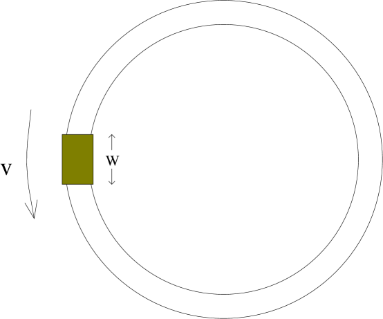
FIG. 1.: Experimental setup: a solution with photosynthetic bacteria in a circular pipe or a thin annular track in a petri dish, is illuminated only in a small area, while the rest of the sample is either kept dark or illuminated with reduced intensity. The light source is moved slowly around the sample to model convective flow. The bacteria are assumed to divide in the illuminated area (“oasis”) at a certain growth rate $a>0$, and die (or grow modestly) in the remaining area (“desert”) with growth rate $-\epsilon a$.

It is interesting to consider the class of biological situations discussed in this paper in the context of the ”critical size problem” in population dynamics [11]. In the critical size problem one asks for the minimal size of habitat for the survival of a population undergoing logistic growth and diffusion, where the region is surrounded by a totally hostile environment, i.e., no drift and an infinite death rate outside the oasis. We show here that the linearized version of the critical size problem is closely related to a well known problem in quantum mechanics, and present a generalization of this problem to include other types of surrounding environments, as well as the effect of drift. The linearized version of equation (2) around $c({\mathbf{x}},t)=0$ reads

$$\partial c({\mathbf{x}},t)/\partial t={\cal L}c({\mathbf{x}},t)\,,$$ (4)

with the linearized growth operator

$${\cal L}=D\nabla^{2}-{\mathbf{v}}\cdot\nabla+U({\mathbf{x}})\,.$$ (5)

(We discuss later the validity of this linear approximation and compare the results with lattice simulations of the full nonlinear problem.) For nonzero convection velocity $v$, ${\cal L}$ is non-Hermitian, but it can still be diagonalized by a complete set of right and left eigenvectors, $\{\phi^{R}_{n}({\mathbf{x}})\}$ and $\{\phi^{L}_{n}({\mathbf{x}})\}$, with eigenvalues $\Gamma_{n}$ [12, 7], and orthogonality condition

$$\int d^{d}x\phi^{L}_{m}({\mathbf{x}})\phi^{R}_{n}({\mathbf{x}})=\delta_{m,n}\,,$$ (6)

($d$ is the dimension of the substrate, we focus here on $d=1$ or $d=2$). The time evolution of $c({\mathbf{x}},t)$ is then given by

$$c({\mathbf{x}},t)=\sum_{n}c_{n}\phi^{R}_{n}({\mathbf{x}})\exp(\Gamma_{n}t)\,,$$ (7)

where the initial conditions and left eigenfunctions determine the coefficients $\{c_{n}\}$,

$$c_{n}=\int d^{d}x\phi^{L}_{n}({\mathbf{x}})c({\mathbf{x}},t=0)\,.$$ (8)

Figure 2 shows the complex eigenvalue spectrum with the potential (3) for four different values of the convection velocity $v$, for a one dimensional lattice approximation to (5) (see Appendix A) with periodic boundary conditions. The derivation of these results is discussed in section II below. At zero velocity $\cal{L}$ is Hermitian and all eigenvalues $\Gamma_{n}$ are real. There are bound states (discrete spectrum) and extended or delocalized states (continuous spectrum). At finite velocities, all except one of the delocalized states acquire a complex eigenvalue. States with positive real part of the eigenvalue ($Re{\Gamma_{n}}>0$) grow exponentially with time, states with negative real part ($Re{\Gamma_{n}}<0$) decrease exponentially with time (see Eq. (7)). In a large one dimensional system the “mobility edge”[13], which we define to be the eigenvalue of the fastest growing delocalized state, (i.e. the rightmost eigenvalue in the complex parabolas of figure 2), is located at the overall average growth rate

$$\Gamma^{*}=\langle U\rangle\equiv\int_{0}^{L}dxU(x)/L\simeq-\epsilon a\,,$$ (9)

(up to corrections of order $O(1/L)$ where the system size $L$ is the mean circumference of the annulus in figure 1). In figure 2, the eigenvalues of the localized states compose the discrete, real spectrum to the right of the mobility edge. With increasing velocity these localized eigenvalues move to the left by an amount proportional to $v^{2}/4D$, and successively enter the continuous delocalized spectrum through the mobility edge, which remains fixed. The parabola broadens in the vertical direction – the imaginary parts of the eigenvalues of the delocalized states grow by an amount proportional to $v$. A given localized right eigenfunction $\phi_{n}^{R}$ undergoes a “delocalization transition” when the velocity reaches a corresponding critical delocalization velocity $v=v^{*}_{n}$, at which its eigenvalue $\Gamma_{n}$ has been shifted so far to the left that it just touches $\Gamma^{*}$. At higher velocities it joins the parabola of eigenvalues describing a continuum of delocalized states. The ease with which such a delocalization transition can be observed experimentally depends on whether there are growing delocalized eigenstates in the system, i.e. whether the mobility edge has a positive real value or not.

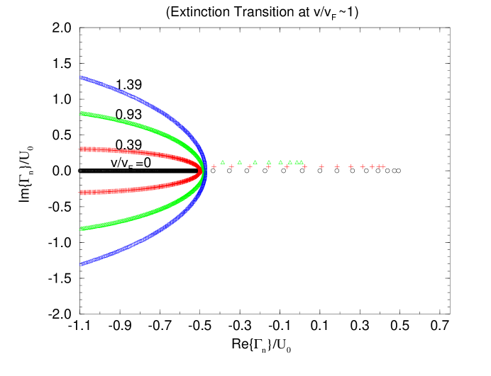
FIG. 2.: Complex nonhermitian eigenvalue spectra (normalized by the difference of the growth rates inside and outside the oasis $U_{0}=a+\epsilon a=1$) at velocities above and below the extinction transition. The spectra are extracted from numerical simulations of the lattice model described in Appendix B, for a system of 1000 sites, oasis width $W=20$ sites, $D=0.3$, with growth rate $U=-0.5$ in the desert and $U=+0.5$ in the oasis, so that the average growth rate is is $-0.48$ (which is equal to the mobility edge $\Gamma^{*}$ up to finite size effects). The chosen velocity parameters (in units of the Fisher wave velocity in the oasis $v_{F}=2\sqrt{aD}$ [5]) are $v/v_{F}\sim 0$ (circles), $v/v_{F}\sim 0.39$ (plus), $v/v_{F}\sim 0.93$ (triangles), and $v/v_{F}\sim 1.39$ (squares). The point spectra are slightly offset in the $y$-direction so as to be able to distinguish the eigenvalues of the localized states for different velocities. As described in the introduction, the mobility edge remains roughly fixed, and the parabola of the delocalized eigenvalues opens up as $v/v_{F}$ is increased. The real, localized eigenvalues move to the left for higher velocities. At $v/v_{F}\geq 1.39$ all states are delocalized. (This figure actually only shows the part of the spectrum which corresponds to the continuum problem. The lattice calculation also yields a left part of the spectrum – not shown here – which is an artifact of the discrete lattice.)

In a large “deadly” desert ($\langle U\rangle\simeq-\epsilon a<0$) all delocalized states die out, because the mobility edge lies to the left of the origin, as in figure 2. The growth rate of each localized eigenstate $\phi^{R}_{n}$ then becomes negative at a corresponding “extinction” velocity $v_{nc}$ which is smaller than the corresponding delocalization velocity $v^{*}_{n}$. Thus, as convection is increased, the population dies out before it can delocalize. Later in this paper, we make specific predictions for the behavior of populations near the extinction transition, which occurs for $v=v_{0c}>v_{nc}$ for all $n>0$, when the eigenvalue of the localized “ground state” (fastest growing eigenfunction of $\cal{L}$) passes through the origin.

If the average growth rate $\langle U\rangle$ is positive (i.e for a small enough desert or a small positive growth rate in an infinite desert), the mobility edge lies to the right of the origin and the delocalization transition can indeed be observed at $v=v_{0}^{*}$ where the “ground state” becomes delocalized. One expects to see universal behavior near this delocalization transition, since there is a diverging correlation length in the system, which renders microscopic details irrelevant for certain quantities. We report predictions (see also [14]), for quantities such as the dependence of the localization length on the drift velocity as it approaches the delocalization velocity, and the shape of the concentration profile near the transition.

A special (universal) behavior is expected for the spatially average growth rate $\langle U\rangle=0$. In this case the delocalization and extinction velocities coincide. Figure 3 summarizes the different scenarios in a sketch of the phase diagram for large systems with fixed well depth $U_{0}\equiv(a+\epsilon a)$, tuning the drift velocity, and the average growth rate $\langle U\rangle=-\epsilon a$. Also shown in figure 3 is a horizontal transition line at $\langle U\rangle=0$ separating a small velocity region ($\epsilon<0$) where localized modes dominate the steady state bacterial population, from one ($\epsilon>0$) containing a mixture of localized and extended states. The experimental signature of this interesting transition, (which could be accessed by increasing the light intensity for photosynthetic bacteria at fixed convection velocity) will be discussed in a future publication [14]. It is of course also possible to drive a population extinct at zero velocity simply by lowering the average growth rate. This special transition at $\langle U\rangle=-U_{c}$ is indicated at the bottom of figure 3.

FIG. 3.: Schematic phase diagram in one dimension for infinite system size, as a function of average growth rate $\langle U\rangle$ and convection velocity $v$. For a deep well ($U_{0}\equiv a+\epsilon a\gg D/W^{2}$) the extinction transition out of the localized phase occurs when $v=0$ for $\langle U\rangle=-U_{c}$, where $U_{c}\simeq U_{0}$. The diagram shows that if the growth rate is negative outside and inside the oasis (i.e. $\langle U\rangle<-U_{c}$), then the only possible state is extinction at any velocity. If there is positive growth inside the oasis, but negative outside, a localized population can survive in the oasis, but only for small enough wind velocities $v$. Extended states are present for a small positive growth rate in the desert ($\langle U\rangle>0$). In this case localized and delocalized states coexist for small velocities (“mixed phase”), while at large velocities all eigenstates are extended, as shown in figure 6. The ground state becomes delocalized at the critical velocity $v_{c}$ which marks the phase boundary between the mixed and the extended phase.

In section II we give details of the analysis of the one dimensional linearized problem for infinite and finite systems with periodic boundary conditions. In section III some effects of the nonlinear term are discussed, especially for experiments near the extinction transition, and in section IV the two dimensional case is discussed. The appendices contain some details on the analytic computation of finite size effects (Appendix A), a brief discussion of a lattice model [7] corresponding to the analytic continuum theory (Apppendix B), and a discussion of dimensionless quantities measurable in experiments (Appendix C).

II Linearized Growth in one Dimension

If the left and right eigenfunctions $\phi^{R,L}_{n}({\mathbf{x}})$ are localized (i.e. if the convection velocity is small enough, so that $\phi^{R,L}_{n}({\mathbf{x}})$ decays exponentially with the distance from the oasis), one may eliminate the convective term in Eq. (5) via the transformation

$$\phi^{R,L}_{n}({\mathbf{x}})=\exp(\pm{\mathbf{v}}\cdot{\mathbf{x}}/2D)\psi_{n}({\mathbf{x}})$$ (10)

($+$ refers to the right eigenvectors and $-$ to the left eigenvectors). The eigenvalue equation associated with the linearized growth operator (4) becomes Hermitian [15]

$$\Gamma_{n}\psi_{n}({\mathbf{x}})=D\nabla^{2}\psi_{n}({\mathbf{x}})+U({\mathbf{x}})\psi_{n}({\mathbf{x}})-(v^{2}/4D)\psi_{n}({\mathbf{x}})\,,$$ (11)

and is equivalent to the familiar square well potential problem much studied in quantum mechanics. With the identifications $a+\epsilon a\equiv U_{0}/{\hbar}$, where $U_{0}$ is a quantum well depth, and ${\hbar}$ is Planck’s constant, $\Gamma_{n}+\epsilon a+v^{2}/4D\equiv|E|/\hbar$, where $E$ is a quantum energy level, and $D\equiv\hbar/2m$, where $m$ is a mass in the equivalent quantum problem, we can use well known quantum mechanical results[16, 17]. The left and right eigenfunctions at finite velocity are then related to the eigenstates of the Hermitian problem (11) via the transformation (10), while the eigenvalues undergo a rigid shift

$$\Gamma_{n}(v)=\Gamma_{n}(v=0)-{v^{2}\over 4D}.$$ (12)

A An Oasis in an Infinite Desert: Localized Populations and the Extinction Transition

In an infinite one dimensional system, localized solutions for $\phi^{R,L}_{n}(x)$ are given by Eq. (10) with [18]

$$\psi_{n}(x)=\cases{A_{1,n}\exp(\kappa_{n}x)\,,&for $x<-{W\over 2}\,,$\cr\ &\cr B_{1,n}\exp(ik_{n}x)+B_{2,n}\exp(-ik_{n}x)\,,&for $-{W\over 2}<x<{W\over 2}\,,$\cr\ &\cr A_{2,n}\exp(-\kappa_{n}x)\,,&for $x>{W\over 2}\,,$\cr}$$ (13)

where $A_{1,n},A_{2,n},B_{1,n},$ and $B_{2,n}$ are constant coefficients, and

$$\kappa_{n}=\sqrt{(\Gamma_{n}(v=0)+\epsilon a)/D}\,,$$ (14)

and

$$k_{n}=\sqrt{(a-\Gamma_{n}(v=0))/D}\,,$$ (15)

as can be seen by substituting the above Ansatz for $\psi(x)$ into Eq. (11). Eq. (14) implies

$$\Gamma_{n}(v=0)=D\kappa_{n}^{2}-\epsilon a\,.$$ (16)

To compute $\Gamma_{n}(v=0)$ one matches both $\psi_{n}(x)$ and $\partial\psi_{n}(x)/\partial x$ at $x=\pm W/2$, which determines the coefficients $A_{i,n},B_{i,n}$, $i=1,2$, up to an overall multiplicative factor, as well as the eigenvalues $\{\Gamma_{n}(v=0)\}$. When solving the Hermitian problem one may use the fact that all the eigenfunctions admit a well defined parity, i.e., they are odd or even under the transformation $x\rightarrow-x$. Even integers $n$ correspond to bound eigenstates with even parity, where $\psi_{n}(x)$, is symmetric under $x\rightarrow-x$. In such a case one obtains the eigenvalue equation for the quantity

$$\zeta_{n}(\Gamma_{n})\equiv k_{n}W/2=W/2\sqrt{(a-\Gamma_{n}(v=0))/D}\,,$$ (17)

namely,

$$\cot(\zeta_{n})=\zeta_{n}{\bar{x}}/\sqrt{1-(\zeta_{n}{\bar{x}})^{2}}\,,$$ (18)

(which is equivalent to $\cot(k_{n}W/2)=k_{n}/\kappa_{n}$), with

$$\bar{x}=2\sqrt{D/(a+\epsilon a)}/W=2/(\sqrt{k_{n}^{2}+\kappa_{n}^{2}}W)\,.$$ (19)

The dimensionless parameter ${\bar{x}}$ measures the ratio of kinetic to potential energy in the equivalent quantum problem. For bound eigenstates with odd parity $\psi(x)$, ($\psi(x)$ antisymmetric under $x\rightarrow-x$, denoted by odd $n$ ) one obtains

$$\cot(\zeta_{n})=-\sqrt{1-(\zeta_{n}{\bar{x}})^{2}}/(\zeta_{n}{\bar{x}})\,.$$ (20)

The highest eigenvalue (with its nodeless, positive eigenfunction $\psi_{0}(x)$), corresponds to the largest growth rate $Re\{\Gamma_{0}\}$, and is therefore expected to dominate the system in most cases at long times, as seen from Eq. (7). Its eigenvalue condition (18) for $n=0$ leads to [16]

$$\Gamma_{0}(v=0)+\epsilon a=(a+\epsilon a)f(\bar{x})\,,$$ (21)

where $f({\bar{x}})$ is a monotonically decreasing function such that $f(\bar{x})\simeq 1-\pi^{2}\bar{x}^{2}/4$ for $\bar{x}\ll 1$, and $f(\bar{x})\simeq 1/\bar{x}^{2}$ for $\bar{x}\gg 1$. Upon inserting Eq. (21) into the expressions for $\kappa_{n}$ and $k_{n}$ one obtains

$$\kappa_{0}=\sqrt{(a+\epsilon a)f(\bar{x})/D}$$ (22)

and

$$k_{0}=\sqrt{((a+\epsilon a)(1-f(\bar{x})))/D}\,.$$ (23)

When $\bar{x}\ll 1$, the “potential well” is very deep, and one finds the usual particle in a box result for $\Gamma_{0}(v)$, with correction term proportional to $v^{2}$ arising from the change of variables (10) and (12), namely

$$\Gamma_{0}(v)\simeq(v_{c}^{2}-v^{2})/(4D)=a-D\pi^{2}/W^{2}-v^{2}/4D\,,$$ (24)

with

$$v_{c}=2D\sqrt{(a/D-\pi^{2}/W^{2})}\,,$$ (25)

$$\kappa_{0}=\sqrt{(a+\epsilon a)/D-\pi^{2}/W^{2}}\,$$ (26)

and

$$k_{0}=\pi/W\,.$$ (27)

For $\bar{x}\gg 1$ one finds

$$\Gamma_{0}(v)\simeq(v_{c}^{2}-v^{2})/(4D)=(a+\epsilon a)^{2}(W/2)^{2}/D-\epsilon a-D(v/2D)^{2}$$ (28)

with

$$v_{c}=2D\sqrt{((a+\epsilon a)W/2)^{2}/D^{2}-\epsilon a/D}\,,$$ (29)

$$\kappa_{0}=\sqrt{(a+\epsilon a)^{2}(W/2)^{2}/D^{2}}$$ (30)

and

$$k_{0}=\sqrt{(a+\epsilon a)(1-1/\bar{x}^{2})/D}\,.$$ (31)

If we take as an effective diffusion constant for motile bacteria $D=6\cdot 10^{-6}{\text{c}m}^{2}/{\text{s}ec}$, and a growth rate $a=10^{-3}$ /sec in the oasis and a much smaller growth rate outside ($0<|\epsilon|<<1$), we get for a $W=2{\text{c}m}$ diameter oasis, $\bar{x}=0.077\ll 1$, and an “extinction velocity” $v_{c}\simeq 1.5\mu/{\text{s}ec}$, which is comparable to the Fisher wave velocity [5] in the oasis, $v_{F}=2\sqrt{aD}=1.5\mu/{\text{s}ec}$.

B Finite Size Effects and the Delocalization Transition

An experimental finite system with periodic boundary conditions is depicted in figure 1. The eigenvalue equation for $\kappa_{n}(\Gamma_{n})$ and $k_{n}(\Gamma_{n})$ of the corresponding linearized problem of an oasis of width $W$ in a finite desert of extent $L>W$ (with $L$ being the mean circumference of the circular region in figure 1), is obtained using the Ansatz in Eq. (10) with

$$\psi_{n}(x)=\cases{(A_{1,n}\exp(\kappa_{n}x)+A_{2,n}\exp(-\kappa_{n}x))\,,&for $-{L\over 2}<x<-{W\over 2}\,,$\cr\ &\cr(B_{1,n}\exp(ik_{n}x)+B_{2,n}\exp(-ik_{n}x))\,,&for $-{W\over 2}<x<{W\over 2}\,,$\cr\ &\cr(C_{1,n}\exp(\kappa_{n}x)+C_{2,n}\exp(-\kappa_{n}x))\,,&for ${W\over 2}<x<{L\over 2}\,,$\cr}$$ (32)

and matching $\phi^{R,L}_{n}(x)$ and $d\phi^{R,L}_{n}(x)/dx$ at the edges of the well and at the edges of the sample (imposing periodic boundary conditions). One finds the eigenvalue equation[12] (see also [19])

$$2 k_{n}\kappa_{n}(cosh(Lv/(2D))-cos(k_{n}W)cosh(\kappa_{n}(L-W)))$$ (33)

$$+ (k^{2}_{n}-\kappa^{2}_{n})sin(k_{n}W)sinh(\kappa_{n}(L-W))=0\,.$$ (34)

For $v/(2D)<Re\{\kappa_{n}\}$, and large $L$, equation (33) yields

$$\exp(L(v/(2D)-\kappa_{n}))=$$ (35)

$$\cos(k_{n}W)-k_{n}/(2\kappa_{n})\cdot(1-(\kappa_{n}/k_{n})^{2})\sin(k_{n}W)\,.$$ (36)

The left hand side vanishes in the limit $L\rightarrow\infty$, and the equation reduces to the bound state equations of a single square well (Eq. (18) for even parity solutions and Eq. (20) for odd solutions). For finite $L$, and $v/2D<Re\{\kappa_{n}\}$, the deviation of the “localized” solutions $\kappa_{n}$ and $k_{n}$ from their $v=0$ values for small $v$ is exponentially small in L [12]. These “localized” or “bound state” solutions, are characterized by an exponential decay of the bacterial density in the desert with a correlation length

$$\xi_{n}\sim(Re\{\kappa_{n}\}-v/(2D))^{-1}$$ (37)

and $\Gamma_{n}(v)$ strictly real. However, “delocalized” or “scattering” solutions also exist, with $\Gamma_{n}(v)$ complex, and nontrivial dependence of $\kappa_{n}$ and $k_{n}$ on $v$, even in the limit of large $L$. As the velocity is increased, the $n$th localized eigenstate becomes delocalized ($\xi_{n}\rightarrow\infty$) at the critical delocalization velocity $v_{n}^{*}$ given in an infinite system by

$$v_{n}^{*}=2DRe\{\kappa_{n}\}\,.$$ (38)

This implies

$$\xi_{n}\sim 1/(v_{n}^{*}-v)^{\nu}$$ (39)

with the (universal) critical exponent $\nu=1$. We saw that with increasing velocity, the growth rate $Re\{\Gamma_{n}(v)\}$ for a given eigenstate decreases. It becomes negative above the corresponding extinction velocity $v_{nc}$. We therefore expect that the delocalization transition for the “ground state” (which tends to dominate the long time behavior) can be observed only if $v_{0}^{*}\leq v_{0c}$. In the following we discuss the three desert scenarios, $\epsilon>0$, $\epsilon<0$, and $\epsilon=0$.

(1) For $\epsilon>0$ (a “deadly” desert), of big enough size $L$, one finds that all delocalized states die out exponentially with time ($v_{nc}<v_{n}^{*}$). The population is localized around the oasis at small $v$ and extinct at high $v$. Figure 2 is a plot of the eigenvalues $\Gamma(v)$ in the complex plane for this case, as derived for the lattice model discussed in Appendix B. The lower part of figure 4 shows a series of profiles of the ground state eigenfunction close to the extinction transition. In small enough systems, such that the total effective growth rate $\int_{0}^{L}U(x)dx$ is positive, delocalized states can actually have a positive growth rate even for $\epsilon>0$. (See also Eq. (A4) in Appendix A, with $\delta\kappa\sim O(1/L)$, and ${\bar{\kappa}}\sim O(1/L)$ .) In this case, the system is small enough so that the bacteria can traverse the desert quickly, and on average won’t die before reenterring the oasis in a circular pipe.

(2) If $\epsilon<0$, delocalized states should be observable even for very large systems, because the “desert” can support modest growth, although at a much smaller rate than in the oasis if $|\epsilon|\ll 1$. Growing delocalized eigenstates are present, even for $v=0$, and the population is a superposition of fast growing localized states and more slowly growing delocalized ones. As a drift velocity $v$ increases, the n’th localized eigenstate delocalizes at $v=v^{*}_{n}$ with a positive growth rate $Re{\Gamma_{n}(v^{*}_{n})}$ (i.e. $v^{*}_{n}<v_{nc}$). This case allows for an experimental observation of the delocalization transition: as the velocity is increased, more and more eigenstates delocalize. The eigenvalue spectrum for two different values of $v$ is shown in figure 5 (a) and (b). We can see that the spectrum at the delocalization transition is slightly different depending on whether an “even” eigenfunction or an “odd” eigenfunction is about to delocalize next (“even” and “odd” are to be understood in the sense explained in section II A). If an odd eigenfunction is about to delocalize next, there exists a delocalized state which has a purely real growth rate (at the tip of the parabola in the spectrum of figure 5(b)), while no such state exists when an even eigenfunction is about to delocalize, as in figure 5(a). The essential characteristics of the spectrum are derived in Appendix A.

For experiments, we focus on the delocalization of the ground state, since it is the fastest growing eigenstate, which dominates the system near the oasis. The ground state delocalizes at the highest delocalization velocity $v=v^{*}_{0}$, i.e. for $v>v^{*}_{0}$ all states are delocalized. The lower part of figure 6 shows a series of profiles of the ground state eigenfunction close to delocalization. One sees that at the delocalization velocity $v^{*}_{0}$, the correlation length $\xi_{0}$ reaches the system size. In an infinite system it diverges as in Eq. (39). Near the delocalization transition, we expect certain quantities to become independent of microscopic details of the system. These universal quantities will only depend on general properties, such as symmetries, dimensions etc.. Simple models that only share these general properties with the experimental system will be sufficient for precise predictions for these quantities near the transition. An example of such a quantity is the critical exponent $\nu$ in Eq. (39). Details for the square well system and more general random systems will be presented in a future paper[14].

(3) For $\epsilon=0$, the growth rate of the bacteria exactly balances the death rate in the desert, they only diffuse. In this case the delocalization velocity and the extinction velocities coincide: $v^{*}_{n}=v_{nc}$ in an infinite system. There is again a diverging correlation length leading to universal critical behavior near the delocalization transition [14]. In a finite system the average growth rate $\int_{0}^{L}dxU(x)/L$ is positive. In small systems, one therefore expects to see delocalized states with a positive growth rate in experiments for this case as well.

These results for one dimension in the limit $L\rightarrow\infty$ are summarized in figure 3 which shows a schematic phase diagram for fixed well depth $U_{0}\equiv(a+\epsilon a)$, as a function of the convection velocity and the average growth rate $\langle U\rangle\equiv\int_{0}^{L}dxU(x)/L$, in the limit $L\rightarrow\infty$.

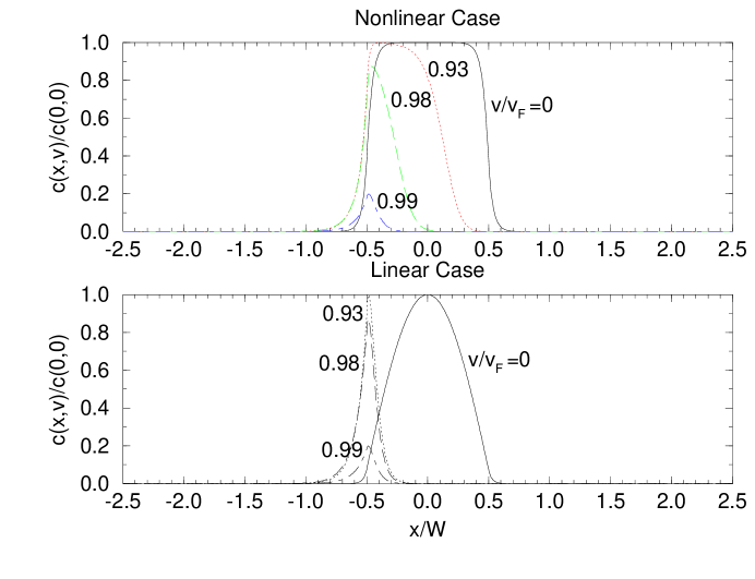
FIG. 4.: A series of steady state population profiles for a system with negative average growth rate, at different drift velocities, for the linear and the nonlinear case. The $x$ coordinate is normalized by the width $W$ of the oasis. In the nonlinear case the populations $c(x,v)$ are divided by the population at zero velocity in the middle of the oasis $c(0,0)$. In the “linear” case, we simply assume the validity of Eq. (47) and rescale the curves such that their maximum values match those of the nonlinear case. The profiles were extracted from a lattice model with 1000 sites, an oasis of width $W=200$ sites, with growth rate $U=0.5$ inside the oasis and $U=-0.5$ outside, and diffusion constant $D=30$. The velocity parameters are taken to be $v/v_{F}=0$ (solid line), $v/v_{F}=0.93$ (dotted), $v/v_{F}=0.98$ (dashed), and $v/v_{F}=0.99$ (dash-dotted). Close to the extinction transition, where the population is small, the agreement between the nonlinear and the linear solution becomes quite good. The oasis occupies the region $|x/W|<0.5$ in the figures.

FIG. 5.: Sketches of complex nonhermitian eigenvalue spectra at two different velocities: (a) velocity $v_{a}$ with $v_{7}^{*}<v_{a}<v_{6}^{*}$, where $n=6$ denotes an even eigenstate, i.e. all eigenstates with $n>6$ are delocalized and those with $n\leq 6$ are localized; and (b) at a higher velocity $v_{b}>v_{a}$ with $v_{6}^{*}<v_{b}<v_{5}^{*}$ where $n=5$ denotes an odd eigenstate. Upon increasing the velocity from $v_{a}$ to $v_{b}$ the $n=6$ eigenstate becomes delocalized at $v=v^{*}_{6}$.

FIG. 6.: A series of steady state population profiles for a system with positive average growth rate, at different drift velocities, for the linear and the nonlinear case. The $x$ coordinate is normalized by the width $W$ of the oasis $(|x/W|\leq 0.5)$. In the nonlinear case the populations $c(x,v)$ are divided by $c(0,0)$, the population in the middle of the oasis, at zero velocity. Curves for the “linear” case, were computed as in figure 4. The profiles were extracted from a lattice model with 1000 sites, an oasis of width $200$ sites, with growth rate $U=0.1$ inside the oasis and $U=1.1$ outside, and large diffusion constant $D=300$. The velocity parameters $v/v_{F}$ are taken to be $v/v_{F}=0$ (solid line), $0.17$ (dotted), $0.33$ (dashed), $0.50$ (long-dashed), and $0.83$ (dash-dotted). In both cases the population becomes delocalized at high velocities with increasing velocity when the correlation length reaches the size of the system.

C Delta-Function Potential Well

Results for a delta-function-like oasis in one dimension, can be easily derived as a special case of the square well potential, by taking the limit $\epsilon\rightarrow 0$, $a\rightarrow\infty$ and $W\rightarrow 0$ with $aW={\text{c}onst}\equiv V_{0}$. In this case Eq. (33) simplifies to

$$\kappa(\cosh(Lv/(2D))-\cosh(\kappa L))+V_{0}\sinh(\kappa L)/D=0\,,$$ (40)

which is the same equation as obtained in [12]. With the identification $\kappa\equiv(-i)K$ the results derived there can be applied here: the delocalization picture is the same as in figure 5(a), except that there exists only one (even parity) bound state solution for $Re\{\kappa\}>v/(2D)$. Again two critical velocities $v_{c0}$ and $v^{*}_{0}$ emerge, in accordance to the above discussion for a square well potential.

III Effects of the Nonlinearity

We can also estimate the effects due to the nonlinear term in equation (2), which leads to a saturation of $c(x,t)$ for $\Gamma_{n}(v)>0$. The equation of motion becomes

$$\partial c(x,t)/\partial t={\cal L}c(x,t)-bc^{2}(x,t)\,,$$ (41)

with $\cal L$ given by Eq. (5). (The coefficient $b$ can be set to 1 by rescaling the density $c(x,t)$ by $b$, as in Appendix C.) The solution can be expressed in terms of the complete set of right eigenstates for the linear problem with new time dependent coefficients $c_{n}(t)$ with

$$c(x,t)=\sum_{n}c_{n}(t)\phi^{R}_{n}(x)$$ (42)

and

$$dc_{n}(t)/dt=\Gamma_{n}c_{n}(t)-\sum_{m,m^{\prime}}w_{n,mm^{\prime}}c_{m}(t)c_{m^{\prime}}(t)\,,$$ (43)

where the mode couplings are given by [7]

$$w_{n,mm^{\prime}}=b\int dx\phi_{n}^{L}(x)\phi_{m}^{R}(x)\phi_{m^{\prime}}^{R}(x)\,.$$ (44)

In general one expects that through the mode couplings the fastest growing eigenstate suppresses the growth rate of the other eigenstates, provided the corresponding couplings are large enough [7, 14]. In the mixed phase of figure 3 we expect that the fastest growing bound state suppresses the other bound states, and the fastest growing delocalized state suppresses the other delocalized states[14].

A Effects of the Nonlinearity at the Extinction Transition

For $\epsilon>0$ (and large enough systems so that $\int_{0}^{L}dxU(x)<0$), with velocity $v$ just below the extinction velocity $v_{0c}$, we expect that the growing ground state term $c_{0}(t)\phi^{R}_{0}(x)$ dominates the summation (42) for $c(x,t)$. In a first approximation we neglect all $c_{m}(t)$ with $m>0$ and find

$$dc_{0}(t)/dt=\Gamma_{0}c_{0}(t)-w_{0}c_{0}^{2}(t),$$ (45)

with $w_{0}\equiv w_{0,00}=b\int d^{d}x\phi^{L}_{0}(x)(\phi^{R}_{0}(x))^{2}>0$. At long times

$$c_{0}(t)=c_{0}(0){\frac{\exp(\Gamma_{0}t)}{1+c_{0}(0)(\exp(\Gamma_{0}t)-1)w_{0}/\Gamma_{0}}}$$ (46)

with asymptotic behavior $\lim_{t\rightarrow\infty}c_{0}(t)=\Gamma_{0}/w_{0}$. Thus, the steady state population profile should be given approximately by

$$c^{*}(x)=\Gamma_{0}\phi^{R}_{0}(x)/w_{0}\,,$$ (47)

where

$$c^{*}(x)={\text{l}im}_{t\rightarrow\infty}c(x,t)\,.$$ (48)

The total steady state bacterial population $N_{0}$ is

$$N_{0}=\int dxc^{*}(x)\,.$$ (49)

It follows that

$$N_{0}\simeq(\Gamma_{0}/w_{0})\int dx\phi^{R}_{0}(x)\,.$$ (50)

Since $\Gamma_{0}\sim(v-v_{c})(v+v_{c})$, and $\int dx\phi^{R}_{0}(x)\sim{\text{c}onst}+O(v-v_{c})$ as $v\rightarrow v_{c}$ from below, one finds that near the extinction transition

$$N_{0}\sim\cases{v_{c}-v\,,&for $v\rightarrow v_{c}^{-}\,,$\cr\ &\cr 0\,,&for $v>v_{c}\,,$\cr}$$ (51)

Figure 7 shows the total population $N_{0}$ as a function of the convection velocity $v$ for an oasis in a desert with negative growth rate, which is large enough so that the average growth rate is negative also. The data was obtained from a lattice model for the nonlinear problem (see Appendix A). The displayed convection velocities range from $v=0$ to velocities larger than the extinction velocity $v>v_{c}$. One can see that $N_{0}$ decreases linearly with $v-v_{c}$ for $v\rightarrow v_{c}^{-}$, as predicted in Eq. (51). Figure 4 shows a series of population profiles for increasing velocity, for the linear case (i.e. taking the ground state of the linear problem as a solution for the steady state), and for the nonlinear case. One can see that close to the extinction transition the ground state of the linearized growth is an excellent approximation, as is to be expected since there the bacterial density $c(x)$ becomes small, so that mode couplings other than $w_{0}$ induced by the nonlinear term $bc^{2}(x)$ become small relative to the linear terms.

FIG. 7.: Numerical results for the total number of bacteria $N_{0}(v)$ (normalized by the total number at zero velocity $N_{0}(0)$) as a function of $v/v_{F}$, where $v_{F}=2\sqrt{aD}$ is the Fisher wave velocity. The data were obtained using a 1 dimensional lattice model with 100 grid points (see Appendix B). The diffusion constant is $D=3.$, the width of the oasis is $W=20$, the growth rate is -0.9 outside the oasis and 0.1 inside. The coefficient of the nonlinear term in the equation of motion is $b\equiv 1$. The average growth rate is $-0.7<0$ for this system, so that $v_{0c}<v^{*}_{0}$, and the system goes through the extinction transition at $v/v_{F}\simeq 0.65$, above which $N_{0}(v)$ vanishes. The approximation $v_{c}\simeq v_{F}$ mentioned in the text does not work quite as well here as in other cases because the condition ${\bar{x}}\ll 1$ necessary for this approximation is violated weakly for the model parameters chosen here. (${\bar{x}}\simeq 0.35$).

B Limit $v\rightarrow 0$

In the linearized case, because Eq. (11) is even in $v$, we expect $N_{0}(t)=\int d^{d}xc({\mathbf{x}},t)\sim{\text{c}onst}-{\text{c}onst}^{\prime}\cdot v^{2}+O(v^{4})$ for small velocities. In the nonlinear case this symmetry is broken, because of the $v$ dependence of the coefficients $w_{nmm^{\prime}}$ in Eq. (44) which arises from the transformation (10). One then expects in the steady state $N_{0}\sim{\text{c}onst}-{\text{c}onst}^{\prime}\cdot|{\bf v}|+O(v^{2})$ for small velocities. The constants depend on $U(x)$ and other nonuniversal details.

C Effects of the Nonlinearity at the Delocalization Transition

Figure 6 shows the same information as figure 4 for the delocalization transition for an oasis in a background with positive growth rate. One can see that the linear approximation (i.e. taking the ground state of the linear problem as a solution for the steady state), becomes best for high velocities [14], when the drift term in the equation of motion becomes dominant compared to the nonlinear term. Furthermore the nonlinear solution at low velocities is in the “mixed phase”, i.e., it is a superposition of extended and localized eigenstates of the system. A decomposition of the $v=0$ nonlinear solution into the eigenstates of the system shows [14] that its leading contributions are from the localized ground state eigenfunction and the fastest growing delocalized eigenfunction. As the drift velocity is increased, the contribution of localized eigenstates clearly diminishes. Above the delocalization transition, the steady state is composed only of delocalized modes.

IV Two dimensions, infinite system size

Much of the above analysis can be adapted to two dimensions. We again use the transformation (10) and consider a circular oasis of diameter $W$ in Eq. (11). The analysis is straightforward, so we omit most of the details. Following reference[12], the qualitative behavior of non-Hermitian eigenvalue spectra for linearized growth in two dimensions should be as follows: As in one dimension, localized states associated with the potential well will lie in a point spectrum on the real axis. Extended states, however, will occupy a dense region in the complex plane with a parabolic boundary (see figure 8). With increasing $v$, the localized point spectrum will again migrate into the continuum.

FIG. 8.: Sketch of a complex nonhermitian eigenvalue spectrum in two dimensions with localized and delocalized eigenstates. The sketch uses a computation of the spectrum for a delta function potential in two dimensions [12], in which case there is only one bound state (to the right of the imaginary axis). We expect qualitatively the same result for the finite two dimensional well discussed in the text, except that multiple bound states with real eigenvalues will occur, just as in one dimension.

In the localized regime the spatial distribution of bacteria is in the linear approximation given by the convection-distorted ground state eigenfunction,

$$\phi^{R,L}_{0}({\mathbf{x}})=\cases{C_{1,0}\exp(\pm{\mathbf{v}\cdot x}/2D)J_{0}(k_{n}|{\mathbf{x}}|)\,,&for $|{\mathbf{x}}|<W/2\,,$\cr\ &\cr C_{2,0}\exp(\pm{\mathbf{v}\cdot x}/2D)K_{0}(\kappa_{n}|{\mathbf{x}}|)\,,&for $|{\mathbf{x}}|>W/2\,,$\cr}$$ (52)

where $J_{0}(x)$ and $K_{0}(x)$ are Bessel functions of order zero[20]. The constants $C_{1,0}$ and $C_{2,0}$ are chosen such that $\phi^{R,L}_{0}({\mathbf{x}})$ and its radial derivative are continuous at $|{\mathbf{x}}|=W/2$. The lowest energy eigenvalue is again given by eq. (21), but with different results for $f(\bar{x})$ [16]: for $\bar{x}\ll 1$ one finds $f(\bar{x})\simeq 1-a_{1}^{2}\bar{x}^{2}$ where $a_{1}\simeq 2.405$ is the first zero of $J_{0}(a)$; for $\bar{x}\gg 1$ one finds $f(\bar{x})\simeq\bar{x}^{2}\exp(-4\bar{x}^{2})$. The behavior of the ground state eigenvalue is thus

$$\Gamma_{0}\simeq a-4D(2.405)^{2}/W^{2}-Dv^{2}/(4D)$$ (53)

for $\bar{x}\ll 1$ and

$$\Gamma_{0}\simeq D(4/W^{2})\exp[-16D/(W^{2}(a+\epsilon a))]-D(v/2D)^{2}$$ (54)

for $\bar{x}\gg 1$. From these results one can compute $v_{0c}$ for the 2 dimensional case. As in one dimension, one again finds for $\epsilon>0$ (“deadly” oasis), and large enough systems, that $v_{c0}<v_{0}^{*}$, where $v_{0}^{*}/2D\simeq Re\{\kappa_{0}\}$, and $v_{0c}$ is the velocity above which the ground state growth rate $\Gamma_{0}$ becomes negative.

Figure 9 shows a contour plot for the spatial distribution of bacteria in the linearized case at convection velocity $v$ below $v_{0c}$ in 2 dimensions, obtained from equation (52). Although the full nonlinear two dimensional problem seems tractable numerically, we expect that close to the extinction transition the curves for the linearized case will approximate the shape of the steady state, because the ground state dominates sums like that in equation (42).

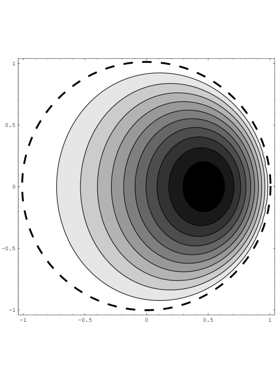
FIG. 9.: Contour plot of the distribution of bacteria in two dimensions as obtained for the linearized problem for convection velocity $v=0.2\mu/sec<v_{c}=1.5\mu/sec$ (directed to the right), with $D=6\cdot 10^{-6}{\text{c}m}^{2}/{\text{s}ec}$, and growth rate $a=10^{-3}$/sec in the oasis (of diameter $W=2{\text{c}m}$) and a much smaller growth rate outside ($|\epsilon|=0.0001\ll 1$). The dashed line indicates the circumference of the oasis, the coordinates are given in units of the radius of the oasis. At high velocities the linear approximation is expected to give the steady state generated by the full nonlinear equation, provided that the ground state dominates the long time behavior in Eq. (42) (see text).

A Complex nonhermitian eigenvalue spectra for finite system size

To compute the growth rate $\Gamma_{n}(v)$ near the delocalization of the $n$th eigenstate, we set $\kappa=v/(2D)+\delta\kappa-i{\bar{\kappa}}$ where $\lim_{L\rightarrow\infty}\delta\kappa=0$ [12], and take $v$ to be close to the corresponding $v_{n}^{*}$. Upon expanding the right hand side of equation (36) in powers of $v-v_{n}^{*}$ and $\delta\kappa-i{\bar{\kappa}}$, one obtains:

$$\exp(-L(\delta\kappa-i{\bar{\kappa}})) = c_{n}(v-v_{n}^{*})/v+O(\delta\kappa-i{\bar{\kappa}})$$ (A1)

$$+ O((v-v_{n}^{*})^{2})\,,$$ (A2)

where $c_{n}$ is the derivative of the right hand side with respect to $v$ at $v=v_{n}^{*}$ and $\delta\kappa-i{\bar{\kappa}}=0$. For even $n$ one finds $c_{n}<0$, and for odd $n$ one finds $c_{n}>0$. Hence, for even $n$, and $v<v_{n}^{*}$, one has to leading order $\delta\kappa\simeq\ln[v/(c_{n}(v-v_{n}^{*}))]/L$ and ${\bar{\kappa}}=\pi(2m+1)/L$, with $m$ any integer. For $v>v_{n}^{*}$, $\delta\kappa\simeq\ln[v/(c_{n}(v_{n}^{*}-v))]/L$ and ${\bar{\kappa}}=2\pi m/L$. Similarly, for odd $n$ and $v<v_{n}^{*}$, $\delta\kappa\simeq\ln[v/(c_{n}(v_{n}^{*}-v))]/L$ and ${\bar{\kappa}}=2\pi m/L$, and, for $v>v_{n}^{*}$, one has $\delta\kappa\simeq\ln[v/(c_{n}(v-v_{n}^{*}))]/L$ and ${\bar{\kappa}}=\pi(2m+1)/L$. At $v=v_{n}^{*}$ in either case, $\delta\kappa\sim O((\ln L)/L)$ and ${\bar{\kappa}}\sim O((\ln L)/L)$ [12]. For given $v$ and $\kappa$ the value of $\Gamma$ results from above definition of $\kappa$, $\Gamma(v)=D\kappa^{2}-\epsilon a-D(v/(2D))^{2}$, and thus

$$\Gamma(v) = D(\delta\kappa+v/2D)^{2}-D{\bar{\kappa}}^{2}-D(v/(2D))^{2}-\epsilon a$$ (A4)

$$-2iD(\delta\kappa+v/2D){\bar{\kappa}}\,.$$

These results are illustrated in figure 5.

B Numerical analysis of a discrete lattice model

A discrete lattice model, originally inspired by the physics of vortex lines [12], has proven very helpful for the numerical analysis of our problem. The corresponding lattice discretization (with lattice constant $l_{0}$) of the nonlinear equation in $d$ dimensions reads [7]

$${dc_{\mathbf{x}}(t)\over dt} = {w\over 2}\sum_{{\mathbf{\nu}}=1}^{d}[e^{{\mathbf{g}}\cdot{\mathbf{e}}_{\mathbf{\nu}}}c_{{\mathbf{x}}+{\mathbf{e}}_{\mathbf{\nu}}}(t)+e^{-{\mathbf{g}}\cdot{\mathbf{e}}_{\mathbf{\nu}}}c_{{\mathbf{x}}-{\mathbf{e}}_{\mathbf{\nu}}}(t)-2cosh({\mathbf{g}}\cdot{\mathbf{e}}_{\mathbf{\nu}})c_{\mathbf{x}}(t)]$$ ()

$$+U({\mathbf{x}})c_{\mathbf{x}}(t)-bc_{{\mathbf{x}}}^{2}(t)\;,$$

where $c_{\mathbf{x}}(t)$ is the species population at the sites $\{{\mathbf{x}}\}$ of a hypercubic lattice, and the $\{{\mathbf{e}}_{\mathbf{\nu}}\}$ are unit lattice vectors. Furthermore, $(w\simeq D/\ell_{0}^{2})$, where $D$ is the diffusion constant of the corresponding continuum model, and $g\simeq v\ell_{0}/(2D)$, where $v$ is the convective flow rate of the continuum model. $U({\mathbf{x}})$ and $b$ have the same interpretation as in the continuum model [7]. The subtraction in the first term insures that $c_{\mathbf{x}}(t)$ is conserved (${d\over dt}\sum_{\mathbf{x}}c_{\mathbf{x}}(t)=0$) if $U(x)=b=0$. There are two constraints on the mesh size or lattice spacing $\ell_{0}$, which ensure that the model correctly describes the continuum limit for a given eigenstate $\phi^{R}_{n}$, derived from the condition that $\ell_{0}|\nabla\phi^{R}_{n}({\mathbf{x}})|/\phi^{R}_{n}({\mathbf{x}})\ll 1$. For small $v$ one requires

$$k_{n}\ell_{0}\ll 1\,\,\,\,{\text{and}}\,\,\,\,\kappa_{n}\ell_{0}\ll 1\,.$$ (B2)

For high velocities the condition becomes

$$v\ell_{0}/(2D)\ll 1\,,$$ (B3)

as follows from Eq. (10). The lattice simulations shown in this paper are well within these limits.

C Dimensionless Quantities

The equation of motion can be rewritten in dimensionless form, by introducing rescaled coordinates, ${\mathbf{y}}\equiv{\mathbf{x}}/W$, where $W$ is the width $W$ of the oasis, and rescaled population densities $\bar{c}\equiv c/c_{s}$, where $c_{s}$ is roughly the saturation value of the bacterial density in the oasis (up to $O(\epsilon)$): $c_{s}=a/b$ (see Eq. (2)). One then obtains

$$(W^{2}/D)\partial{\bar{c}}({\mathbf{x}},t)/\partial t = \nabla_{y}^{2}{\bar{c}}({\mathbf{x}},t)-{\bar{\mathbf{v}}}\cdot\nabla_{y}{\bar{c}}({\mathbf{x}},t)$$ (C2)

$$+{\bar{v}_{F}}^{2}[(U({\mathbf{x}})/U_{0}){\bar{c}}({\mathbf{x}},t)-{\bar{c}}^{2}({\mathbf{x}},t)]\,,$$

where ${\bar{\mathbf{v}}}\equiv{\mathbf{v}}W/D$ is the dimensionless rescaled drift velocity, and ${\bar{v}_{F}}\equiv 2\sqrt{W^{2}a/D}$ is the dimensionless rescaled Fisher wave velocity $v_{F}=2\sqrt{Da}$ in the oasis, which gives the speed at which a Fisher wave [5] would propagate in the oasis. The velocity $v_{F}$ also gives a rough estimate for the velocity at which the extinction transition takes place, in the appropriate parameter regime ($\epsilon<0$) of the phase diagram of figure 3. The basic time scale of the system is set by the diffusion time $W^{2}/D$, which is the time it takes a bacterium to diffuse across the oasis.

Acknowledgements: It is a pleasure to acknowledge conversations with Jim Shapiro and Elena Budrene. This work is supported by the National Science Foundation through Grant No. DMR97-14725, and by the Harvard Materials Research Science and Engineering Center through Grant No. DMR94-00396. One of us (K.D.) gratefully acknowledges support from the Society of Fellows of Harvard University.

REFERENCES

- [1] J.-I. Wakita, K. Komatsu, A. Nakahara, T. Matsyama, and M. Matsushita, J. Phys. Soc. Japan 63, 1205 (1994); see also M. Matsushita, in Bacteria as Multicellular Organisms edited by J.A. Shapiro and M. Dworkin (Oxford University Press, Oxford, 1997).
- [2] O. Rauprich, M. Matsushita, C.J. Weijer, F. Siegert, S.E. Esipov, and J.A. Shapiro, J. Bacteriology 178, 6525 (1996); J.A. Shapiro and D. Trubatch, Physica D 49, 214 (1991).
- [3] E. Ben-Jacob, O. Schochet, A. Tenenbaum, I. Cohen, A. Czlrok and T. Vicsek, Nature 368, 46 (1994); E. Ben-Jacob, H. Shmueli, O. Shochet and A. Tenebaum, Physica A 187, 378 (1992) and Physica A 202, 1 (1994).
- [4] E.O. Budrene and H. Berg, Nature 349, 630 (1991) and Nature 376, 49 (1995).
- [5] J. D. Murray, Mathematical Biology, (Springer-Verlag, N.Y., 1993), chapter 11.
- [6] A.R. Robinson, Proc. R. Soc. Lond. A 453, 2295 (1997); see also R.V. Vincent and N.A. Hill, J. Fluid Mech. 327, 343 (1996).
- [7] D.R. Nelson and N. Shnerb, Phys. Rev. E (in press, August 1998), http://xxx.lanl.gov/list/cond-mat, paper number 9708071.
- [8] Here we present results for the dynamics of continuous populations, while the process is actually discrete, with events such as , , , where denotes an individual bacterium. Throughout this paper, we neglect this effect and study a continuum (“mean field”) approximation to this process. Discreteness, which will only be important very close to the extinction transition, can be modeled by inclusion of a multiplicative Langevin noise term, see, e.g. V. Privman, Trends in Stat. Phys. 1 (1994); H.K. Janssen, Phys. Rev. E, 55, 6253, J. Cardy, http://xxx.lanl.gov/list/cond-mat, paper number 9607163; J. Cardy and Uwe C. Täuber, cond-mat/9609151, D. Ben-Avraham, cond-mat/9805180, 9803281, 9802214.
- [9] D. Ben-Avraham in http://xxx.lanl.gov/list/cond-mat, paper number 9806163, gives an exact solution for a related (inverse) problem for an infinitely deep single trap at the origin, taking into account discreteness effects for the processes and . His problem is equivalent to a solution on half line with absorbing boundary conditions at and a drift velocity to the left (towards ). For the mean field theory of his model, we expect that the only change in the spectrum due to the drift is the rigid shift . In his case, all wave functions are extended. He observes an extinction transition at a critical value of the drift velocity.
- [10] For a moving mask, as in figure 1, the Fisher equation reads , where is the coordinate in the laboratory frame where the growth medium is fixed. Upon transforming to new spatial coordinates , in which the mask remains fixed, and then making the replacement , we obtain equation (2).
- [11] See, e.g., A. Okubo, Diffusion and Ecological Problems: Mathematical Models, Springer-Verlag, Berlin 1980, and references therein.
- [12] N. Hatano and D. R. Nelson, Phys. Rev. Lett. 77 570 1996; N. Hatano and D. R. Nelson, Phys. Rev. B 56, 8651 (1997), http://xxx.lanl.gov/list/cond-mat, paper number 9705290.
- [13] The term “mobility edge” is taken from the physics of disordered semiconductors, where it refers to an energy dividing localized from extended electron eigenfunctions. See B.I. Shklovskii and A.L. Efros Electronic Properties of Doped Semiconductors (Springer, Berlin, 1984).
- [14] K. Dahmen, D.R. Nelson, and N. Shnerb, to be published.
- [15] For the transformation (10) to make physical sense, the eigenfunctions of (11) must decay sufficiently fast at infinity. We check this condition at the end of the calculation; when it is violated, the eigenvalues become complex.
- [16] L.D. Landau and E.M. Lifshitz, Quantum Mechanics (Non-relativistic Theory) (Pergamon Press, 1991); see also D.R. Nelson in “Phase Transitions and Relaxation in Systems with Competing Energy Scales”, edited by T. Riste and D. Sherrington (Kluwer, Boston 1993).
- [17] S. Fluegge, Practical Quantum Mechanics I (Springer Verlag, N.Y. 1971), p.160-162.
- [18] Let be the size of the annular region in the radial direction in Fig.1, which we denote by the coordinate . The condition that the population dynamics in this two dimensional annular “petri dish” be well approximated by a one dimensional solution of Eq. (11) is that , where is the steady state of the corresponding Hermitian one dimensional nonlinear problem in the y direction. (We assume an additional growth rate which is zero for within the annular region in Fig.1 and outside.) The steady state dominance in the direction will be established after a time of order .
- [19] To make contact with the notation of reference [12], let and .
- [20] See e.g. J.D. Jackson “Classical Electrodynamics”, John Wiley, New York (1975).