[

Universal critical temperature for Kosterlitz-Thouless transitions
in bilayer quantum magnets

Abstract

Recent experiments show that double layer quantum Hall systems may have a ground state with canted antiferromagnetic order. In the experimentally accessible vicinity of a quantum critical point, the order vanishes at a temperature $T_{KT}=\kappa H$, where $H$ is the magnetic field and $\kappa$ is a universal number determined by the interactions and Berry phases of the thermal excitations. We present quantum Monte Carlo simulations on a model spin system which support the universality of $\kappa$ and determine its numerical value. This allows experimental tests of an intrinsically quantum-mechanical universal quantity, which is not also a property of a higher dimensional classical critical point.

]

Quantum Hall systems offer attractive, tunable laboratories for investigating zero temperature quantum transitions between states with different spin magnetizations [1]. Their ground states are determined almost entirely by the Coulomb interactions between the electrons, and the typical Coulomb exchange energy is usually much larger than the Zeeman energy in the external field; as a result, the spins are often not fully polarized in the direction of the applied field, and can realize different magnetic configurations which optimize the Coulomb interactions.

Three separate recent experiments [2, 3, 4] have studied magnetic transitions in bilayer quantum Hall systems at total filling fraction $\nu=2$. When the layers are well separated, each layer forms a fully polarized, ferromagnetic state with all states in the lowest Landau level occupied. The parallel alignment of all spins is induced mainly by an intralayer ferromagnetic exchange interaction [5], but is also compatible with the Zeeman coupling which orients the spins in the direction of the magnetic field. When the layers are closer to each other, there is a significant interlayer antiferromagnetic exchange interaction [6] which eventually prefers a spin singlet ground state. The transition from the fully polarized ferromagnet to the spin singlet quantum paramagnet could, in principle, be a direct first-order transition; however, it was theoretically [7] and experimentally [8, 9] found to occur via a softening of the energy of a single spin-flip excitation in the ferromagnet, suggesting an intermediate phase with canted spin ordering [7], bounded by second-order transitions. Detailed theoretical predictions of the phase diagram have been made [6, 10], and are in good agreement with recent light scattering experiments [2].

In this paper, we shall use quantum Monte Carlo simulations to study a bilayer quantum spin model which has a phase diagram closely related to that of the $\nu=2$ bilayer quantum Hall system. In particular, all quantum and nonzero temperature ($T$) phase transitions of the two models are expected to be in the same universality classes. Our focus will be on the phase with canted spin ordering. This ordering breaks a $U(1)$ spin rotation symmetry, and it is expected that the symmetry will be restored at nonzero $T$ by a Kosterlitz-Thouless (KT) phase transition at $T=T_{KT}$. In general, the value of $T_{KT}$ depends upon microscopic details of the Hamiltonian, but in the vicinity of a certain quantum critical point (see discussion below and Fig. 1) it obeys [11]

$$T_{KT}=\kappa H,$$ (1)

where $H$ is the external magnetic field (the electron gyromagnetic ratio and the Bohr magneton have been absorbed into the definition of $H$) and $\kappa$ is a non-trivial universal number. It turns out that our quantum spin model has two separate quantum critical points for which (1) is expected to be valid. Our simulations verify that (1) is indeed obeyed near both critical points; moreover, the values of $\kappa$ determined at the two points are identical to within the numerical accuracy, and this supports the claimed universality of $\kappa$. The same value of $\kappa$ should also apply to the bilayer quantum Hall systems, and this is a quantitative theoretical prediction which can be tested in future experiments.

The bilayer quantum spin model has the Hamiltonian

$${\cal H}= \sum_{i}\left[J_{\perp}\hat{\bf S}_{1i}\cdot\hat{\bf S}_{2i}-{\bf H}\cdot\left(\hat{\bf S}_{1i}+\hat{\bf S}_{2i}\right)\right]$$ (3)

$$~{}~{}+\sum_{<ij>}J\left[\hat{\bf S}_{1i}\cdot\hat{\bf S}_{1j}+\hat{\bf S}_{2i}\cdot\hat{\bf S}_{2j}\right],$$

where $\hat{\bf S}_{ai}$ are quantum spin-1/2 operators in ‘layers’ $a=1,2$ residing on the sites, $i$, of a two-dimensional square lattice, ${\bf H}=(0,0,H)$ is the external magnetic field, and $J_{\perp}$, $J$ are intra- and inter-layer exchange constants respectively. We will take $J_{\perp}>0$ antiferromagnetic, but allow $J$ to take either sign.

The model ${\cal H}$ has been studied intensively in recent years [12, 13, 14] for the case $H=0$. Using the methods of Ref. [15], and numerical and exact analytical results to be discussed below, we obtained the $H\neq 0$ phase diagram shown in Fig. 1.

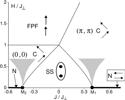
FIG. 1.: Ground states of ${\cal H}$. The arrows denote the mean orientations of the spins in the two layers, for the case where $H$ points vertically upwards; in the SS phase the spins have no definite orientation. The in-plane ordering wavevectors of the $x,y$ components of the spins in the C phase are indicated. The boundaries of the SS phase approach the points $M_{\mu}$ ($\mu=1,2$) as $H/J_{\perp}\sim|w-w_{\mu}|^{\nu}$ where $w\equiv J/J_{\perp}$, $w_{1}=0.398$ (also determined in Refs. [12, 13]), $w_{2}=-0.435$ (also determined in Ref. [14]), and $\nu\approx 0.7$ is the correlation length exponent of the three dimensional classical Heisenberg ferromagnet. There is a Kosterlitz Thouless transition at non-zero $T$ above the C phases, and the result (1) applies above the shaded regions.

We will now discuss phases in Fig. 1 in turn, and also indicate the nature of the quantum transitions between them:
(i) Fully Polarized Ferromagnet (FPF): For large enough $H$, the exact ground state is simply the state with all spins up i.e. in the eigenstate of $\hat{S}_{aiz}$ with eigenvalue $1/2$. The first excited state is a single spin-flip, and its excitation energy can be determined exactly: at momentum $\vec{k}=(k_{x},k_{y})$ it is $\epsilon_{\vec{k}}=H-J_{\perp}-J(2-\cos k_{x}-\cos k_{y})$. For $J>0$ ($J<0$) this has a minimum at $\vec{k}=(\pi,\pi)$ ($\vec{k}=(0,0)$). Stability of the FPF state requires that $\epsilon_{\vec{k}}=\geq 0$, and the point where the minimum energy first vanishes exactly determines the FPF phase boundary shown in Fig. 1. The single spin-flips Bose condense at this boundary, leading to a phase with canted spin order to be described below. This transition is in the universality class of the dilute Bose gas quantum critical point [15] with dynamic exponent $z=2$.
(ii) Spin Singlet (SS): This is the spin singlet quantum paramagnet with no broken symmetries and a gap to all excitations. The exact ground state is known only for $J=0$, when the system decouples into pairs of spins antiferromagnetically coupled by $J_{\perp}$, which therefore form a spin singlet valence bond (see Fig. 1). The ground state for $J\neq 0$ is adiabatically connected to this decoupled state, and its wavefunction can be determined [13] in an expansion in powers of $J/J_{\perp}$. For $H=0$, the lowest excited state is triplet particle, again adiabatically connected to the $J=0$ limit, whose dispersion has been computed [13] in a series in $J/J_{\perp}$. Turning on a nonzero $H$ leads to no change in the wavefunctions, but the energy of the particle changes by $\epsilon_{\vec{k}}\rightarrow\epsilon_{\vec{k}}-mH$, with $m=1,0,-1$ the $S_{z}$ quantum number. As for the FPF phase, the boundary of the SS phase is the line where the minimum excitation energy vanishes. For $J>0$, the boundary is at $H/J_{\perp}=1-2w-(3/2)w^{3}-(3/2)w^{4}+{\cal O}(w^{5})$, with $w\equiv J/J_{\perp}$, while for $J<0$ it is at $H/J_{\perp}=1+2w-(7/4)w^{4}+{\cal O}(w^{5})$. For $H>0$, there is a Bose condensation of the particle at this line, which is in the same universality class as the boundary of the FPF phase, and also leads to the same canted phase. Precisely at $H=0$ (the points $M_{1}$, $M_{2}$ in Fig. 1) the nature of the transition is different, and will be discussed below.
(iii) Canted (C): ${\cal H}$ has a symmetry of rotations about the axis ($z$) of the applied field, and this is broken in this phase. The spin operators have the expectation values $\langle\hat{S}_{1z}\rangle=\langle\hat{S}_{2z}\rangle\neq 0$ and $\langle\hat{S}_{1x,y}\rangle=-\langle\hat{S}_{2x,y}\rangle\neq 0$. The $z$ expectation values are independent of $i$, while the $x,y$ expectation values have staggered (uniform) arrangement on the two sublattices with each layer for $J>0$ ($J<0$). Associated with the broken symmetry, there is linearly dispersing Goldstone mode of spin-wave excitations corresponding to slow rotations of the order parameter in the $x,y$ plane.
(iv) Néel (N): This is reached in the $H=0$ limit of the $C$ phase, when $\langle\hat{S}_{az}\rangle=0$. Now ${\cal H}$ has the full $SU(2)$ spin rotation symmetry, and so the spin expectation values in the $x,y$ plane can actually point along any direction in spin space.

The vicinities of the critical points $M_{1,2}$ are of particular interest in this paper. Here the system is expected [6, 10] to be described by a continuum quantum field theory which can be expressed in terms of a unit length field ${\bf n}(x,\tau)$ ($\tau$ is imaginary time). For $M_{1}$, ${\bf n}\propto\sum_{i\in{\cal N}_{x}}(-1)^{i_{x}+i_{y}}(\hat{\bf S}_{1i}-\hat{\bf S}_{2i})$ and for $M_{2}$, ${\bf n}\propto\sum_{i\in{\cal N}_{x}}(\hat{\bf S}_{1i}-\hat{\bf S}_{2i})$, where ${\cal N}_{x}$ is an averaging neighborhood of $x$. The field theory has the action

$${\cal S}=\frac{c}{2g}\int d^{2}xd\tau\left[(\nabla_{x}{\bf n})^{2}+\frac{1}{c^{2}}\left(\frac{\partial{\bf n}}{\partial\tau}+i{\bf H}\times{\bf n}\right)^{2}\right],$$ (4)

with $c$ a velocity and $g$ a coupling constant which tunes the value of $J/J_{\perp}$. At $H=0$ this theory can be reinterpreted as the real partition function of a three-dimensional classical Heisenberg ferromagnet at non-zero temperature. However no such classical interpretation is possible for $H\neq 0$: notice then that the action is complex (even in imaginary time), as it includes the Berry phase of the precession of the ${\bf n}$ quanta about the applied field. Applying a field at the scale-invariant critical points $M_{1,2}$, we can conclude that all characteristic temperatures will be determined by $H$. Scaling arguments [11], which rely on the fact that ${\bf H}$ appears in ${\cal S}$ as the time component of a $O(3)$ non-Abelian gauge field (which is in turn related to the fact that ${\bf H}$ couples to the conserved total spin), show that $H$ scales as an inverse time; as temperatures also scales as inverse time, we are then lead to (1) for the critical temperature at which the field-induced canted order will disappear.

We turn now to our quantum Monte Carlo results, obtained using the powerful loop algorithm[16] successfully used in recent studies of quantum Heisenberg[17] and XY models[18]. All weights are positive in this basis if we apply the field along the axis of quantization, and the Berry phases have been transformed into the quantization of the spins on the world lines[19]. The loop algorithm slows down severely for $H\neq 0$ [20], as a loop that changes the magnetization by $\Delta M$ picks up a flipping probability $\exp(H\Delta M/T)$; this leads to an exponential increase of the autocorrelation times from $\tau_{\rm int}<1$ to $\tau_{\rm int}\propto\exp(H/T)$. Fortunately it is sufficient to simulate at not too low $T$, where $H/T<4$ and $\tau_{\rm int}<100$, but our system sizes, $L$, are not as large as in earlier $H=0$ studies[17, 18].

We obtained $T_{KT}$ following the method of Harada and Kawashima[18] for the quantum XY model. The spin stiffness, $\rho_{s}$, of the $U(1)$ ordering in the $x-y$ plane was obtained from $\rho_{s}=T\left\langle W_{x}^{2}+W_{y}^{2}\right\rangle/2$, where $W_{x,y}$ are the total winding numbers in the two directions. The improved estimators in Ref. [18] have to be modified, since the flipping probabilities of loops are no longer all equal, and a multi-loop algorithm is necessary. For $L=\infty$, $\rho_{s}$ is finite for $T<T_{KT}$, continuously decreases to the universal value $\rho_{s}(T=T_{KT})=(2/\pi)T_{KT}$ at $T_{KT}$ and is zero for all $T>T_{KT}$. However, for $L$ finite, $\rho_{s}$ is nonzero at all $T$, and is expected to converge to the $L=\infty$ limit with the finite size scaling form at $T=T_{KT}$ [18, 21]:

$$\pi\rho_{s}/2T=1+[2\log(L/L_{0}(T))]^{-1}.$$ (5)

Hence, good estimates for $T_{KT}$ can be obtained by plotting $1/(\pi\rho_{s}/T-2)-\log L$ as a function of $L$. As $L$ is increased this quantity converges to the constant $(-\log L_{0})$ at $T_{KT}$, and diverges to $\pm\infty$ for $T>T_{KT}$ and $T<T_{KT}$ respectively. Our data (a representative example is shown in Fig. 2) are clearly consistent with these expectations.

FIG. 2.: Scaling plot of $1/(\pi\rho_{s}/T-2)-\log L$ versus $L$. This quantity, which diverges to $+\infty$ for $T>T_{KT}$ and to $-\infty$ for $T<T_{KT}$ allows a reliable estimate of $T_{KT}$.

Note that we obtained $L_{0}\approx 5$ to $10$, compared to $L_{0}=0.23$ in the $XY$ model[18]; so we cannot use the more elaborate fitting techniques used in Ref. [18], as we are not deep enough in the asymptotic scaling regime.

FIG. 3.: Spin stiffness $\rho_{s}$ in a magnetic field $H=0.2J$ of ${\cal H}$ for (a) the single layer model ($J_{\perp}=0$) and (b) vertically above the critical point $M_{1}$ of Fig. 1, as a function of $T$ for various $L$. The dashed lines are the lines of universal values at $T_{KT}$: $(\pi/2)\rho_{s}(T_{KT})=T_{KT}$.

First, we checked for a KT transition for the decoupled single-layer case ($J_{\perp}=0$). Our results for $\rho_{s}$ (per layer) are shown in Fig. 3a. We find KT transitions at $T_{KT}/J=0.190(5)$ for $H/J=0.1$ and at $T_{KT}/J=0.215(5)$ for $H/J=0.2$. Surprisingly however, anomalous non-monotonic finite size scaling behavior was found below $T_{KT}$. As can be seen in Fig. 3a, when increasing $L$, first $\rho_{s}$ decreases, then increases again, and is asymptotically expected to decrease again, like in the XY model. A similar anomalous scaling was found in this model by Lavalle et al. [22] for the ground state energy in subspaces of nonzero spin $S\propto L^{2}$.

We now turn to fields above the critical points $M_{1}$ and $M_{2}$. We performed simulations in fields $H/J=0.1$, $0.15$, $0.2$, $0.4$, $0.6$ and $1$. Here no anomalous finite size scaling is observed, as can be seen in Fig. 3b (the $\rho_{s}$ now is the total value, not per layer). We can thus confidently use the finite size scaling analysis to determine $T_{KT}$ as a function of $H$, and show the results in Fig. 4.

FIG. 4.: The critical temperature $T_{KT}$ as a function of field $H$ for the square lattice (isolated layers) and for the antiferromagnetic (AFM) and ferromagnetic (FM) bilayer models close to both critical points.

We fit the results of Fig. 4 $H/|J|\leq 0.2$ to $T_{KT}=a(\delta)+\kappa H$, where the offset $a(\delta)$ accounts for the error in our determination of the positions of $M_{1,2}$. We obtained for the slope $\kappa=0.35(7)$ at $M_{1}$ and $\kappa=0.37(5)$ at $M_{2}$. These numbers agree very well. The error bars are our estimate of strict upper and lower bounds, and not one-sigma confidence intervals. We obtained $a(\delta)\approx 0.01J$, comparable with what the $H=0$, $T=0$ $\rho_{s}$ could be, given the uncertainty of about 0.4% in the determination of the critical points (compare the results for slightly different coupling ratios in Fig. 4).

Corrections to scaling from not being in the continuum limit appear at $H\sim J$ and lead to $T_{KT}=\kappa H(1-bH/|J|)$: these are smaller and were ignored in above fits for $H/|J|\leq 0.2$. Using above estimates for $\kappa$ and $a(\delta)$ and a small correction $b\approx 0.3$ we can however fit all our results up to $H=0.6|J|$. This correction slightly increases our final combined estimate:

$$\kappa\approx 0.38\pm 0.06;$$ (6)

we also recall the leading result in the $\epsilon=3-d$ expansion [6, 10]: $\kappa=\sqrt{33/10\pi^{2}\epsilon}\approx 0.58$.

To conclude, we have obtained a numerical estimate for the universal temperature of a KT transition in the vicinity of a quantum critical point. This universal quantity relies on an underlying interacting quantum field theory with complex Berry phases in $d=2$, and experiments to measure it in bilayer quantum Hall systems will be of considerable interest. Current measurements [2, 9] of $T_{KT}$ are in the vicinity of (1), but more detailed measurements in the shaded region of Fig 1 are necessary, possibly by pressure tuning of the $g$-factor [23].

We thank S. Das Sarma and M. Gelfand for discussions. This research was supported by NSF Grant No DMR 96–23181. The QMC calculations were performed on the Hitachi SR2201 massively parallel computer of the University of Tokyo, using a parallelizing Monte Carlo library in C++ developed by one us[24].

REFERENCES

- [1] Perspectives in Quantum Hall Effects, S. Das Sarma and A. Pinczuk eds, Wiley, New York (1997).
- [2] V. Pellegrini et al., Science 281, Aug 7 (1998).
- [3] J.G.S. Lok et al., cond-mat/9804256.
- [4] A. Sawada et al., Phys. Rev. Lett. 80, 4534 (1998).
- [5] Y.A. Bychkov, S.V. Iordanskii and G.M. Eliashberg, JETP Lett. 33, 143 (1981); C. Kallin and B.I. Halperin, Phys. Rev. B 30, 5655 (1984).
- [6] S. Das Sarma, S. Sachdev and L. Zheng, Phys. Rev. Lett. 79, 917 (1997).
- [7] L. Zheng, R.J. Radtke and S. Das Sarma, Phys. Rev. Lett. 78, 2453 (1997).
- [8] A. Pinczuk et al. Bull. Am. Phys. Soc. 41, 482 (1996); A.S. Plaut, ibid. 41, 590 (1996).
- [9] V. Pellegrini et al. Phys. Rev. Lett. 78, 310 (1997).
- [10] S. Das Sarma, S. Sachdev and L. Zheng, Phys. Rev. B 58, August 15 (1998); cond-mat/9709315.
- [11] S. Sachdev, Z. Phys. B 94, 469 (1994).
- [12] T. Matsuda and K. Hida, J. Phys. Soc. Jpn 59, 2223 (1990); K. Hida, ibid 59, 2230 (1990); A.J. Millis and H. Monien, Phys. Rev. Lett. 70, 2810 (1993); A.W. Sandvik and D.J. Scalapino, ibid 72, 2777 (1994); A.W. Sandvik, A.V. Chubukov and S. Sachdev, Phys. Rev. B 51, 16483 (1995); C.N.A. van Duin and J. Zaanen, Phys. Rev. Lett. 78, 3019 (1997); Zheng Weihong, cond-mat/9701214; M.P. Gelfand, Zheng Weihong, C.J. Hamer and J. Oitmaa, Phys. Rev. B 57, 392 (1998); V.N. Kotov, O. Sushkov, Zheng Weihong and J. Oitmaa, Phys. Rev. Lett. 80, 5790 (1998); K. Hida, cond-mat/9712293; L. Yin, M. Troyer and S. Chakravarty, Europhys. Lett. 44, 559 (1998).
- [13] M.P. Gelfand, Phys. Rev. B 53, 11309 (1996).
- [14] Y. Matsushita et al., J. Phys. Soc. Jpn 66, 3648 (1997).
- [15] S. Sachdev and T. Senthil, Annals of Phys. 251, 76 (1996).
- [16] H. G. Evertz et al. Phys. Rev. Lett. 70, 875 (1993); B. B. Beard and U.-J. Wiese, Phys. Rev. Lett. 77, 5130 (1996).
- [17] M. Troyer et al., Phys. Rev. Lett. 76, 3822 (1996); M. Troyer et al., Phys. Rev. B 55, R6117 (1997); M. Troyer et al., J. Phys. Soc. Jpn. 66, 2957 (1997).
- [18] K. Harada and N. Kawashima, Phys. Rev. B 55, R11949 (1997); cond-mat/9803090.
- [19] For , any basis will have either complex Berry phases or quantized spins. In contrast, for , can be represented by a continuous spin classical ferromagnet in .
- [20] V. A. Kashurnikov et al., cond-mat/9802294.
- [21] H. Weber and P. Minnhagen, Phys. Rev. B 37, 5986(1987).
- [22] C. Lavalle, S. Sorella and A. Parola, cond-mat/9709174.
- [23] D.R. Leadley et al., cond-mat/9805357.
- [24] M. Troyer, B. Ammon and E. Heeb, Lecture Notes in Computer Science (Springer Verlag, in press).