Square vortex lattices for two component superconducting order parameters

Abstract

I investigate the vortex lattice structure of the Ginzburg Landau free energy for a two component order parameter in the weak-coupling clean-limit when the field is along the high symmetry axis in a tetragonal crystal. It is shown that the vortex lattice phase diagram as a function of the Ginzburg Landau free energy parameters includes phases with a hexagonal, centered rectangular, rectangular, and square unit cells. It is also shown that the square vortex lattice has the largest region of stability. The field distribution of the square vortex lattice near $H_{c2}$ is determined and the application of this model to Sr₂RuO₄ is discussed.

The oxide Sr₂RuO₄ has a structure similar to high $T_{c}$ materials and was discovered to be superconducting with a $T_{c}=1.35$ K by Maeno et. al in 1994 [1]. It has been established that this superconductor is not a conventional $s$-wave superconductor: NQR measurements show no indication of a Hebel-Slichter peak in $1/T_{1}T$ [2], $T_{c}$ is strongly suppressed by non-magnetic impurities [3], and tunneling experiments are inconsistent with $s$-wave pairing [4]. More recently there have been two experimental results that shed more light on the nature of the superconducting state. The $\mu$SR experiments of Luke et. al. indicate that the superconducting state breaks time reversal symmetry which implies that the superconducting order parameter must have more than one component [5]. Of the possible representations (REPS) of the $D_{4h}$ point group, the two dimensional (2D) $\Gamma_{5u}$ representation (REP) is the most likely state that exhibits this property. The order parameter in this case has two components $({\eta_{1},\eta_{2}})$ that share the same rotation-inversion symmetry properties as $(k_{x},k_{y})$ [6]. The broken ${\cal T}$ state would then correspond to $(\eta_{1},\eta_{2})\propto(1,i)$. Theoretical arguments supporting a triplet pairing state have been given in Ref. [7]. Given that this material may well be described by such an order parameter, it is of interest to explore further consequences of a two-component order parameter. In an earlier work it was shown that a consequence of the low temperature broken time reversal symmetry state is that the mean field vortex lattice phase diagram will exhibit two vortex lattice phases when the field is along a high symmetry direction in the basal plane [8]. Another important experimental development is the observation of a square vortex lattice in Sr₂RuO₄ by Forgan et. al [9]. Within the context of the orbital dependent superconductivity model for Sr₂RuO₄ the orientation of the square vortex lattice relative to the underlying ionic lattice dictates which of the Ru orbitals exhibit superconductivity [8]. This work focuses on the magnetic field distribution and the structure of the vortex lattice for the field along the $c$-axis for this two-component model.

The free energy for the $\Gamma_{5u}$ representation of the tetragonal point group is given by [6]

$$f= -\alpha|\vec{\eta}|^{2}+\beta_{1}|\vec{\eta}|^{4}/2+\beta_{2}(\eta_{1}\eta_{2}^{*}-\eta_{2}\eta_{1}^{*})^{2}/2+\beta_{3}|\eta_{1}|^{2}|\eta_{2}|^{2}+\kappa_{1}(|\tilde{D}_{x}\eta_{1}|^{2}+|\tilde{D}_{y}\eta_{2}|^{2})$$ (1)

$$+\kappa_{2}(|\tilde{D}_{y}\eta_{1}|^{2}+|\tilde{D}_{x}\eta_{2}|^{2})+\kappa_{5}(|\tilde{D}_{z}\eta_{1}|^{2}+|\tilde{D}_{z}\eta_{2}|^{2})$$ (2)

$$+\kappa_{3}[(\tilde{D}_{x}\eta_{1})(\tilde{D}_{y}\eta_{2})^{*}+h.c.]+\kappa_{4}[(\tilde{D}_{y}\eta_{1})(\tilde{D}_{x}\eta_{2})^{*}+h.c.]+h^{2}/(8\pi).$$ (3)

where $\alpha=\alpha_{0}(T-T_{c})$, $\tilde{D}_{j}=\nabla_{j}-\frac{2ie}{\hbar c}A_{j}$, ${\bf h}=\nabla\times{\bf A}$, and ${\bf A}$ is the vector potential. To simplify the analysis the Ginzburg Landau coefficients are determined within a weak-coupling approximation in the clean limit. The measurements of Mackenzie et. al. of $T_{c}$ as a function of impurity concentration show that the ratio of the mean free path to the zero-temperature coherence length is $>8$ for $T_{c}>1.3$ K [3] indicating that the clean limit should be a reasonable approximation for Sr₂RuO₄. Without an experimental knowledge of the characteristic frequency of the boson responsible for the pairing (presumably ferromagnetic spin fluctuations) it cannot be determined that the weak-coupling limit is appropriate for Sr₂RuO₄. Note that the spin fluctuation theory of Mazin and Singh indicate that $T_{c}/T_{P}\approx 10^{-2}$ where $T_{P}$ is the characteristic paramagnon frequency [11]. This estimate in conjunction with $T_{c}/T_{F}\approx 10^{-4}$ indicates that the weak-coupling approximation is reasonable for Sr₂RuO₄, but further experiments are required to ensure this. Taking for the $\Gamma_{5u}$ REP the gap function described by the pseudo-spin-pairing gap matrix (note that this choice is not unique): $\hat{\Delta}=i[\eta_{1}v_{x}/(\langle v_{x}^{2}\rangle)^{1/2}+\eta_{2}v_{y}/(\langle v_{x}^{2}\rangle)^{1/2}]\sigma_{z}\sigma_{y}$ where the brackets $\langle\rangle$ denote an average over the Fermi surface and $\sigma_{i}$ are the Pauli matrices, writing $\eta_{+}=(\eta_{1}+i\eta_{2})/\sqrt{2}$, $\eta_{-}=(\eta_{1}-i\eta_{2})/\sqrt{2}$, and rotating $(\tilde{D}_{x},\tilde{D}_{y})$ by an angle $\theta$ about the $z$-axis to obtain $(\tilde{D}_{\tilde{x}},\tilde{D}_{\tilde{y}})$, the following dimensionless free energy is found

$$f= -(|\eta_{+}|^{2}+|\eta_{-}|^{2})+(|\eta_{+}|^{4}+|\eta_{-}|^{4})/2+2|\eta_{+}|^{2}|\eta_{-}|^{2}+\nu[(\eta_{-}\eta_{+}^{*})^{2}/2+(\eta_{-}^{*}\eta_{+})^{2}]$$ (4)

$$+|D_{\tilde{x}}\eta_{+}|^{2}+|D_{\tilde{y}}\eta_{-}|^{2}+|D_{\tilde{x}}\eta_{-}|^{2}+|D_{\tilde{y}}\eta_{+}|^{2}$$ (5)

$$+(e^{i2\theta}+\nu e^{-i2\theta})[(D_{\tilde{x}}\eta_{+})(D_{\tilde{x}}\eta_{-})^{*}-(D_{\tilde{y}}\eta_{+})(D_{\tilde{y}}\eta_{-})^{*}]/2$$ (6)

$$+(e^{-i2\theta}+\nu e^{i2\theta)})[(D_{\tilde{x}}\eta_{-})(D_{\tilde{x}}\eta_{+})^{*}-(D_{\tilde{y}}\eta_{-})(D_{\tilde{y}}\eta_{+})^{*}]/2$$ (7)

$$+I(e^{-i2\theta}-\nu e^{i2\theta})[(D_{\tilde{x}}\eta_{-})(D_{\tilde{y}}\eta_{+})^{*}+(D_{\tilde{y}}\eta_{-})(D_{\tilde{x}}\eta_{+})^{*}]/2$$ (8)

$$-I(e^{i2\theta}-\nu e^{-i2\theta})[(D_{\tilde{x}}\eta_{+})(D_{\tilde{y}}\eta_{-})^{*}+(D_{\tilde{y}}\eta_{+})(D_{\tilde{x}}\eta_{-})^{*}]/2+\tilde{\kappa}_{5}(|D_{z}\eta_{+}|^{2}+|D_{z}\eta_{-}|^{2})+h^{2},$$ (9)

where $h=\nabla\times{\bf A}$, $D_{\nu}=\nabla_{\nu}/\kappa-iA_{\nu}$, $f$ is in units $B_{c}^{2}/(4\pi)$, lengths are in units $\lambda=[\hbar^{2}c^{2}\beta_{1}/(32e^{2}\kappa_{1}\alpha\pi)]^{1/2}$, $\tilde{\kappa}_{5}=2\kappa_{5}/\kappa_{12}$, $\kappa_{12}=\kappa_{1}+\kappa_{2}=4\kappa_{1}/(3+\nu)$, $\nu=(\langle v_{x}^{4}\rangle-3\langle v_{x}^{2}v_{y}^{2}\rangle)/(\langle v_{x}^{4}\rangle+\langle v_{x}^{2}v_{y}^{2}\rangle)$, $h$ is in units $\sqrt{2}B_{c}=\Phi_{0}/(2\pi\lambda\zeta)$ (here $B_{c}$ has been chosen to represent the thermodynamic critical field), $\alpha=\alpha_{0}(T-T_{c})$, $\xi=(\kappa_{12}/2\alpha)^{1/2}$, and $\kappa=\lambda/\xi$. The parameter $\nu$ (note $|\nu|\leq 1$) gives a measure of the square anisotropy of the Fermi surface. For a cylindrical Fermi surface $\nu=0$ and for a square Fermi surface $|\nu|=1$. It is easy to verify that in zero-field $(\eta_{1},\eta_{2})\propto(1,i)$ is the stable ground state for $|\nu|\leq 1$.

For the magnetic field along the $c$-axis the ground state is found by setting $D_{z}=0$. Writing $\Pi_{+}=\sqrt{\kappa}(iD_{\tilde{x}}+D_{\tilde{y}})/\sqrt{2H}$ and $\Pi_{-}=\sqrt{\kappa}(iD_{\tilde{x}}-D_{\tilde{y}})/\sqrt{2H}$, minimizing the quadratic portion of Eq. 4 with respect to $\eta_{+}$ and $\eta_{-}$ yields

$$\kappa\pmatrix{\eta_{+}\cr\eta_{-}}=H\pmatrix{1+2N&e^{-2i\theta}\Pi_{+}^{2}+\nu e^{2i\theta}\Pi_{-}^{2}\cr e^{2i\theta}\Pi_{-}^{2}+\nu e^{-2i\theta}\Pi_{+}^{2}&1+2N}\pmatrix{\eta_{+}\cr\eta_{-}}.$$ (10)

where $N=\Pi_{+}\Pi_{-}$. The maximum value of the externally applied field $H$ that allows a non-zero solution for $(\eta_{+},\eta_{-})$ yields the upper critical field $H_{c_{2}}$. At $H=H_{c2}$ the vector potential is that for a spatially uniform field ${\bf A}=(0,Hx,0)$. Expanding $(\eta_{+},\eta_{-})$ in terms of the eigenstates of $N$ (Landau levels) up to $N=32$ and diagonalizing the resulting matrix yields the result for $e_{H}=\kappa/H_{c_{2}}$ shown as a function of $\nu$ in Fig. 1.

FIG. 1.: $e_{H}=\kappa/H_{c_{2}}$ as a function of $\nu$.

The form of the eigenstate of the $H_{c_{2}}$ solution is found to be $\eta_{+}({\bf r})=\sum_{n\geq 0}a_{4n+2}\phi_{4n+2}({\bf r})$ and $\eta_{-}({\bf r})=\sum_{n\geq 0}a_{4n}\phi_{4n}({\bf r})$ where $\phi_{n}({\bf r})$ are the harmonic oscillator wave functions (Landau levels). As is well known these wave functions have a large degeneracy, and the form of the vortex lattice is found by including the nonlinear terms of the Ginzburg Landau equations perturbatively to break this degeneracy. Following the procedure of Abrikosov, the average Gibbs free energy density is found to be (a derivation of this result for unconventional superconductors can be found in Ref. [12] and for a mixed $d$ and $s$-wave order parameter in Ref. [13])

$$\overline{g}=-H^{2}-\frac{(H_{c_{2}}-H)^{2}}{(2\tilde{\kappa}^{2}-1)\beta_{A}}$$ (11)

where

$$\beta_{A}=\frac{\overline{h_{s}^{2}}}{(\overline{h_{s}})^{2}},$$ (12)

$$2\tilde{\kappa}^{2}=\frac{\overline{f_{4}}}{\overline{h_{s}^{2}}}$$ (13)

$f_{4}$ is the fourth order homogeneous free energy, $h_{s}$ is the field (along the $c$-axis) induced by the supercurrent, and the over-bar denotes a spatial average. The form of the vortex lattice is found by minimizing $(2\tilde{\kappa}^{2}-1)\beta_{A}$. To do this $h_{s}$ must be found. By minimizing the Ginzburg Landau free energy with respect to the vector potential the following relation is found for $h_{s}$

$$j_{+}\equiv\frac{\partial h_{s}}{\partial y}-i\frac{\partial h_{s}}{\partial x}= \eta_{+}^{*}(\Pi_{-}\eta_{+})+\eta_{+}(\Pi_{+}\eta_{+})^{*}+\eta_{-}^{*}(\Pi_{-}\eta_{-})+\eta_{-}(\Pi_{+}\eta_{-})^{*}$$ (14)

$$+e^{i2\theta}[\eta_{-}^{*}(\Pi_{+}\eta_{+})+\eta_{+}(\Pi_{-}\eta_{-})^{*}]+\nu e^{i2\theta}[\eta_{+}^{*}(\Pi_{+}\eta_{-})+\eta_{-}(\Pi_{-}\eta_{+})^{*}]$$ (15)

$$j_{-}\equiv\frac{\partial h_{s}}{\partial y}+i\frac{\partial h_{s}}{\partial x}= \eta_{+}(\Pi_{-}\eta_{+})^{*}+\eta_{+}^{*}(\Pi_{+}\eta_{+})+\eta_{-}(\Pi_{-}\eta_{-})^{*}+\eta_{-}^{*}(\Pi_{+}\eta_{-})$$ (16)

$$+e^{-i2\theta}[\eta_{-}(\Pi_{+}\eta_{+})^{*}+\eta_{+}^{*}(\Pi_{-}\eta_{-})]+\nu e^{-i2\theta}[\eta_{+}(\Pi_{+}\eta_{-})^{*}+\eta_{-}^{*}(\Pi_{-}\eta_{+})]$$ (17)

Near $H_{c_{2}}$ the field $h_{s}$ is found by substituting the vector potential for the homogeneous field and the order parameter solution near $H_{c_{2}}$ into the right hand side of Eq. 14. Writing the left hand side of Eq. 14 as $j_{i}=\sum_{n,m}(j_{i})_{n,m}\phi_{n}\phi_{m}^{*}$ and writing $h_{s}=\sum_{n,m}h_{n,m}\phi_{n}\phi_{m}^{*}$ yields (see Ref [14])

$$h_{l,l}= \sum_{n=l}^{\infty}(j_{+})_{n+1,n}/\sqrt{n+1}$$ (18)

$$h_{l,p}= [\sqrt{l}(j_{+})_{l-1,p}-\sqrt{p}(j_{+})_{p-1,l}^{*}]/(p-l) \hphantom{abcdefghijk}l\neq p.$$ (19)

The form of $\beta_{A}$ and $\tilde{\kappa}$ will therefore be determined by terms of the type $\overline{\phi_{n}({\bf r})\phi_{m}^{*}({\bf r})\phi_{p}({\bf r})\phi_{l}^{*}({\bf r})}$. To evaluate such terms I make the assumption that the vortex lattice unit cell contains one flux quantum. The shape of the unit cell is kept arbitrary and the convention introduced by Saint-James et. al [15] to describe the unit cell is used. The lattice geometry is depicted in Fig. 2.

FIG. 2.: The vortex lattice unit cell

The lattice vectors are ${\bf a}_{1}=a(1,0)$ and ${\bf a}_{2}=b(\cos\alpha,\sin\alpha)$ with the single flux quantum constraint $ab\sin\alpha=2\pi$ where $a$ and $b$ are in units $l_{H}=2\pi\sqrt{\lambda\xi/H}$. This assumption allows the functions $\phi_{n}$ to be written as [12]

$$\phi_{n}({\bf r})=2^{-n/2}\pi^{-1/4}(n!)^{-1/2}\sum_{m}c_{m}e^{i2\pi(m-1/2)x/a}e^{-(y-y_{m})^{2}/2}H_{n}(y-y_{m})$$ (20)

where $c_{n}=e^{i\pi n(\rho+1-n\rho)}$, $y_{n}=(n-1/2)\sqrt{2\pi\sigma}$, $\sigma=(b/a)\sin\alpha$, $\rho=(b/a)\cos\alpha$, and $H_{n}$ are the Hermite polynomials. To evaluate $\beta_{A}$ and $\tilde{\kappa}$ it is useful to express the spatial averages in terms of a sum over the reciprocal lattice of the vortex lattice. The reciprocal lattice is given by ${\bf G}=l_{1}{\bf k}_{1}+l_{2}{\bf k}_{2}$ where ${\bf k}_{1}=\frac{2\pi}{a\sin\alpha}(\sin\alpha,-\cos\alpha)$ ${\bf k}_{2}=\frac{2\pi}{b\sin\alpha}(1,0)$. The general form of $\beta_{A}$ becomes

$$\beta_{A}=\frac{\sum_{n,m,p,l}a_{n,m,p,l}\sum_{l_{1},l_{2}}\langle\phi_{n}\phi_{m}^{*}\rangle_{l_{1},l_{2}}\langle\phi_{p}\phi_{l}^{*}\rangle_{-l_{1},-l_{2}}}{[\sum_{n}a_{n}\langle|\phi_{n}|^{2}\rangle_{0,0}]^{2}}$$ (21)

where the coefficients $a_{n,m,p,l}$ and $a_{n}$ are determined by $f_{4}$, $h_{s}$, and the form of the eigenfunction near $H_{c_{2}}^{c}$, $\langle f\rangle_{l_{1},l_{2}}=(ab\sin\alpha)^{-1}\int_{uc}e^{-i{\bf G}\cdot{\bf r}}f({\bf r})$, and $uc$ denotes the unit cell. The following relation makes this formulation for determining $\beta_{A}$ and $\tilde{\kappa}$ useful (found using the addition theorem for Hermite polynomials)

$$\langle\phi_{p}\phi_{m}^{*}\rangle_{l_{1},l_{2}}=\frac{2^{-(m+p)/2}}{\sqrt{p!m!}}\langle|\phi_{0}|^{2}\rangle_{l_{1},l_{2}}\sum_{r=0}^{p}\sum_{s=0}^{m}\frac{C_{r,s}H_{p-r}[-z_{l_{1},l_{2}}]H_{m-s}[z_{l_{1},l_{2}}^{*}]}{(p-r)!(m-s)!}$$ (22)

where

$$C_{r,s}=\sum_{l=0}^{[r/2]}\sum_{p=0}^{[s/2]}(-1)^{l+p}\frac{(r+s-2l-2p)!2^{-l-p+(r+s)/2}}{(r-2l)!(s-2p)!l!p![(r+s)/2-l-p]!},$$ (23)

$z_{l_{1},l_{2}}=\sqrt{\pi}[l_{1}\sqrt{\sigma}+i(l_{2}-\rho l_{1})/\sqrt{\sigma}]$, and

$$\langle|\phi_{0}|^{2}\rangle_{l_{1},l_{2}}=\frac{\sqrt{\pi}}{b\sin\alpha}e^{i\pi(l_{1}+l_{2}+l_{1}l_{2})}e^{-\pi\sigma l_{1}^{2}/2}e^{-\pi(l_{2}-l_{1}\rho)^{2}/2\sigma}.$$ (24)

The following relation is also useful

$$\langle\phi_{p}\phi_{0}^{*}\rangle_{l_{1},l_{2}}=[\sqrt{2}z_{l_{1},l_{2}}]^{p}\langle|\phi_{0}|^{2}\rangle_{l_{1},l_{2}}.$$ (25)

The relations 11-14 are straightforward to implement numerically.

In the analysis of the form of the vortex lattice the parameter $\nu$ was considered to lowest order in perturbation theory (recall that $|\nu|\leq 1$ so that $\nu$ provides a natural expansion parameter). The limit $\nu=0$ was considered by Zhitomirsky who analytically found the ground state eigenvector near $H_{c_{2}}$ [16]. The solution of the order parameter to first order in $\nu$ is

$$(\eta_{+},\eta_{-})=[\phi_{0}+b_{4}\nu e^{-i4\theta}\phi_{4},-e^{i2\theta}(\epsilon\phi_{2}+b_{6}\nu e^{-i4\theta}\phi_{6})]$$ (26)

where $\epsilon=\sqrt{3}-\sqrt{2}\approx 0.31784$, $b_{4}=2\sqrt{3}\epsilon(10+\sqrt{6})/(36+16\sqrt{6})\approx 0.18230$, and $b_{6}=\sqrt{30}b_{4}/(10+\sqrt{6})\approx 0.080203$. Substituting this solution for the eigenstate near $H_{c_{2}}$ into the Eq. 6 yields the coefficients

$$(j_{+})_{0,1}= 1-\sqrt{2}\epsilon$$ (27)

$$(j_{+})_{0,5}= e^{i4\theta}\nu(\sqrt{5}b_{4}-\sqrt{6}b_{6})$$ (28)

$$(j_{+})_{1,2}= \sqrt{2}\epsilon^{2}-\epsilon$$ (29)

$$(j_{+})_{1,6}= e^{i4\theta}b_{6}\nu(\sqrt{2}\epsilon-1)$$ (30)

$$(j_{+})_{2,3}= \sqrt{3}\epsilon^{2}$$ (31)

$$(j_{+})_{2,7}= e^{i4\theta}\sqrt{7}\epsilon b_{6}\nu$$ (32)

$$(j_{+})_{3,0}= e^{i4\theta}\nu(2b_{4}-\sqrt{3}\epsilon)$$ (33)

$$(j_{+})_{4,1}= e^{-i4\theta}\nu b_{4}(1-\sqrt{2}\epsilon)$$ (34)

$$(j_{+})_{5,2}= e^{-i4\theta}\epsilon\nu(\sqrt{6}b_{6}-\sqrt{5}b_{4})$$ (35)

$$(j_{+})_{6,3}= e^{-i4\theta}b_{6}\nu\sqrt{3}\epsilon$$ (36)

Application of Eq. 18 yields

$$h_{s}= \frac{-1}{2\kappa}[(1-3/\sqrt{2}\epsilon+2\epsilon^{2})|\phi_{0}|^{2}+(2\epsilon^{2}-\epsilon/\sqrt{2})|\phi_{1}|^{2}+\epsilon^{2}|\phi_{2}|^{2}$$ (37)

$$+\nu[(\sqrt{10}\epsilon b_{4}/4-\sqrt{6}b_{6}/4)(e^{i4\theta}\phi_{1}^{*}\phi_{5}+e^{-i4\theta}\phi_{5}^{*}\phi_{1})$$ (38)

$$+(\sqrt{30}\epsilon b_{4}/4-\epsilon b_{6}-\sqrt{2}b_{6}/4)(e^{i4\theta}\phi_{2}^{*}\phi_{6}+e^{-i4\theta}\phi_{6}^{*}\phi_{2})$$ (39)

$$+(\sqrt{3}\epsilon/2-b_{4})(e^{i4\theta}\phi_{4}^{*}\phi_{0}+e^{-i4\theta}\phi_{0}^{*}\phi_{4})].$$ (40)

Using this expression for $h_{s}$, $(2\tilde{\kappa}^{2}-1)\beta_{A}$ should be minimized with respect to $\theta,\sigma,$ and $\rho$ to find the form of the vortex lattice. It can be proven when $\nu>0$ ($\nu<0$) $(2\tilde{\kappa}^{2}-1)\beta_{A}$ can be minimized for $\theta=\pi/4$ ($\theta=0$). For $\nu=0$, $(2\tilde{\kappa}^{2}-1)\beta_{A}$ is independent of $\theta$. This is to be expected since $\nu=0$ corresponds to a cylindrically symmetric Fermi surface. It is also found that $\tilde{\kappa}$ varies weakly ($\approx 0.01$) for the different vortex lattice structures studied in this article (such behavior is also present for mixed $d$ and $s$-wave order parameters [13]). While this variation is small it determines the form of the vortex lattice in the region of $\tilde{\kappa}\approx 1/\sqrt{2}$ and at small $\kappa$ the vortex lattice phase diagram becomes quite rich.

The form of the vortex lattice found in the large $\kappa$ limit agrees with that found under more restrictive assumptions in Ref. [8]. In this limit the lattice structure depends upon $\nu$. The behavior of the vortex lattice as a function of $\nu$ is similar to the behavior as a function of temperature found for borocarbide [17] and $d$-wave [18, 13] superconductors. For $\nu=0$ a hexagonal lattice is found. As $|\nu|$ increases the lattice deforms continuously until $|\nu|=0.0114$. For $0<|\nu|<0.0114$ the vortex lattice is a centered rectangular lattice as shown in Fig.3 (which can be described by $\theta=\pi/4-\alpha$ and $\rho=\cos\alpha$ and $\sigma=\sin\alpha$ where $\pi/3<\alpha<\pi/2$, $\alpha=\pi/3$ corresponds to the hexagonal lattice and $\alpha=\pi/2$ to the square lattice). For $|\nu|\geq 0.0114$ the vortex lattice is square. If $\nu\geq 0.0114$ the vortex lattice is rotated $\pi/4$ with respect to the underlying crystal lattice while for $\nu\leq-0.0114$ the vortex lattice is aligned with the underlying crystal lattice.

As mentioned above when $\kappa$ becomes sufficiently small the vortex lattice phase diagram becomes richer. Fig. 3 shows the region of stability for the three vortex lattice states that were found to be stable. In addition to the two phases described above a third phase appears for small $\kappa$. The vortex lattice for this phase has a rectangular unit cell and is described by $\rho=0$ and $\sigma=b/a$. This phase is stable because $\tilde{\kappa}$ is smaller for this phase than for both the square and hexagonal lattices. For a cylindrically symmetric Fermi surface ($\nu=0$) and $\kappa<0.75$ the hexagonal vortex lattice is no longer the stable structure. This arises because $\tilde{\kappa}$ is in a local maximum for the hexagonal lattice.

FIG. 3.: The vortex lattice phase diagram as a function of the Ginzburg-Landau ratio $\kappa$ and the square anisotropy parameter $\nu$. The phase diagram is the same for $\nu<0$. For $\nu>0$ ($\nu<0$) the square vortex lattice is rotated $\pi/4$ (0) with respect to the underlying crystal lattice.

The Type I to Type II transition can also be determined and it is not given by $\tilde{\kappa}=1/\sqrt{2}$ but by $H_{c_{2}}=H_{c}$ (which corresponds to $\kappa=\epsilon\sqrt{3/2}$ up to corrections that are second order in $\nu$). For a conventional superconductor $\tilde{\kappa}=1/\sqrt{2}$ and $H_{c_{2}}=H_{c}$ are equivalent. Here it is found that the $\kappa$ for which $\tilde{\kappa}=1/\sqrt{2}$ is less than $\kappa=\epsilon\sqrt{3/2}$ for all lattice structures studied. An analysis of the Gibbs energies indicates that the Meissner state is the stable phase for $H$ near $H_{c_{2}}$ when $\kappa<\epsilon\sqrt{3/2}$.

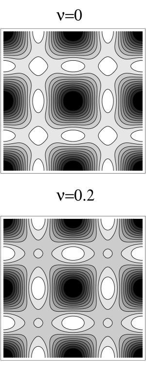
FIG. 4.: Contour plots of the induced magnetic field $h_{s}$ for a square vortex lattice with $\nu=0$ (top) and $\nu=0.2$ (bottom). The contours from darkest to lightest correspond to $\kappa h_{s}=-0.42\rightarrow-0.042$ in units $0.042$.

Clearly the square vortex lattice has the largest region of stability in Fig 3. To further investigate the square vortex lattice the spatial variation of the magnetic field as given by Eq. 37 is determined. This is shown in Fig. 4 for $\nu=0$ and for $\nu=0.2$. The induced field $h_{s}$ has (in addition to a global maximum and a global minimum) a local minimum and a saddle point. Fig. 5 shows the field distribution for these two values of $\nu$ as determined from

$$P(h)=\frac{\int d^{2}r\delta[h-h({\bf r})]}{\int d^{2}r}.$$ (41)

The peak in $P(h)$ is due to the saddle point in the spatial dependence of $h_{s}$. As $\nu$ increases the saddle point value of $h_{s}$ moves away from the minimum value of $h_{s}$ resulting in a larger ’shoulder’ in $P(h)$ as $\nu$ increases.

Now I turn to an application of these results to Sr₂RuO₄. This requires a determination of the parameters $\nu$ and $\kappa$. The value of $\kappa$ as defined above is given by

$$\kappa=\frac{e_{H}H_{c_{2}}}{\sqrt{2}H_{c}},$$ (42)

where $e_{H}$ is given in Fig. 1 and $H_{c}$ ($H_{c_{2}}$) correspond to the measured critical (upper critical) field [note that the above choice of $\kappa$ and $\xi$ also implies $H_{c_{2}}=\Phi_{0}/(2e_{H}\pi\xi^{2})$]. In principle the values for $H_{c_{2}}$ and $H_{c}$ given in Ref. [20] can be used to estimate $\kappa$, however the sample used had a $T_{c}=0.9$ K which indicates that impurities cannot be neglected (since $T_{c}^{max}\approx 1.5$ K) so that the clean-limit approximation used here is not valid. Until measurements on cleaner samples become available these measurements will be used to estimate $\kappa$. Using the values of $H_{c_{2}}$ and $H_{c}$ given in Ref. [20] yields $\kappa=1.2e_{H}<0.7$. This implies that either the square or the orthorhombic vortex lattices will occur depending on the value of $\nu$.

FIG. 5.: Field distribution $P(h)$ near $H_{c_{2}}$ for a square vortex lattice with $\nu=0$ and $\nu=0.2$

To determine the value of $\nu$ experimentally the anisotropy of the upper critical field in the basal plane can be used [21, 8]

$$\frac{H_{c_{2}}({\bf a})}{H_{c_{2}}({\bf a}+{\bf b})}=\frac{1-\nu}{1+\nu}.$$ (43)

where $H_{c_{2}}({\bf a})$ [$H_{c_{2}}({\bf a}+{\bf b})$] is the upper critical field for the field along ${\bf a}$ [${\bf a}+{\bf b}$] measured at $T_{c}$. This anisotropy has not yet been determined so that a microscopic model must be used to estimate $\nu$. LDA band structure calculations [22, 23] reveal that the density of states near the Fermi surface is due mainly to the four Ru $4d$ electrons in the $t_{2g}$ orbitals. There is a strong hybridization of these orbitals with the O $2p$ orbitals giving rise to antibonding $\pi^{*}$ bands. The resulting bands have three quasi-2D Fermi surface sheets labeled $\alpha,\beta,$ and $\gamma$ (see Ref. [24]). The $\alpha$ and $\beta$ sheets consist of $\{xz,yz\}$ Wannier functions and the $\gamma$ sheet of $xy$ Wannier functions. In general $\nu$ is not given by a simple average over all the sheets of the Fermi surface. A knowledge of the pair scattering amplitude on each sheet and between the sheets is required to determine $\nu$ [10, 11]. It has been shown that the pair scattering amplitude between the $\gamma$ and the $\{\alpha,\beta\}$ sheets of the Fermi surface is expected to be small relative to the intra-sheet pair scattering amplitudes if Sr₂RuO₄ is not an isotropic $s$-wave superconductor [10]. This forms the basis for the model of orbital dependent superconductivity in which, to account for the large residual density of states observed in the superconducting state, it has been proposed that either the $xy$ or the $\{xz,yz\}$ Wannier functions exhibit superconducting order. This model implies that that there are two possible values of $\nu$; one for the $\gamma$ sheet ($\nu_{xy}$) and one for an average over the $\{\alpha,\beta\}$ sheets ($\nu_{xz,yz}$). Using the following tight binding dispersions

$$\epsilon_{\gamma}= \epsilon_{\gamma}^{0}-2t_{\gamma}(\cos k_{x}+\cos k_{y})-4\tilde{t}_{\gamma}\cos k_{x}\cos k_{y}$$ (44)

$$\epsilon_{\alpha,\beta}= \epsilon_{\alpha,\beta}^{0}-2t_{\alpha,\beta}(\cos k_{x}+\cos k_{y})\pm\sqrt{4t_{\alpha,\beta}^{2}(\cos k_{x}-\cos k_{y})^{2}+16\tilde{t}_{\alpha,\beta}^{2}\sin^{2}k_{x}\sin^{2}k_{y}}$$ (45)

and using the tight binding values of Ref. [11] for the $\gamma$ sheet $(\epsilon_{\gamma}^{0},t_{\gamma},\tilde{t}_{\gamma})=(-0.4,0.4,0.12)$ and the values $(\epsilon_{\alpha,\beta}^{0},t_{\alpha,\beta},\tilde{t}_{\alpha,\beta})=(-0.3,0.25,0.075)$ for the $\{\alpha,\beta\}$ sheets yields $\nu_{xy}=-0.6$ and $\nu_{xz,yz}=0.6$. These values of $\nu$ seem too large since they imply an anisotropy of a factor of 4 in $H_{c_{2}}({\bf a})/H_{c_{2}}({\bf a}+{\bf b})$. However $\nu$ depends strongly upon the tight binding parameters used, for example taking $(\epsilon_{\gamma}^{0},t_{\gamma},\tilde{t}_{\gamma})=(-0.52,0.4,0.16)$ yields $\nu_{xy}=-0.08$. The qualitative result that $\nu_{xy}<0$ and $\nu_{xz,yz}>0$ is robust. Physically $\nu_{xy}<0$ because of the proximity of the $\gamma$ Fermi surface sheet to a Van Hove singularity and $\nu_{xz,yz}>0$ due to the quasi 1D nature of the $\{\alpha,\beta\}$ surfaces [22, 23]. Assuming $|\nu|<0.2$ implies $\kappa\approx 0.7$ in which case there will be a square vortex lattice that is rotated $\pi/4$ (0) with respect to the underlying crystal lattice if the pairing occurs on the $\{\alpha,\beta\}$ ($\gamma$) Fermi sheets. It is encouraging that Forgan et. al have observed a square vortex lattice in Sr₂RuO₄ [9]. Further experimental studies of the vortex lattice should provide useful information as to the nature of the superconducting phase.

In conclusion a Ginzburg Landau theory for a two component order parameter representation of the tetragonal point group has been examined with a magnetic field applied along the $c$-axis. The vortex lattice phase diagram near $H_{c_{2}}$ was found to be rich with a square vortex lattice occupying most of the parameter space. The field distribution of the square vortex lattice was determined yielding predictions for $\mu$SR measurements. Finally, the application of this model to Sr₂RuO₄ indicates that a square vortex lattice is expected to appear. The orientation of the square vortex lattice with respect to the underlying crystal lattice yields information as to which of the Ru 4$d$ orbitals are relevant to the superconducting state.

I acknowledge support from the Natural Sciences and Engineering Research Council of Canada and the Zentrum for Theoretische Physik. I wish to thank E.M. Forgan, R. Heeb, G. Luke, A. Mackenzie, Y. Maeno, T.M. Rice, and M. Sigrist for useful discussions.

REFERENCES

• [1] Y. Maeno, H. Hashimoto, K.Yoshida,S.Nishizaki, T. Fujita, J.G. Bednorz, and F. Lichtenberg, Nature 372, 532 (1994).
• [2] K. Ishida, Y.Kitaoka, K. Asayama, S.Ikeda, and T. Fujita, Phys. Rev. B 56, 505 (1997).
• [3] A.P. Mackenzie, R.K.W. Haselwimmer, A.W. Tyler, G.G Lonzarich, Y. Mori, S. Nishizaki, and Y. Maeno, Phys. Rev. Lett. 80, 161 (1998).
• [4] R. Jin, Yu. Zadorozhny, Y. Liu, Y. Mori, Y. Maeno, D.G. Schlom, and F. Lichtenberg, J. Chem. Phys. of Solids, in press.
• [5] G.M. Luke, et. al, to be published
• [6] M. Sigrist and K. Ueda, Rev. Mod. Phys. 63, 239 (1991).
• [7] T.M. Rice and M. Sigrist, J. Phys.: Condens. Matter 7, L643 (1995).
• [8] D.F. Agterberg, Phys. Rev. Lett. 80, 5184 (1998).
• [9] E.M. Forgan, et. al., to be published.
• [10] D.F. Agterberg, T.M. Rice, and M. Sigrist, Phys. Rev. Lett. 78, 3374 (1997).
• [11] I.I. Mazin and D.J. Singh, Phys. Rev. Lett. 79, 733 (1997).
• [12] I.A. Luk’yanchuk and M.E. Zhitomirsky, Supercond. Rev. 1, 207 (1995).
• [13] M. Franz, C. Kallin, P.I. Soininen, A.J. Berlinsky, and A.L. Fetter, Phys. Rev. B 53, 5795 (1996).
• [14] K. Takanaka, Prog. Theor. Phys. 46, 1301 (1971).
• [15] D. Saint-James, G. Sarma, and E.J. Thomas, Type II Superconductivity (Pergamon Press, New York, 1969).
• [16] M.E. Zhitomirskii, JEPT Lett. 49, 378 (1989).
• [17] Y. De Wilde, M. Iavarone, U. Welp, V. Metlushko, A.E. Koshelev, I. Aranson, G.W. Crabtree, and P.C. Canfield, Phys. Rev. Lett. 78, 4273 (1997).
• [18] M. Ichioka, N. Enomoto, and K. Machida, J. Phys. Soc. Jpn. 66, 3928 (1997).
• [19] R. Heeb et. al, in preparation.
• [20] K. Yoshida, Y. Maeno, S. Nishizaki, and T. Fujita, J. Phys. Soc. Jpn. 65, 2220 (1996).
• [21] L.I. Burlachkov, Sov. Phys. JEPT 62, 800 (1985).
• [22] T. Oguchi, Phys. Rev. B 51, 1385 (1995).
• [23] D.J. Singh, Phys. Rev. B 52, 1358 (1995).
• [24] A.P Mackenzie, S.R. Julian, A.J. Diver, G.G. Lonzarich, Y. Maeno, S.Nishizaki, and T. Fujita, Phys. Rev. Lett. 76, 3786 (1996).