Breakdown of the Universality Hypothesis in Directed Abelian Sandpile Models

Abstract

We show that in a broad class of directed abelian sandpile models that had been expected to have the same exponents as the Dhar-Ramaswamy model, the avalanche exponent depends upon the details of the interaction, calling into question the general existence of universality classes in self organized critical models.

The existence of universality classes in systems exhibiting self-organized critical behaviour(SOC) is expected on the basis of the similarity of the SOC state to the critical state of equilibrium systems. The particular physical constraints that might determine these classes are, however, very much an open question, but they are thought to resemble the universality classes of equilibrium systems, at least as far as symmettry and dimensionality are concerned. In one dimension, it was shown recently by Paczuski and Boettcher [1] that a model for rice piles and another for interface depinning were in the same universality class, and they conjectured that the Burridge-Knopoff model [2] was contained there as well. Subsequently, Cule and Hwa[3] described a related model that was in the same universality class. A classification scheme for 2-dimensional abelian sandpile models was suggested by Ben-Hur and Biham[4]. In their paper, models were classified according to the ”sand current” ,$\vec{J}$, which resulted when an unstable site was toppled. Models with $\vec{J}=0$ and $\vec{J}\not=0$ were said to be in the ”nondirected” and ”directed” universality classes respectively, and a distinction was made between those that were nondirected only on average. Dhar and Ramaswamy[5](DR) had earlier presented an exact solution for a directed model in two dimensions, and had shown numerically that a closely related directed model had the same exponents. Ben-hur and Biham described having run a third model with the same exponents. However, in their simulations, only models with nearest neighbor interactions were considered. Our investigations of longer (but still finite) range interactions in directed models show a continuous variation of exponent values ranging from those of the exactly solvable nearest neighbor model of DR to that of an exactly solvable infinite range interaction model that we introduce here.

No simple classification is apparent in these models, with exponents depending on the details of the interaction, as well as the range. While it is not unexpected that universality classes in SOC would be more complex than those in equilibrium models, this finding calls into question the idea of using universality ideas to describe these models at all, at least in two dimensions.

Since the variation in exponents is not large(2.33-2.5), we introduce a simulation method which exploits the properties of a subclass of the directed models to greatly reduce the deviation from power law behaviour seen in the simulations as a result of finite system sizes. This allows more accurate determination of scaling exponents from relatively small system sizes. We emphasize, however, that the standard methods for obtaining the exponents yield the same results.

To fix notation, we define a sandpile model by three variable aspects.

  lattice:

In two dimensions the model dynamics occur on a $MxN$ lattice $\mathcal{L}_{MN}$ composed of $d=MN$ sites where sand can build up. This lattice is embedded in an infinite lattice of sites which absorb all sand which fall on them. The state of the system at any given time is a $d$ dimensional integer valued vector whose components represent the height of individual sites.

  critical height:

The critical height $h_{c}$ is the maximum amount of sand which can sit on a site and not topple. If a site has more than $h_{c}$ grains it is said to be unstable and will topple.

  toppling rule:

The toppling (or relaxation) rule determines how sand is removed from an unstable site $i$ and redistributed to sites in some predetermined neighborhood ,${\mathcal{N}}_{i}$, of $i$.

One then defines the set of toppling vectors, {$\vec{T_{j}}$} ,where the subscript corresponds to one of the $d$ lattice sites. The unstable site $i$ with $h_{c}+1$ or more grains is toppled by subtracting the vector $\vec{T}_{i}$ from the state vector. The $s^{th}$ component of $\vec{T_{i}}$ is defined as

$$[\vec{T}_{i}]_{s}=\left\{\begin{array}[]{ll}h_{c}+1&\mbox{if $s=i$}\\ -f_{i}(s)&\mbox{$s\not=i$}\par\end{array}\right.$$ (1)

where

$\displaystyle f_{i}(s)=\left\{\begin{array}[]{ll}a\ positive\ integer&\mbox{if $s\in{\mathcal{N}}_{i}$}\\ 0&\mbox{otherwise}\end{array}\right.$

.

For two sites $i$ and $j$, ${\mathcal{N}}_{j}$ is simply a translated copy of ${\mathcal{N}}_{i}$. That is, all unstable sites topple identically in the sense that their contents are distributed in the same pattern relative to the toppling sites. The models considered here are further constrained so that $\sum_{s=1}^{d}f_{i}(s)\leq h_{c}+1$ where the equality holds when ${\mathcal{N}}_{i}\in\mathcal{L}_{MN}$.

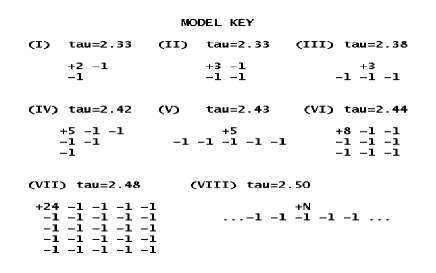
FIG. 1.: Toppling patterns and avalanche exponents for the models studied. The exponents are accurate to at least $\pm$ .01.

In our simulations we considered a variety of directed models with differing toppling vectors some of which are described in Fig.1. Model I was previously solved exactly by Dhar and Ramaswamy(DR)[5].

Abelian sandpile models(ASM) are conventionally driven by adding a grain of sand to a random site in a stable configuration. If this site becomes unstable then the appropriate toppling vector is subtracted from the new state perhaps inducing other sites to become unstable. On the next time step the lattice is reexamined for unstable sites which are then toppled. The number of time steps before no new unstable sites are found is said to be the avalanche’s lifetime. The total number of toppled sites is called the avalanche’s size or mass. Once the system relaxes, another grain is randomly added to the new stable state. DR showed that once an ASM is driven into the stationary state by this method, all reccurent configurations occur with equal probability. So in theory at least, one could get the same statistics by adding sand to random members of the recurrent set. Typically this is no small task since for the general ASM the recurrent set is remarkably complex. However, there is an infinite set of relaxation rules falling under the directed model classification which posess trivial recurrent sets. It can be shown that if there exists an orthogonal transformation which leaves the toppling matrix, $\Delta_{ij}=[\vec{T}_{j}]_{i}$, triangular, the recurrent set will consist of all possible stable configurations. [7, 6]. All of the models we simulated posess this trivial stationary state.

Since an avalanche may be seeded at a site near a boundary, even small avalanches may be effected by the finite system size. However, given the nature of these directed model’s stationary states and the fact that all sites in the lattice are equivalent to the extent that the system is infinite, one may reduce edge effects by introducing sand at a fixed site a maximum distance from the boundaries in randomly constructed stable states. Mass data from the simulations was obtained by seeding avalanches at the top left lattice site for models I, II, IV, VI, and VII and in the middle of the top row for for models III, V, and VIII. This mass was histogrammed, logarithmically binned and fitted to distributions of the form $\mathcal{P}$$(s)$$\propto$ $s^{1-\tau}$ where $\mathcal{P}$$(s)$ is the probability of the occurence of an avalanche with $s$ toppled sites. As can be seen from the plots in Fig.2, in which model V was used, the deviation from power law behavior in the simulation where sand is dropped on a fixed site is much more marked than in the simulation with a random drop site. This eliminates much of the guess work in finding a suitable endpoint for the linefitting routine. Notice also that the region of power law behavior in the run with the fixed drop site is at least as large as that of the run with the random drops even though it has a considerably smaller lattice.

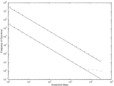
FIG. 2.: The lower curve is calculated for model V by seeding at a fixed site and using a random background on a 500x1000 lattice, the upper curve by seeding at random locations on a 3000x7000 lattice. The exponent in this case is 2.43

For the different models we found a range of values for $\tau$ from 2.33 to 2.50. The data is summarized in Fig.3, and exponents are given in Fig. 1. Although a general trend of increasing $\tau$ with increasing $h_{c}$ was observed, it was also found that $\tau$ varied with changes in ${\mathcal{N}}_{i}$ for a fixed $h_{c}$.

In model II, avalanches occur with the same distribution as the exactly solvable model I. This is understandable by observing that neither model allows untoppled sites, or ”holes”, in the interiors of their avalanche’s constant time surfaces. It was this fact which was essential to DR’s mapping of the evolution of the perimeter of an avalanche onto the problem of annhilating random walkers. Model II, may be similarly mapped, although with a different distribution over the walker’s step sizes. The difference in possible step sizes affects the variance of the walk, but not the exponent for the time of intersection. The distributions for the lifespans of these walkers are then the same as that of the avalanches and are identical for both models. However, it is possible for another choice of ${\mathcal{N}}_{i}$ with $h_{c}=3$ to produce avalanches with holes and complicated perimeters not suitable for description by random walkers. Model III is one such case as can be seen from Fig.4, and indeed, a different value for $\tau$(see Fig.1.) is obtained from its simulation. In general, as $h_{c}$ increases and the toppling vectors change, different patterns of holes are allowed, and different exponents result. This suggests that any classification of directed models must include a description of hole formation.

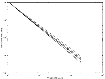
FIG. 3.: Data for the models described in Fig 1. The smallest exponent is from Models I and II, the largest from a simulation of an approximation to the infinite range model described in the text with an N of 100 and $\nu$ of 2. The data has been normalized to make the frequency in the first bin the same for all datasets.

An analytically tractable model has been devised to explore the limiting case of infinite $h_{c}$. The model lives on a $2d$ $MxN$ lattice with $h_{c}=N+\nu-1$ where $\nu$ is some positive integer. A site becomes unstable if it possesses $N+\nu$ or more grains. The $i_{th}$ unstable site is relaxed by subtracting the toppling vector $\vec{T}_{i}$. The components of $\vec{T}_{i}$ are given below.

$$[\vec{T}_{i}]_{s}=\left\{\begin{array}[]{ll}N+\nu&\mbox{if $s=i$}\\ -1&\mbox{for $s\in$ the next row}\\ 0&\mbox{$s\not=i$ and $s\not\in$ the next row}\par\end{array}\right.$$ (2)

In words, if a site becomes unstable and topples, $N+\nu$ grains of its sand are removed and one grain is added to every site in the next row so that $\nu$ grains are lost with each topple. Labeling the lattice sites by the convention which calls the upper left lattice site one and numbers sites across the first row to $N$ beginning the next row with $N+1$ and so on, one finds the toppling matrix to be lower triangular. As stated earlier this implies that the critical state consists of all stable configurations placing this model in the same category as the rest of the models considered in this treatment.

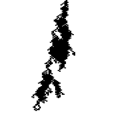
FIG. 4.: This is an avalanche for model III chosen to illustrate the hole formation. Note the presence of untoppled sites(white) within the boundaries of the avalanche

Note that with this model and for an avalanche beginning with a single unstable site, the constant time surfaces and therefore toppling activity are restricted to a single row. This allows the row by row evolution of an avalanches’ mass to be described by the properties of a stationary Markov chain with the row number serving also as the time parameter.

Let ${\mathcal{S}}_{n}$ be the random variable associated with the number of sites which topple on the $n^{th}$ row.Since a sites height in the stationary state can take values from $0$ to $N+\nu-1$ with equal probability, the conditional probability that a single stable site has $z$ grains and topples given that $i$ topple on the previous row is

$${\mathcal{P}}[{\mathcal{S}}_{n+1}={\hbox{1}}|{\mathcal{S}}_{n}=i]=\mathcal{P}[{\hbox{z}}\geq N+\nu-{\hbox{i}}]=\frac{i}{N+\nu}$$ (3)

.

The probabilities of different sites toppling on the same row are independent so the transition probabilty, $p_{ij}$, of $j$ sites toppling given that $i$ toppled on the previous row can be written as,

$${\mathcal{P}}[{\mathcal{S}}_{n+1}=j|{\mathcal{S}}_{n}=i]=\left(\begin{array}[]{c}N\\ j\end{array}\right){\left(\frac{i}{N+\nu}\right)}^{j}{\left(\frac{N+\nu-i}{N+\nu}\right)}^{N-j}$$ (4)

It is well known that a binomial distribution of this form approaches a Poisson distribution in the limit of large $N$ so that the above transition probability may be reexpressed as,

$$\lim_{N\rightarrow\infty}{p}_{ij}=\frac{i^{j}}{j!}e^{-i}$$ (5)

.

Letting $\mathcal{T}$ be the random variable associated with the avalanche lifetime, (or equivalently the number of rows which have at least one toppling event), it is clear that

$${P}[{\mathcal{T}}\leq n]={P}[{\mathcal{S}}_{n+1}=0]$$ (6)

and so

$${P}[{\mathcal{T}}\leq n]={P}[{\mathcal{S}}_{1}=0]+{P}[{\mathcal{S}}_{n+1}=0|{\mathcal{S}}_{1}=1]{P}[{\mathcal{S}}_{1}=1]$$ (7)

for avalanches begun by adding a single grain to the first row. ${P}[{\mathcal{S}}_{1}=0]$ and ${P}[{\mathcal{S}}_{1}=1]$ are constants for a fixed system size and ${P}[{\mathcal{S}}_{n+1}=0|{\mathcal{S}}_{1}=1]$ can be expanded in terms of the transition probabilities as,

$${P}[{\mathcal{S}}_{n+1}=0|{\mathcal{S}}_{1}=1]=\sum_{s_{n}=0}^{N}\sum_{s_{n-1}=0}^{N}\ldots\sum_{s_{2}=0}^{N}p_{s_{n}0}p_{s_{n-1}s_{n}}\ldots p_{1s_{2}}$$ (8)

. Carrying out the above sums for different $n$’s leads to the following sequence of conditional probabilities.

$$\begin{array}[]{l}{P}[{\mathcal{S}}_{1}=0|{\mathcal{S}}_{1}=1]=0\\ {P}[{\mathcal{S}}_{2}=0|{\mathcal{S}}_{1}=1]=e^{-1}\\ {P}[{\mathcal{S}}_{3}=0|{\mathcal{S}}_{1}=1]=e^{{P}[{\mathcal{S}}_{2}=0|{\mathcal{S}}_{1}=1]-1}\\ \vdots\\ {P}[{\mathcal{S}}_{n+1}=0|{\mathcal{S}}_{1}=1]=e^{{P}[{\mathcal{S}}_{n}=0|{\mathcal{S}}_{1}=1]-1}\end{array}$$ (9)

Expanding ${P}[{\mathcal{S}}_{n}=0|{\mathcal{S}}_{1}=1]$ in powers of $\frac{1}{n}$ and using the above recursion to find the coefficients, one finds that to first order,

$${P}[{\mathcal{S}}_{n}=0|{\mathcal{S}}_{1}=1]=1-\frac{2}{n}$$ (10)

. So that for long lived avalanches in large systems, we find that the probability of an avalanche lasting longer than $n$ time steps is

$${P}[{\mathcal{T}}>n]\simeq\frac{A}{n^{\alpha}}$$ (11)

where $A=2{P}[{\mathcal{S}}_{1}=1]$ and $\alpha=1$. The average flux of grains in and out of a row in the steady state must be constant. This implies that the probability of the mass of an avalanche being greater than $m$ is proportional to $m^{2-\tau}$ where $\tau$ is given by the relationship $\tau=2+\alpha/(1+\alpha)$ [5]. This value of $2.5$ for $\tau$ matches the value obtained by numerical simulation to within $\pm.01$ for $N=100$ and $\nu$=2.

From the point of view of the analogy with equilibrium critical systems, the continuous variation of the avalanche exponent with the range and details of the interaction is not understandable. There are of course equilibrium models with varying exponents, such as the Ashkin-Teller model, but we see no connection of the SOC models we have considered with these models. Varying exponents have also been obtained in dissipative SOC models, such as the one introduced by Olami, Feder, and Christensen[8], but in these models, the dissipation, which effectively links every site to the boundary, is a long ranged interaction, and so the variation of exponents is at least not in contradiction with the intuition gained from equilibrium systems.[9]

However, in our case, the models intermediate between the DR model and the mean field model we have introduced are all short ranged in the usual sense of equilibrium critical phenomena. They should all have the same critical exponents, which is Ben-Hur and Biham’s conjecture, and they do not. We do not think that the natural point of view from this perspective, that we are just not yet in the critical region for the data we have shown, and they will all eventually cross over to a common exponent of 2.33, is tenable. By using the fact that the recurrent set is the stable cube for our models, we eliminate the problem of long transients or uncertainty in the exponent due to edge effects. For model three, the system size used is about 100 times the interaction range, which is the only scale in the problem. If there was going to be a cross-over, we should have seen it. We conclude that there is no universality in those 2-d directed models whose avalanches from recurrent states contain holes. The extent to which the breakdown of universality extends to other SOC models remains to be seen[10].

Acknowledgement

We thank Maya Paczuski for her encouragement and many useful conversations. This work was supported by the Texas Center for Superconductivity through a grant from the state of Texas.

REFERENCES

- [1] Stefan Boettcher and Maya Paczuski, Phys. Rev. Letts. 77,111 (1996)
- [2] R. Burridge and L. Knopoff, Bull. Seismol. Soc. Am 57, 341 (1967)
- [3] Dinko Cule and Terence Hwa, Phys. Rev. B 57, 8235 1998
- [4] A. Ben-Hur and O. Biham, Phys. Rev. E, 53, R1317 (1996)
- [5] Deepak Dhar and Ramakrishna Ramaswamy, Phys. Rev. Letts. 63, 1659 (1989)
- [6] D. Dhar, Phys. Rev. Letts. 64, 1613 (1990)
- [7] thesis, Rick Tully, (to be published)
- [8] Z. Olami, H.J.S. Feder and K. Christensen, Phys. Rev. Letts 68, 1244, (1992);K. Christensen and Z. Olami, Phs. Rev. A 46, 1829 (1992)
- [9] An analysis of the reasons for the variation of the exponent in this case is given in A.Alan Middleton and Chao Tang, Phys. Rev. Letts. 74, 742 (1995)
- [10] A breakdown of universality in a non-abelian model has been reported in O.Biham,E.Milshtein and S. Solomon, cond-mat/9805206.