On the distribution of the total energy of a system of non-interacting fermions: random matrix and semiclassical estimates

Abstract

We consider a single particle spectrum as given by the eigenvalues of the Wigner-Dyson ensembles of random matrices, and fill consecutive single particle levels with $n$ fermions. Assuming that the fermions are non-interacting, we show that the distribution of the total energy is Gaussian and its variance grows as $n^{2}\log n$ in the large-$n$ limit. Next to leading order corrections are also computed. Some related quantities are discussed, in particular the nearest neighbor spacing autocorrelation function. Canonical and grand canonical approaches are considered and compared in detail. A semiclassical formula describing, as a function of $n$, a non-universal behavior of the variance of the total energy starting at a critical number of particles is also obtained. It is illustrated with the particular case of single particle energies given by the imaginary part of the zeros of the Riemann zeta function on the critical line.

^aDivision de Physique Théorique, Institut de Physique Nucléaire.
91406, Orsay Cedex, France. ^bDepartamento de Física, Facultad de Ciencias Exactas y Naturales,
Universidad de Buenos Aires. Ciudad Universitaria, 1428 Buenos Aires, Argentina.

Submitted for publication to Physica D – April 27, 1998.

Dedicated to our friend Boris Chirikov,
. with respect and admiration.              

I Introduction

Consider a system of $n$ interacting fermions. The ground state total energy may often be well approximated by macroscopic methods, a prototype of these being the Thomas-Fermi approximation. Aside from the well-known expansion containing the volume energy, surface energy, etc, these methods can be further improved by the inclusion of additional systematic quantum effects, like for example shell effects related to some symmetries of the system (see for instance [1]). Once all these contributions have been taken into account, one would like to have some estimate of the remaining “irreducible” discrepancies between the calculated and measured total energies due to non-systematic effects. These discrepancies may be viewed as fluctuations observable as some parameters of the system are varied, like for example the total number of particles or any other relevant external parameter.

On the other hand, it has been established that statistical properties of systems whose classical analog is chaotic are well described by eigenvalues of ensembles of random matrices (see for instance [3]). It seems therefore reasonable to suggest that an extreme estimate of the above mentioned fluctuations may consist of modeling the single particle spectrum by the spectrum of a random matrix of the Wigner-Dyson type. This may be a crude approximation because the statistical properties of the low-lying energy levels of the single particle sequence may not be well described by a random matrix approach. Another shortcoming of such a model is connected to the fact that, for simplicity, we fix to a constant the average density of single particle states, and ignore its variations with energy. In its simplest version, the model may apply either when only properties around the Fermi level are considered or when particles are enclosed in a $2$-dimensional box. However, inclusion of a variation (increase) of the density of single particle energies can be taken care of. This model may also be relevant in studying the energy distribution of systems of interacting fermions trapped in a chaotic enclosure, like for example the variations of the total energy of $n$ electrons contained in a quantum dot as the shape of the dot is varied by some external potential or the variation produced when varying a magnetic field.

To be specific, consider an ordered sequence of energy levels $x_{0}<x_{1}<\ldots<x_{i}<\ldots$. Let $s_{1},\ s_{2},\ s_{3},\ldots$ be the distances between consecutive eigenvalues,

$$s_{i}=x_{i}-x_{i-1}\ .$$

We assume that the sequence is stationary and we set the mean spacing $D$ to one. We are interested in the statistical properties of the “ground state” energy $X_{t}$ of a system of $n$ non-interacting fermions resulting from adding the “single particle” energies $x_{i}$ of the $i=1,2,\ldots,n$ occupied states

$$X_{t}(n)=\sum_{i=1}^{n}(x_{i}-x_{0})=\sum_{i=1}^{n}(n-i+1)\;s_{i}\;,$$ (1)

where $x_{0}$ has been taken as the energy origin. Consider now an ensemble of single particle spectra which for the moment we let unspecified. We expect under very general conditions the probability distribution of $X_{t}$ to be Gaussian in the large $n$ limit. This, by the central limit theorem, is obviously true for a set of uncorrelated levels. For (correlated) eigenvalues of Gaussian ensembles of random matrices this has also shown to be true, in fact in a more general context [4]. As a numerical illustration, Fig. 1 displays the probability distribution of $X_{t}$ for $n=300$ computed for a Gaussian orthogonal ensemble of random matrices. Our purpose is to derive expressions for the average and the variance of $X_{t}$, thereby specifying completely the “ground-state” energy distribution.

The first physical situation we consider is when the number $n$ of particles is fixed. This case, which we call “canonical” by analogy to conventional statistical mechanics, is treated in section II. From the mathematical point of view it is related to the autocorrelation function of consecutive spacings, a poorly known quantity which is not a two-point measure. Another possibility is to consider the typical fluctuations of the total energy of the occupied levels contained in an energy interval of given length. In this case the number $n$ of levels fluctuates from sample to sample around its mean value. This alternative “grand canonical” problem will be treated and compared to the canonical one in section III. The grand canonical case has the advantage of being expressible in terms of the spectral two-point correlation function. As expected we find that both approaches give the same asymptotic increase of the variance of the total energy (proportional to $n^{2}\log n$ in the large-$n$ limit).

The results of sections II and III correspond to the “universal regime” as given by random matrix theory. In section IV we use standard semiclassical techniques to show that generically for ballistic – as opposed to diffusive [5] – systems there is a saturation effect, namely a crossover from the $n^{2}\log n$ to a $n^{2}$ growth of the variance of the total energy as a function of $n$. This new regime holds when the number of particles is larger than a system-dependent critical value and is accompanied by non-universal oscillations around the mean growth for which we give an explicit expression. To illustrate this point with a particular example, we have considered the unphysical but interesting in its own and explicitly computable case where the single particle energies are given by the imaginary part of the zeros of the Riemann zeta function on the critical line. Section V summarizes the results and gives some perspectives.

II Canonical Variance

Statistical averages over the ensemble are denoted by the symbol $\langle.\rangle$. The mean value $\langle X_{t}\rangle$ is

$$\langle X_{t}\rangle=\sum_{i=1}^{n}(n-i+1)\langle s_{i}\rangle=\sum_{i=1}^{n}(n-i+1)=\frac{n(n+1)}{2}\;,$$ (2)

where the mean level spacing has been set equal to one.

Let us now consider the variance of $X_{t}$ defined, from Eq.(1), by

$$\Delta^{2}(n) \equiv \langle X_{t}^{2}\rangle-\langle X_{t}\rangle^{2}=\sum_{i,j=1}^{n}(n-i+1)(n-j+1)\;\langle s_{i}\;s_{j}\rangle-\frac{1}{4}n^{2}\;(n+1)^{2}$$ (3)

$$= \;\sum_{i=1}^{n}(n-i+1)^{2}\langle s_{i}^{2}\rangle+\sum_{i\neq j=1}^{n}(n-i+1)(n-j+1)\langle s_{i}s_{j}\rangle-\frac{1}{4}n^{2}\;(n+1)^{2}\;.$$ (4)

The main quantity of interest in this expression is the autocorrelation function $I(k)$ of spacings of consecutive levels,

$$I(k)\equiv\langle s_{i}s_{i+k}\rangle\;\;\;\;\;\;\;\;\;\;\;k=1,..,n-1\;.$$

The stationarity of the spectrum implies that $I(k)$ depends only on the relative index $k$ and that $\langle s_{i}^{2}\rangle=\langle s^{2}\rangle$, for all $i$. Performing the sums over the index $i$

$$\Delta^{2}(n)=\frac{n(n+1)(2n+1)}{6}\langle s^{2}\rangle-\frac{1}{4}n^{2}\;(n+1)^{2}+\frac{1}{3}\sum_{j=1}^{n-1}F(n,j)\;I(j),\;\;\;\;\;n\geq 2\;,$$ (5)

where

$$F(n,j)\equiv j^{3}-(3n^{2}+3n+1)j+n\ (n+1)\ (2n+1)\;.$$

For $n=1$ the variance takes the value $\Delta^{2}(1)=\ \langle s^{2}\rangle\ -1$. All the non-trivial information is contained in the autocorrelation of spacings; a detailed study of this function will be made in the next subsection. The extreme case of a uniform uncorrelated sequence of levels is particularly simple since $I(j)=1$ for all $j$, and it follows from Eq.(5) that

$$\Delta^{2}_{u}=(\langle s^{2}\rangle_{u}\ -1)\left(\frac{n^{3}}{3}+\frac{n^{2}}{2}+\frac{n}{6}\right)\;.$$ (6)

When the nearest neighbor spacing distribution of the uncorrelated sequence is $P(s)=\exp(-s)$ then ${\langle s^{2}\rangle}_{u}$ in Eq.(6) is equal to $2$.

A The autocorrelation function of spacings $I(j)$

For Gaussian ensembles (GE) of random matrices, the quantities entering Eq.(5) can be expressed as

$$\langle s^{2}\rangle = 2\;\int_{0}^{\infty}E(0,s)\;ds\;,$$ (7)

$$I(j) = \;\int_{0}^{\infty}E(j,s)\;ds,\;\;\;\;\;\;\;\;\;j\geq 1,$$ (8)

where $E(j,s)$ is the probability that a randomly chosen interval of length $s$ contains exactly $j$ eigenvalues [6]. The functions $E(j,s)$ can be written in terms of an infinite product of the eigenvalues of an integral equation involving spheroidal functions and only numerical tables of these functions for low values of $j$ and a limited range of $s$ exist. Therefore the integrals in (8) cannot be computed analytically and explicit expressions for the $I(j)$ are not available. Some numerical estimates of the integrals (8), to be used in what follows, are [6]

$${\langle s^{2}\rangle}=\left\{\begin{array}[]{ll}1.286,&\;\;\;\;\;\;\;\;\;\;\mbox{$\beta=1$}\\ 1.180,&\;\;\;\;\;\;\;\;\;\;\mbox{$\beta=2$}\\ 1.105,&\;\;\;\;\;\;\;\;\;\;\mbox{$\beta=4$}\end{array}\right.$$ (9)

where $\beta\;=1,2$ and $4$ denote the three types of GE, orthogonal (GOE), unitary (GUE) and symplectic (GSE) respectively. Numerical estimates of $I(j)$ exist for low values of $j$. For instance, for $j=1$ [6]

$$I(1)=\left\{\begin{array}[]{ll}0.922,&\;\;\;\;\;\;\;\;\;\mbox{$\beta=1$}\\ 0.944,&\;\;\;\;\;\;\;\;\;\mbox{$\beta=2$}\\ 0.964,&\;\;\;\;\;\;\;\;\;\mbox{$\beta=4$.}\end{array}\right.$$ (10)

For our purpose the functions $I(j)$ for arbitrary $j$ are needed and the following ansatz

$$I(j)=\;1\,-\eta/j^{2}\,-\lambda/j^{4}\,-\alpha/j^{6}$$ (11)

will be made. The constants in Eq.(11) are, in principle, dependent on the symmetry class of the GE considered ($\beta=1$, $2$, $4$). Eq.(11) is one of the basic equations of this paper. The simple functional dependence on $j$ is consistent with the requirement that two sufficiently far apart consecutive spacings should be uncorrelated. Moreover, general considerations suggest that odd powers of $j$ may be excluded. As we will now show, the three parameters entering Eq.(11) may be uniquely determined by requiring the correct asymptotic behavior of the fluctuations in the length of an interval containing a fixed number of levels.

Consider for that purpose the statistical fluctuations in the length $S$ of a spacing made of $n$ consecutive nearest-neighbor spacings, $S=\displaystyle\sum_{i=1}^{n}s_{i}\;$. The spacing variance $\sigma^{2}$ of $S$ can be expressed in terms of the $I(j)$ in the following manner

$$\sigma^{2}(n)\equiv\ \langle S^{2}\rangle-{\langle S\rangle}^{2}=\;n\left(\langle s^{2}\rangle-n\right)+2\;\sum_{j=1}^{n-1}(n-j)\;I(j),\;\;\;\;\;\;n\geq 2\;,$$ (12)

while $\sigma^{2}(1)\equiv\langle s^{2}\rangle-1$. We use a non-conventional but more natural notation, namely $\sigma^{2}(n)$ denotes the variance of the distribution of the sum of $n$ consecutive nearest neighbor spacings ($n=1,2,\ldots$). The conventional notation being $\sigma^{2}(n-1)$, $n=1,2,\ldots$.

Replacing the ansatz (11) in (12) we get

$$\sigma^{2}(n) = \;\left(\langle s^{2}\rangle-1\right)\ n\ +2\ \eta\ \left[\Psi(n)+\gamma\right]+2\ \eta\ n\ \left[\Psi^{(1)}(n)-\zeta(2)\right]+\lambda\ \left[\Psi^{(2)}(n)+2\;\zeta(3)\right]$$ (15)

$$+\ (n\ \lambda/3)\left[\Psi^{(3)}(n)-6\ \zeta(4)\right]+(\alpha/12)\left[\Psi^{(4)}(n)+24\ \zeta(5)\right]$$

$$+\ (n\ \alpha/60)\left[\Psi^{(5)}(n)-120\ \zeta(6)\right]\ ,$$

where $\gamma$ is the Euler constant, $\Psi(n)=-\gamma+\ \displaystyle\sum_{j=1}^{n-1}\frac{1}{j}$ is the DiGamma function and $\Psi^{(m)}(z)=\frac{d^{m}}{dz}\Psi(z)$ are the PolyGamma functions [7]. The large-$n$ behavior of $\sigma^{2}(n)$ follows from the asymptotics of the $\Psi^{(m)}$’s [7]. Only $\Psi$ and $\Psi^{(1)}$ will be needed, the other not contributing at the order we are working

$$\Psi(n) = \log n-\frac{1}{2n}-\frac{1}{12n^{2}}+{\cal}O(1/n{{}^{4}})\;,\,$$ (16)

$$\Psi^{(1)}(n) = \frac{1}{n}+\frac{1}{2n^{2}}+\frac{1}{6n^{3}}+{\cal O}(1/n^{5})\ .$$ (17)

Then

$$\sigma^{2}(n)=A\ n+2\ \eta\ \log n\ +B+\ {\cal O}(1/n^{2})\ ,$$ (18)

with

$$A \equiv {\langle s^{2}\rangle}-1-2\ \eta\ \zeta(2)\ -2\ \lambda\ \zeta(4)-2\ \alpha\ \zeta(6)\ ,$$ (19)

$$B \equiv 2\ (\gamma+1)\ \eta+2\ \lambda\ \zeta(3)+2\ \alpha\ \zeta(5)\ .$$ (20)

Would one have retained a $1/j$ term in the ansatz, the leading order term would have been of order $n\log n$.

A different quantity, closely related to the spacing variance $\sigma^{2}(n)$, is the number variance $\Sigma^{2}(L)$ defined as the variance of the number of levels contained in an interval of given length $L$ taken at random. This quantity is known analytically for the three Gaussian ensembles and has in the large-$L$ limit the asymptotic behavior [6]

$$\Sigma^{2}(L)=\frac{2}{\beta\pi^{2}}\log L+C+{\cal O}(1/L)\ ,$$ (21)

where

$$C=2/(\beta\pi^{2})\{\gamma+\log(2\pi)+1+\beta(\beta-2)\pi^{2}/8+[\log 2-7\pi^{2}/8]\delta_{\beta,4}\}\ .$$ (22)

Consider now more carefully the relation between the spacing and the number variances. The values that the number variance takes at integer values of its argument are, for large $n$, related to the spacing variance through [8]

$$\Sigma^{2}(L=n)-\sigma^{2}(n)=1/6\ .$$ (23)

This equation indicates that: (i) as expected from their definition, the leading order terms of both quantities coincide and, (ii) the next-to-leading order terms differ by a constant ($1/6$), irrespective of the symmetry class $\beta$.

Eq.(23) completely determines all the unknown coefficients in Eq.(11). In fact, consistency with Eq.(23) imposes the following conditions in Eq.(18)

$$\eta = \frac{1}{\beta\pi^{2}}\ ,$$ (24)

$$A = 0\ ,$$ (25)

$$C-B = 1/6\ .$$ (26)

The remaining free parameters $\lambda$ and $\alpha$ are adjusted to satisfy the second and third conditions

$$\lambda = \frac{\langle s^{2}\rangle-1-\ 2\ \eta\ \zeta(2)}{2\ \zeta(4)}-\frac{\zeta(6)}{\zeta(4)}\alpha\ ,$$ (27)

$$\alpha = \frac{\zeta(4)}{2[\zeta(3)\zeta(6)-\zeta(4)\zeta(5)]}\left\{2\ \eta\ (\gamma+1)-C+\frac{1}{6}+\ \frac{\zeta(3)}{\zeta(4)}\left[\langle s^{2}\rangle-1-2\ \eta\ \zeta(2)\right]\right\}\ .$$ (28)

Using Eq.(9) these two constants take the values $\lambda=0.02027,\ 0.03013,\ 0.00997$ and $\alpha=-0.04483,\ -0.02550,\ 4\times 10^{-5}$ for $\beta=1,2$ and $4$, respectively.

In order to test the accuracy of Eq.(11) we have computed numerically the autocorrelation function $I(j)$ for orthogonal as well as unitary random matrices. As can be seen from Fig. 2 the agreement between the ansatz and the numerical simulations for $\beta=2$ is very good. Because the overall agreement is of similar quality we do not show the analogous curve for GOE. As an additional quantitative test let us mention that when expression (11) is evaluated at $j=1$ it reproduces the values in Eq.(10) with a $1\times 10^{-3}$ error for any $\beta$. This is remarkable if one keeps in mind that only asymptotic information has been used when determining the parameters in the ansatz (11).

In a previous study of the autocorrelation function of the spacings Odlyzko [9] has quoted a conjecture proposed by Dyson: $I(j)\approx 1-\eta/j^{2}$ (see also chapter 16 in [6]). This ansatz coincides to lowest order with Eq.(11). Aside from considerations related to accuracy, let us emphasize that the inclusion of a term of higher order (like $1/j^{4}$ or $1/j^{6}$) in (11) is essential in order to obtain the correct asymptotic behavior for $\sigma^{2}(n)$ as well as, as we shall see later, for $\Delta^{2}(n)$. This is so because these higher order terms ensure the vanishing of the linear term in Eq.(18).

Eq.(11) is consistent with known relationships satisfied by the autocorrelation function. For example, the sum rule

$$2\sum_{j=1}^{\infty}\left[I(j)-1\right]+\sigma^{2}(1)=0$$

valid for GE of random matrices [10] is equivalent to the condition $A=0$ in Eq.(24) (i.e., the vanishing of the linear term of $\sigma^{2}(n)$ [11]).

B Variance of the total energy

We have now the necessary ingredients to compute the variance of the total energy. Replacing in Eq.(5) the ansatz (11) and using the definition of the DiGamma and PolyGamma functions it follows that

$$\Delta^{2}(n) = \frac{n^{2}}{2}\left(C-\frac{7\eta}{3}-\frac{1}{6}\right)+\frac{n}{2}\left(C-\frac{5\eta}{3}-\frac{1}{6}\right)+\frac{1}{6}\left(C-2\eta-2\ \gamma\ \lambda-2\ \alpha\ \zeta(3)-\frac{1}{6}\right)$$ (32)

$$+\Psi(n)\left[\eta\left(n^{2}+n+\frac{1}{3}\right)-\frac{\lambda}{3}\right]+\Psi^{(1)}(n)\ \eta\left(\frac{2n^{3}}{3}+n^{2}+\frac{n}{3}\right)$$

$$+\frac{1}{2}\Psi^{(2)}(n)\left[\lambda\left(n^{2}+n+\frac{1}{3}\right)-\frac{\alpha}{3}\right]+\frac{1}{6}\Psi^{(3)}(n)\ \lambda\left(\frac{2n^{3}}{3}+n^{2}+\frac{n}{3}\right)$$

$$+\frac{1}{24}\Psi^{(4)}(n)\ \alpha\left(n^{2}+n+\frac{1}{3}\right)+\frac{1}{120}\Psi^{(5)}(n)\ \alpha\left(\frac{2n^{3}}{3}+n^{2}+\frac{n}{3}\right)$$

for $n\geq 2$. Using again the asymptotic expressions (16) for $\Psi(n)$ and $\Psi^{(1)}(n)$, as well as those of $\Psi^{(2)}(n)$ and $\Psi^{(3)}(n)$ [7] we finally get

$$\Delta^{2}(n) = \eta\;n^{2}\log n+\frac{1}{2}\left(C-\eta-\frac{1}{6}\right)n^{2}+\eta\;n\log n+\frac{1}{2}\left(C-\frac{1}{6}\right)n$$ (34)

$$+\frac{1}{3}\;(\eta-\lambda)\log n\ +\frac{1}{6}\left[C+\frac{(\eta-1)}{6}-2\left(\gamma+\frac{5}{6}\right)\lambda-2\ \alpha\ \zeta(3)\right]+{\cal O}(1/n)\;.$$

Notice that, as it happened for $\sigma^{2}(n)$ with the terms of order $n\log n$ and $n$, the functional form of the ansatz (11) together with the method by which the parameters $\eta$, $\alpha$ and $\lambda$ have been determined insure the vanishing of the terms of order $n^{3}\log n$ and $n^{3}$ of the variance of the total energy. That the remaining leading order behavior $n^{2}\log n$ in Eq.(34) is correct is further confirmed by the fact that it coincides with the asymptotic result obtained from the linear statistic theory (see section III). This behavior is in contrast with the faster growth of order $n^{3}$ of an uncorrelated spectrum (cf Eq.(6)). The difference is of course due to the rigid nature of the GE spectra.

Fig. 3 shows for GOE the comparison of numerical results with Eq.(34) for the variance of the total energy as a function of $n$. The overall agreement is good (for $n\approx 50$ the relative error is less than $2\%$). The theoretical curve is sensitive to the precise value of $\langle s^{2}\rangle$ which enters in the definition of $\lambda$ and $\alpha$, and is known only up to the third digit (cf Eq.(9)). For comparison we have also plotted in Fig. 3 the leading-order term of $\Delta^{2}$, which clearly fails to reproduce accurately the numerical results in the interval of $n$ displayed (the error is of the order of 10% at $n\approx 50$).

In the previous analysis we have taken a single particle level ($x_{0}$ in (1)) as the reference energy. In some physical applications it may be more appropriate to measure energies with respect to an arbitrary origin, which will not coincide with a single particle level but rather will lie in a random position between two of them. As shown in Appendix A when this construction is adopted, namely filling $n$ successive levels located just above this origin, Eq.(2) giving the mean value of the energy is modified as follows $n(n+1)/2\rightarrow n^{2}/2$, whereas for the variance of the energy one has

$$\Delta^{2}(n)\rightarrow\Delta^{2}(n-1)+\frac{n^{2}}{2}\left(\frac{1}{2}-\frac{\langle s^{2}\rangle}{3}\right)+\frac{n}{2}\sigma^{2}(n)\ .$$ (35)

Notice that both sides of (35) have the same leading order, though different coefficients for higher order terms.

III Grand canonical Variance

Here we treat a slightly different problem with respect to the previous section. Instead of fixing the number of occupied levels, we consider an energy interval of given length $2L$ and compute the energy variance for the single particle energies $x_{1},\ldots,x_{n}$ contained in it (to follow conventional notation, in this section we will denote the length of the energy interval by $2L$, whereas in the previous section we were denoting it by $L$). The length $2L$ of the energy interval is now kept fixed but the number $n$ of levels contained in it may now vary from sample to sample. This is a particular example of a more general class of problems usually called “linear statistic” in random matrix theory [12], dealing with the distribution of a variable $W$ of the form

$$W=\sum_{i=1}^{n}f(x_{i})\;,$$ (36)

where $f$ is an arbitrary function. The variance of $W$ was given in [12]

$$V_{W}=\int\int_{-L/D}^{L/D}dx\ dy\left[\delta(x-y)-Y_{2}(x,y)\right]f(xD)f(yD)$$ (37)

or, alternatively, in the Fourier space

$$V_{W}=\frac{1}{D}\int_{-\infty}^{\infty}dk\left[1-b(Dk)\right]\varphi(k)\varphi(-k)\ .$$ (38)

Here $D$ is the mean level spacing (assumed to be constant; it will be set to one at the end), $Y_{2}$ the two-level cluster function, $b(k)=\int_{-\infty}^{\infty}Y_{2}(x)\;\exp[2i\pi kx]\;dx$ the form factor and $\varphi(k)$ the Fourier transform of $f(x)$

$$\varphi(k)=\int_{-L}^{L}f(x)\;\exp[-2i\pi kx]\;dx$$

($f(x)$ is assumed to be zero outside the interval $[-L,L]$).

To compute the number variance via Eq.(38), one must choose $f(x)=1$, as Dyson and Mehta did. For our purpose, namely to compute the variance of the total energy, $f(x)$ should be chosen as follows

$$f(x)=\left\{\begin{array}[]{ll}x+L&\mbox{$-L\leq x\leq L$}\\ 0&\mbox{$|x|>L$}\end{array}\right.$$ (39)

whose transform is

$$\varphi(k)=\frac{\rm i}{2\pi^{2}k^{2}}[2\pi Lk\cos(2\pi Lk)-\sin(2\pi Lk)]+\frac{L}{\pi k}\sin(2\pi Lk)\ .$$ (40)

In Eq.(39) we have chosen to measure the energy with respect to the lower (or equivalently upper) end of the energy interval considered. This, which is somewhat natural and analogous to Eq.(1), is by no means compulsory and the reference may be taken at any given point of the energy axis. The variance of the total energy depends on the location of the reference point, the minimum being obtained when it is at the center of the interval. A general relation connecting the variance at different reference points is given in Appendix B.

Let us now consider the case of a large (average) number $n$ of levels contained in the interval. Though we are using for notational simplicity the same symbol as in the canonical case, for grand canonical expressions $n$ will mean the expectation value $\langle n\rangle=2L/D$. Therefore, in contrast to the canonical case, it takes continuous values. Following Ref.[12], we split the integral in Eq.(38) in two parts

$$V_{E}=\frac{2}{D}\int_{0}^{\epsilon}\varphi(k)\varphi(-k)\ [1-b(Dk)]\ dk+\frac{2}{D}\int_{\epsilon}^{\infty}\varphi(k)\varphi(-k)\ [1-b(Dk)]\ dk$$ (41)

where we have used the parity of the integrand. The parameter $\epsilon$ is chosen such that $1/L\ll\epsilon\ll 1/D$. For $k<\epsilon$, $Dk$ is always much smaller than one and the form factor can be approximated by [6]

$$b(Dk)\approx 1-\frac{2D}{\beta}\ |k|$$

and the first term in the r.h.s. of Eq.(41) (denoted $V_{E}^{(a)}$) can be written

$$V_{E}^{(a)}=\frac{4L^{2}}{\beta\pi^{2}}\int_{0}^{2\pi L\epsilon}\ \left[\frac{1}{x}-\frac{2\cos x\sin x}{x^{2}}+\frac{\sin^{2}x}{x^{3}}\right]dx\ ,$$

which when integrated and taken in the limit $L\epsilon\gg 1$ gives

$$V_{E}^{(a)}\approx\frac{4L^{2}}{\beta\pi^{2}}\,[\log(2\pi L\epsilon)+\gamma+\log 2-1/2]\ .$$ (42)

On the other hand, for $k>\epsilon$ we have $kL\gg 1$ and the function $\varphi(k)$ shows rapid oscillations as compared to the variations of the form factor. We then replace the product $\varphi(k)\varphi(-k)$ in the second term of the r.h.s. of Eq.(41) (denoted $V_{E}^{(b)}$) by its average value over $k$

$$\langle\varphi(k)\varphi(-k)\rangle_{k}=\frac{L^{2}}{\pi^{2}k^{2}}+\frac{1}{8\pi^{4}k^{4}}$$

and then

$$V_{E}^{(b)}\approx-\frac{2L^{2}}{\pi^{2}}\int_{D\epsilon}^{\infty}\frac{[b(x)-1]}{x^{2}}\ dx-\frac{D^{2}}{4\pi^{4}}\int_{D\epsilon}^{\infty}\frac{[b(x)-1]}{x^{4}}\ dx\ .$$

The second integral in the latter equation is of order $1/(\epsilon L)^{2}$ with respect to the first one and therefore can be neglected. Evaluating the first integral we get

$$V_{E}^{(b)}\approx\frac{-4L^{2}}{\beta\pi^{2}}\left[\log(D\epsilon)-1\right]+(\beta-2)\frac{L^{2}}{2}\ .$$ (43)

Collecting the two terms we obtain the final expression for the variance which we express in terms of the average number $n$ of levels contained in the interval and the constant $C$ (cf (22)) (we put moreover $D=1$)

$$V_{E}(n)\approx\eta\ n^{2}\log n+\frac{1}{2}\left(C-\eta\right)n^{2}\ .$$ (44)

Let us now compare grand canonical and canonical results. When the sequence considered is large ($n\gg 1$), we expect the energy variance computed for a fixed number $n$ of occupied levels ($\Delta^{2}$, canonical) to be equal to the energy variance when the fixed length of the energy interval contains on the average $n$ levels ($V_{E}$, grand canonical). The comparison of Eqs.(44) and (34) shows that indeed to leading order $V_{E}=\Delta^{2}$ (the same leading order behavior has been obtained in Ref.[13] for the particular case of GOE employing Dyson Brownian motion). However the correction terms are different. It is interesting to note that the next to leading order corrections differ, as in Eq.(23) for the number and spacing variances, by a constant independent of $\beta$

$$\lim_{n\rightarrow\infty}\frac{V_{E}(n)-\Delta^{2}(n)}{n^{2}}=\frac{1}{12}\ ,$$ (45)

which follows from Eqs.(34) and (44).

To conclude this subsection let us point out that exact expressions for the energy variance can be computed in the grand canonical approach for any value of $n$ without assuming that it is large. For example for the unitary case $(\beta=2)$ from the definition Eq.(38), using Eq.(40) and the fact that

$$b(k)=\left\{\begin{array}[]{ll}1-\;\mid k\mid&\mbox{$\mid k\mid\leq 1$}\\ 0&\mbox{$\mid k\mid>1$}\end{array}\right.$$ (46)

it follows that

$$V_{E}(n)=\frac{n^{2}}{2\pi^{2}}\left[\begin{array}[]{l}\displaystyle\log n-{\rm Ci}(2\pi n)-\frac{4\pi n}{3}{\rm Si}(2\pi n)+\frac{\sin(2\pi n)}{6\pi n}+\left(\frac{1}{12\pi^{2}n^{2}}-\frac{2}{3}\right)\cos(2\pi n)\end{array}\right.$$

$$\left.\begin{array}[]{l}-\displaystyle\frac{1}{12\pi^{2}n^{2}}+\frac{2\pi^{2}n}{3}+\gamma+\log(2\pi)+\frac{1}{2}\end{array}\right]\ ,\;\;\;\;\;\;\;\;\beta=2\ ,$$ (47)

where ${\rm Ci}(x)$ and ${\rm Si}(x)$ are the CosIntegral and SinIntegral functions[7], respectively. $V_{E}(n)$ grows like $n^{3}$ for $n\rightarrow 0$ (remember that here $n$ is a continuous variable) and then switches to the $n^{2}\log n$ behavior for larger values of $n$.

IV Semiclassical treatment: Non-universalities

A Chaotic Systems

The strength and vitality of random matrix theories rely heavily on the universality of some of its predictions. As a counterpart it is poorly adapted to capture some system-specific features. However special tools have been developed for that purpose to study systems whose classical analog is chaotic. Indeed, one of the important achievements of semiclassical theories has been to determine the limits of validity of the universal regime as described by random matrix theories by including system-dependent corrections [14]. Our purpose now is to adapt these methods, which have been developed for the form factor and are thus applicable to the grand canonical case, to the study of the variance of the total energy.

Our starting point will be Eq.(38) written in a slightly different form

$$V_{W}=\frac{2}{D^{2}}\int_{0}^{\infty}d\tau K(\tau)\varphi(\tau/D)\varphi(-\tau/D)\ .$$ (48)

Here $K(\tau)=1-b(\tau)$ and we have used the parity of the integrand. For simplicity we restrict in the following to systems having no time reversal symmetry ($\beta=2$). The results can be easily generalized to the other symmetry classes.

In the previous section we computed the universal behavior of the variance of the total energy by inserting in (48) the random matrix spectral form factor (cf Eq.(46) for the unitary ensemble). It is possible however to give a more accurate description of the form factor based on semiclassical approximations. For systems having a classical analog the key ingredient is a formula expressing the spectral density $\rho(E)=\displaystyle\sum_{j}\delta(E-E_{j})$ as a sum over the classical periodic orbits

$$\rho(E)\approx\langle\rho(E)\rangle_{E}+\frac{1}{\pi\hbar}\sum_{p}\sum_{r=1}^{\infty}A_{p,r}\cos\left(rS_{p}/\hbar\right)\ .$$ (49)

Here $\langle\rho(E)\rangle_{E}=1/D$ is the spectral average density of states, $A_{p,r}=T_{p}/\sqrt{|\det(M_{p}^{r}-1)|}$ is an amplitude that depends on the period $T_{p}$ and the stability matrix $M_{p}$ of the primitive orbit $p$, $r$ are the repetitions and $S_{p}$ is the action [15]. We restrict our considerations to chaotic systems for which periodic orbits are isolated and unstable.

Using Eq.(49) for the density of states Berry [14] proposed the following form for $K(\tau)$ for chaotic systems

$$K(\tau)=\left\{\begin{array}[]{ll}(D/h)\displaystyle\sum_{p,r}A_{p,r}^{2}\ \delta(T-rT_{p})&\mbox{$\tau<\tau^{*}$}\\ \tau&\mbox{$\tau^{*}<\tau\leq 1$}\\ 1&\mbox{$\tau>1$}\ ,\end{array}\right.$$ (50)

where $h$ is Planck’s constant and $\tau=TD/h$ is the (rescaled) time measured in units of the Heisenberg time. The main physical ingredient entering this formula is a classical sum rule due to Hannay and Ozorio de Almeida [16] which takes into account the exponential proliferation of long periodic orbits as well as their ergodicity. As a consequence of this as well as other semiclassical considerations the form factor for times $\tau$ larger than a certain critical time $\tau^{*}$ becomes “universal” (i.e., coincides with random matrix theory). The situation is different for short periodic orbits which do not display this universality and whose contributions, explicitly written down in Eq.(50), produce system-dependent deviations from random matrix theory for $\tau<\tau^{*}$. Usually the parameter $\tau^{*}$ is chosen in order to satisfy $\tau_{\rm min}\ll\tau^{*}\ll 1$, where $\tau_{\rm min}=T_{\rm min}D/h$ is the rescaled period of the shortest periodic orbit.

The contribution of short periodic orbits to the variance of the total energy is obtained by replacing $K(\tau)$ for $\tau<\tau^{*}$ in Eq.(48), with the result

$$\frac{2}{h^{2}}\sum_{p,r}{\hat{A}}_{p,r}\ \varphi(r\tau_{p}/D)\ \varphi(-r\tau_{p}/D)\ .$$ (51)

Here ${\hat{A}}_{p,r}=h^{2}\tau_{p}^{2}/(D^{2}\sqrt{|\det(M_{p}^{r}-1)|})$ is the usual amplitude $A_{p,r}$ written in terms of the rescaled time $\tau_{p}$.

For times $\tau>\tau^{*}$ we can repeat the same steps as in the previous section (the form factor coincides with GUE), with the important difference however that now there is a cutoff in the integral (48) at $\tau=\tau^{*}$. The variance of the total energy may now be written in the following form

$$V_{E}(n)=V_{E}^{(1)}(n)+V_{E}^{(2)}(n)+V_{E}^{(3)}(n)\ ,$$ (52)

where $V_{E}^{(1)}$ is the GUE result (47) and

$$V_{E}^{(2)}(n) = -\frac{D^{2}n^{2}}{2\pi^{2}}\left[\log(n\tau^{*})+\frac{\cos(2\pi n\tau^{*})}{(2\pi n\tau^{*})^{2}}+\frac{\sin(2\pi n\tau^{*})}{2\pi n\tau^{*}}-{\rm Ci}(2\pi n\tau^{*})-\frac{1}{(2\pi n\tau^{*})^{2}}\right.$$ (54)

$$\left.\;\;\;\;\;\;\;\;\;\;\;\;\;+\log(2\pi)+\gamma-\frac{1}{2}\right]\ ,$$

$$V_{E}^{(3)}(n) = \frac{D^{4}n^{2}}{2\pi^{2}h^{2}}\sum_{r\tau_{p}<\tau^{*}}\frac{{\hat{A}}_{p,r}^{2}}{r^{2}\tau_{p}^{2}}\left\{\left[\cos(\pi nr\tau_{p})-\frac{\sin(\pi nr\tau_{p})}{\pi nr\tau_{p}}\right]^{2}+\sin^{2}(\pi nr\tau_{p})\right\}\ .$$ (55)

$V_{E}^{(2)}$ is the contribution to the variance due to the lower limit at $\tau=\tau^{*}$ in the integral (48). Aside from the system-dependent parameter $\tau^{*}$, its functional form is general. $V_{E}^{(3)}$ is obtained from (51) using the explicit form (40) of the Fourier transform $\varphi$ and contains detailed system-specific information.

The energy variance as a function of the number of particles exhibits now two different regimes. For $n\ll 1/\tau^{*}$, $V_{E}^{(2)}$ and $V_{E}^{(3)}$ are of order $(n\tau^{*})^{2}$ and can therefore be neglected. The energy variance is then given by the random matrix expression. For $n\approx 1/\tau^{*}$ these two terms can no longer be neglected and there is a crossover to a different regime, not described by random matrix theory. This is clearly seen for $n\gg 1/\tau^{*}$ when there is an almost perfect cancellation between $V_{E}^{(1)}$ and $V_{E}^{(2)}$, leading to

$$V_{E}(n)\approx\frac{D^{2}n^{2}}{2\pi^{2}}\left[1-\log\tau^{*}+{\cal O}(1/n\tau^{*})^{2}\right]+V_{E}^{(3)}(n)\;\;\;\;\;\;\;\;\;\;\;\;\;\;n\gg 1/\tau^{*}\ .$$ (56)

From Eq.(54) for $V_{E}^{(3)}$ we then see that now the variance instead of growing as $n^{2}\log n$ like in random matrix theory, saturates and increases as $\kappa\ n^{2}$. The prefactor $\kappa$ is not constant but shows non-universal oscillations as a function of $n$ described by the short-periodic-orbit contributions. In order to determine its average value over $n$ we replace each oscillating term between curly brackets in Eq.(54) by its mean value (which is equal to one). Then, denoting this average by an upper bar

$$\overline{V_{E}^{(3)}}=\frac{D^{4}n^{2}}{2\pi^{2}h^{2}}\sum_{r\tau_{p}<\tau^{*}}\frac{{\hat{A}}_{p,r}^{2}}{r^{2}\tau_{p}^{2}}=\frac{D^{2}n^{2}}{2\pi^{2}}\sum_{p,r}\frac{1}{r^{2}|\det(M_{p}^{r}-1)|}\ ,$$

where the last sum extends over all orbits satisfying $rT_{p}<h\tau^{*}/D$. An estimate of $\overline{V_{E}^{(3)}}$ may be obtained by replacing this sum by an integral weighted by the density $\exp(h_{KS}T)/T$ over the period $T$ of the periodic orbits ($h_{KS}$ is the Kolmogorov-Sinai entropy) [15]. This approximation, which is not well justified in this regime of “short periodic orbits”, will be shown however to give good results for the zeros of the Riemann zeta function (see next subsection). Then using the Hannay-Ozorio de Almeida sum rule $|\det(M_{p}^{r}-1)|\rightarrow\exp(h_{KS}T)$ one has

$$\overline{V_{E}^{(3)}}\approx\frac{D^{2}n^{2}}{2\pi^{2}}\int_{T_{\rm min}}^{h\tau^{*}/D}\frac{dT}{T}=\frac{D^{2}n^{2}}{2\pi^{2}}\log(\tau^{*}/\tau_{\rm min})\ .$$ (57)

Inserting (57) in (56) we finally obtain

$$\overline{V_{E}(n)}=\frac{D^{2}n^{2}}{2\pi^{2}}\left[1-\log\tau_{\rm min}+{\cal O}(1/n\tau^{*})^{2}\right]\ .$$ (58)

Thus in this approximation the average of the energy variance in the non-universal regime is determined by a single parameter, namely the rescaled period of the shortest periodic orbit.

Not only is the average of the energy variance determined by the shortest period. For $n\gg 1/\tau_{\rm min}$ the contribution of the term $\sin(\pi nr\tau_{p})/(\pi nr\tau_{p})$ in Eq.(54) is negligible for any $\tau_{p}$. Then, in this limit, each oscillating term within curly brackets is again equal to one and therefore the energy variance itself is given by the r.h.s. of Eq.(58). In summary, in the non-universal regime the energy variance shows, superimposed to an $n^{2}$ growth, oscillations whose amplitude is damped with increasing $n$. As the number of contributing terms in (54) diminishes, the structure of the oscillations becomes more regular and eventually only the lower frequencies survive just before the complete extinction of the oscillations.

It is worth noticing also that the damping of the oscillations is a remarkable peculiarity occurring only when the reference point used to measure the single particle energies is at one border of the energy interval considered. For example, setting the origin at the center of the interval, no damping is found and the amplitude of the fluctuations remains constant as a function of $n$. This latter behavior with non-universal oscillations of constant amplitude is similar to what happens for the other two-point measures mainly considered so far, namely the number variance and the Dyson-Mehta least square statistic [14, 17].

It would be valuable to test the previous results (and in particular Eq.(52)) as a function of $n$ for a real physical system, like for example by locating of the order of $100$ particles inside a billiard of nanometric size as in the coulomb blockade experiments in quantum dots [18]. Another possibility, not related to experiments but which can be explicitly computed, is the Riemann zeta function.

B Application to the Riemann zeta function

This function constitutes a paradigm in the field of quantum chaos. There are many reasons for that. On the one hand the density of zeros of $\zeta(1/2+{\rm i}E)$ as a function of $E$ may be expressed through the equation

$$\rho_{\zeta}(E)=\langle\rho_{\zeta}(E)\rangle_{E}-\frac{1}{\pi}\sum_{p}\sum_{r=1}^{\infty}\frac{\log p}{p^{r/2}}\cos\left(rE\log p\right)\ .$$ (59)

The sum here goes over all the prime numbers $p=2,3,5,\ldots$ and $\langle\rho_{\zeta}(E)\rangle_{E}=1/D=(1/2\pi)\log(E/2\pi)$ (we are systematically ignoring here problems related to the convergence of the series). Eq.(59) has the same structure as Eq.(49) and this suggests a dynamical interpretation of it. On the other hand, it has been shown numerically [9] and proved in some cases and demonstrated by heuristic arguments in others [19, 9, 14, 20] that many statistical properties of the critical zeros of that function coincide with the GUE results of random matrix theory.

Because of the resemblance of the properties of the critical zeros of the Riemann zeta function with those of the eigenvalues of a real chaotic system, and because of the possibility of performing explicit computations for that function, our purpose now is to use the imaginary part of the zeros as the “single particle spectrum” of some unknown physical system. As a first test of the results obtained in this paper we have considered the nearest neighbor spacing autocorrelation function $I(j)$ for a set of $50\ 000$ zeros located around the $10^{12}$th zero of $\zeta(1/2+{\rm i}E)$ (the set starts at $E_{0}=267653395648.8475\ldots$) computed by Odlyzko [9]. The values of $I(j)$ for low $j$, shown in Fig. 2, are in good agreement with those obtained from the ansatz (11). Furthermore, we have computed for the same set of zeros the variance of the total energy as a function of the number of occupied levels. Before presenting the results we need to compute explicitly the third term in the r.h.s. of Eq.(52), denoted $V_{E,\zeta}^{(3)}$. An analogous contribution for the number variance of the Riemann zeta function was already considered in [17].

By comparing Eqs.(49) and (59) one can see by analogy that the period of the periodic orbits should be identified to the logarithm of the prime numbers, $T_{p}=\log p$, and moreover $\hbar=1$. Then the rescaled period is $\tau_{p}=\log p/\log(E_{0}/2\pi)$ and, from (59), ${\hat{A}}_{p,r}=-2\pi\tau_{p}/(Dp^{r/2})$. Then, as for any dynamical system, it is expected that $K(\tau)$ behaves in a universal manner for $\tau>\tau^{*}$, while “small” prime numbers should contribute with non-universal terms for $\tau<\tau^{*}$. From the expression of $V_{E}^{(3)}$ in Eq.(54) and using the above mentioned identifications we get

$$V_{E,\zeta}^{(3)}=\frac{D^{2}n^{2}}{2\pi^{2}}\sum_{r\tau_{p}<\tau^{*}}\frac{1}{r^{2}p^{r}}\left\{\left[\cos(\pi nr\tau_{p})-\frac{\sin(\pi nr\tau_{p})}{\pi nr\tau_{p}}\right]^{2}+\sin^{2}(\pi nr\tau_{p})\right\}\ .$$ (60)

For the zeros we are considering we have $\tau_{\rm min}=\log 2/\log(E_{0}/2\pi)\approx 0.028$. We then choose $\tau^{*}=0.2$ for the numerical comparisons, which leads to a maximum prime number $p_{\rm max}=131$ in the sum in Eq.(60).

In order to magnify the effect of non-universal corrections we have plotted in Fig. 4 the normalized quantity $V_{E}(n)/(n^{2}/2\pi^{2})$ as a function of $n$ (we set $D=1$). The solid line represents the theoretical prediction (52) with the third term of the r.h.s. given by Eq.(60). Superimposed to this curve the normalized variance computed numerically from the zeros of the Riemann zeta function is also shown. The agreement between the numerical results and the theoretical prediction is remarkable and the two curves are almost indistinguishable. Also displayed is the normalized GUE energy variance given by Eq.(47). The saturation effect with respect to random matrix theory is clearly visible for a number of levels larger than $n\approx 5$. For higher values of $n$ some oscillations are observed. These oscillations are well reproduced by the prime-number contributions (60). As predicted by the theory a damping of the oscillations is observable and illustrated in the inset in a wider range and on an expanded scale. The theory and numerical data are again in perfect agreement. For large values of $n$ the curve tends to the constant $4.60$, which is in very good agreement with the theoretical value given by Eq.(58), $1-\log\tau_{\rm min}=4.56$.

It is also interesting to display as a function of $n$ the behavior of the canonical energy variance $\Delta^{2}$ for the zeros of the Riemann zeta function. As was mentioned in the introduction, this variance is not a two-point measure and therefore the semiclassical theories developed for the form factor do not apply. We could again expect that, even in the non-universal regime, for a large number of particles the canonical and grand canonical variances are very closely related. Fig. 4 shows that indeed this is the case. The normalized energy variance $\Delta^{2}/(n^{2}/2\pi^{2})$ presents the same non-universal oscillations in the saturation regime as $V_{E}$ (shifted however to a lower average value). The non-universal features in $\Delta^{2}$ imply via Eq.(5) their presence in the autocorrelation function $I(j)$. This is confirmed by a study of Odlyzko who has observed significant oscillatory deviations with respect to random matrix theory for large values of $j$ [9], attributed to effects due to primes.

As can be seen in Fig. 4 the behavior of the two variances $\Delta^{2}$ and $V_{E}$ is quite different for $n$ small. This difference is an (uninteresting) manifestation of the discreteness of $n$ in the canonical case.

V Concluding Remarks

Assuming that the single particle spectrum is given by the eigenvalues of a random matrix, we have determined the typical fluctuations of the total energy of a system of non-interacting fermions. On the light of the original applications of random matrix theory this approach may look at first sight very unnatural. Indeed, these theories were originally applied to (nuclear) many body systems in spectral regions and for properties unrelated to the mean field, like for example neutron resonances of the compound nucleus. Here we are somehow adopting the opposite point of view, namely to start with an independent particle motion modeled by random matrix theory and neglect completely residual interactions. Surprisingly, there are physical situations for which this extreme view seems also to be fruitful, as should become clear by the end of this section.

Two slightly different approaches have been investigated. In the first one, denoted “canonical”, we consider the fluctuations of a fixed number $n$ of occupied levels. These fluctuations are shown to be directly related to the autocorrelation function of consecutive spacings, for which we have proposed an ansatz. The parameters entering the ansatz have been determined from the asymptotic behavior of the fluctuations of the spacing variance $\sigma^{2}(n)$. The canonical variance of the total energy is then computed, including corrections up to order one. The leading-order term is found to be $n^{2}\log n/(\beta\pi^{2})$.

In the second – “grand canonical” – approach, the total energy variance of the single particle levels contained in an interval of given length has been considered. Contrary to the previous case, here the number of occupied levels is not fixed. We have computed the grand canonical variance in the limit of a large number of levels contained in the interval. Also an exact result has been given for $\beta=2$. Both variances have the same leading-order behavior, but the higher order corrections are different.

This difference in the higher order terms, and more generally the connection between “canonical” and “grand canonical” quantities, have been studied in detail and play a central role in the present study. Among the former we have considered the spacing variance $\sigma^{2}$ and the energy variance $\Delta^{2}$, while the number variance $\Sigma^{2}$ and the energy variance $V_{E}$ belong to the latter. The connection (23) between the spacing and number variances has been essential in implementing the ansatz (11). As already discussed in [8], Eq.(23), though asymptotic, remains a good approximation for any value of $n$. This is also confirmed by our results. In fact, computing the difference to higher orders we find

$$\Sigma^{2}(n)-\sigma^{2}(n)=1/6+{\cal O}(1/n^{2})\ ,$$

with the coefficient of the ${\cal O}(1/n^{2})$ term being a small (of the order $0.01$) constant for any $\beta$. In contrast, for the other two quantities Eq.(45) is not a good approximation for small $n$. Computing the difference to higher orders we find

$$\frac{V_{E}(n)-\Delta^{2}(n)}{n^{2}}=\frac{1}{12}-\eta\frac{\log n}{n}-\frac{1}{2}\left(C-\frac{1}{6}\right)\frac{1}{n}-\frac{1}{3}\ (\eta-\lambda)\frac{\log n}{n^{2}}+{\cal O}(1/n^{2})\ ,$$ (61)

where the constants have been determined in Section II.A.

These relations between canonical and grand canonical quantities are those predicted by random matrix theory, and thus applicable in principle only in the universal regime (for example, Eq.(61) describes the difference between the dot-dashed and the long dashed curves in Fig. 4). But surprisingly we find that Eqs.(23) and (61) always hold, irrespectively of the regime considered. This “universality in the non-universal regime” is illustrated in Fig. 5 where both differences for the zeros of the Riemann zeta function are plotted (as we have mentioned before, a transition to a non-universal regime appears for $n\geq 5$), and presumably it can be traced back to the validity of general incompressibility conditions for a fluid [21, 8]. An immediate and interesting consequence of this observation is that the non-universal corrections for canonical quantities (for which no explicit theory is available) ought to be identical to those of grand canonical quantities. The consequences of this remark and in particular the presence of non-universal contributions in the behavior of the $I(j)$’s are under study.

The simplicity of periodic orbit theory in the interpretation of physical phenomena has demonstrated its power in different branches of physics. A well-known example is the prediction [22] and the experimental confirmation in metallic clusters [23] of supershell effects in the density of states which can be basically understood in terms of a beating produced by two short periodic orbits of a spherical cavity having similar lengths. For irregularly shaped clusters, for which our model may be a starting point, the possibility of having almost degenerate short periodic orbits is not excluded. However it is unclear how robust this situation may be under small perturbations, like for example the addition of particles to the system. As already mentioned, similar and perhaps more promising possibilities exist in the physics of quantum dots.

Other systems for which the present study may be relevant concern diffusive systems in mesoscopic physics, like the motion of electrons in a disordered piece of metal. Due to the presence of impurities, in this case the dynamics of the electrons is not ballistic but rather described by a random walk. For short times the non-universalities are not related to short periodic orbits but to the return probability of a diffusive motion. This can be incorporated in the short time behavior of the form factor [24]. In particular it does not lead to the saturation effect discussed here and presumably gives rise, for the variance of the total energy, to similar effects as the ones observed for the number variance [25] which are governed by the diffusion constant and the space dimensionality.

In nuclear physics there are some estimates of the fluctuations of the binding energies due to non-systematic effects. When the macroscopic part as well as shell corrections are substracted out from the measured total energy it is found that the r.m.s. of the remaining fluctuations is about $0.5$ MeV for heavy nuclei [1]. Since the total binding energy for those nuclei is about $1000$ MeV, the relative fluctuations due to non-systematic effects are of order $R_{exp}=0.5\times 10^{-3}$. With the present model, since $\Delta\approx n\sqrt{\log n}/\pi$ for $\beta=1$ and $<X_{t}>\approx n^{2}/2$, we obtain a theoretical estimate of the relative fluctuations $R_{th}\approx 7\times 10^{-3}$ for $n\approx 200$ which overestimates the experimental value by an order of magnitude. Before considering this disagreement as significant obvious effects neglected here like the energy variations of the mean level spacing should be taken into account.

APPENDIX A

Given a stationary sequence of successive random single particles energies $\ldots,x_{i},x_{i+1},\dots$, take a point $O$ at random on the real axis. It will lie between two levels, denoted by $x_{0}$ and $x_{1}$. Call $s_{1}=x_{1}-x_{0}$ and $d$ the (random) distance between $x_{1}$ and $O$. Fill the $n$ successive levels located just above $O$ and define the total energy $X^{*}_{t}(n)$ with respect to $O$:

$$X^{*}_{t}(n)=\sum_{i=2}^{n}(n-i+1)\;s_{i}\;+n\;{\it d}\equiv\tilde{X}^{*}_{t}(n-1)+n\ d\;,$$ (A.1)

where $s_{i}=x_{i}-x_{i-1}$. By construction, $d$ is the product of two independent random variables, $\epsilon$ and $s_{1}$, with $\epsilon$ distributed uniformly in the interval $[0,1]$ and $s_{1}$ with the nearest neighbor spacing distribution of the original sequence. Using $\langle\epsilon s_{1}\rangle=\langle\epsilon\rangle\;\langle s_{1}\rangle$, $\langle\epsilon\rangle=1/2$ and $\langle s_{1}\rangle=1$ one has

$$\langle X^{*}_{t}(n)\rangle=\langle X_{t}(n-1)\rangle+\frac{n}{2}=\frac{n^{2}}{2}\ .$$ (A.2)

To compute the variance $\Delta^{*2}(n)$ of $X^{*}_{t}(n)$, care must be taken of the correlations between $s_{1}$ and the nearest neighbor spacings above $s_{1}$. Using Eq.(12) one obtains

$$\langle s_{1}\;\tilde{X}_{t}(n-1)\rangle=\sum_{i=2}^{n}(n-i+1)\;\langle s_{1}\;s_{i}\rangle=\sum_{j=1}^{n-1}(n-j)\;I(j)=\left[\sigma^{2}(n)-\;n\;\left(\langle s^{2}\rangle-n\right)\right]/2\ .$$ (A.3)

Following the same steps as in section II, using the fact that $\epsilon$ is uncorrelated with $s_{1}$ and $\tilde{X}_{t}$, using $\langle\epsilon^{2}s_{1}^{2}\rangle=\langle\epsilon^{2}\rangle\langle s_{1}^{2}\rangle=\langle s^{2}\rangle/3$, and using Eq.(A.3) one finally obtains

$$\Delta^{*2}(n)=\Delta^{2}(n-1)+\;\frac{n^{2}}{2}\;\left(\frac{1}{2}-\frac{\langle s^{2}\rangle}{3}\right)+\;\frac{n}{2}\;\sigma^{2}(n)\;.$$ (A.4)

APPENDIX B

The energy variance is not independent of the reference point used to measure the energy. In the grand canonical case, when an arbitrary point $a$ is used as reference point, $f(x)$ in Eq.(36) should be taken as

$$f(x)=\left\{\begin{array}[]{ll}x-a&\mbox{$-L\leq x\leq L$}\\ 0&\mbox{$|x|>L$}\ .\end{array}\right.$$ (B.5)

It follows from the definition of the energy variance (37) and (B.5) that the variance $V_{E_{0}}$ with the reference point at the center of the energy interval considered and the energy variance $V_{E_{a}}$ with the origin at $x=a$ are related through the equation

$$V_{E_{a}}(n)=V_{E_{0}}(n)+a^{2}\,\Sigma^{2}(L=n)\ ,$$ (B.6)

where $\Sigma^{2}$ is the number variance. This is an exact relation valid for any statistical sequence of energy levels (uncorrelated, GE, etc).

When computing the energy variance we have used as reference point for the energy the lower (or upper) end of the energy interval considered. Setting $a=-L$ in Eq.(B.6), using Eq.(44) and the asymptotic form of the number variance (21) we obtain for the variance with reference at the center of the interval

$$V_{E_{0}}(n)\approx\frac{\eta}{2}n^{2}\log n+\frac{1}{2}\left(\frac{C}{2}-\eta\right)n^{2}\ ,$$ (B.7)

with the constants given in Section II.A. The leading order term in Eq.(B.7) is twice smaller than the variance (44) with the reference point at the lower (or upper) end of the interval.

Because $V_{E_{0}}$ and $\Sigma^{2}$ are positive definite, Eq.(B.6) shows, incidentally, that the energy variance reaches a minimum when the reference point is at the center of the interval.

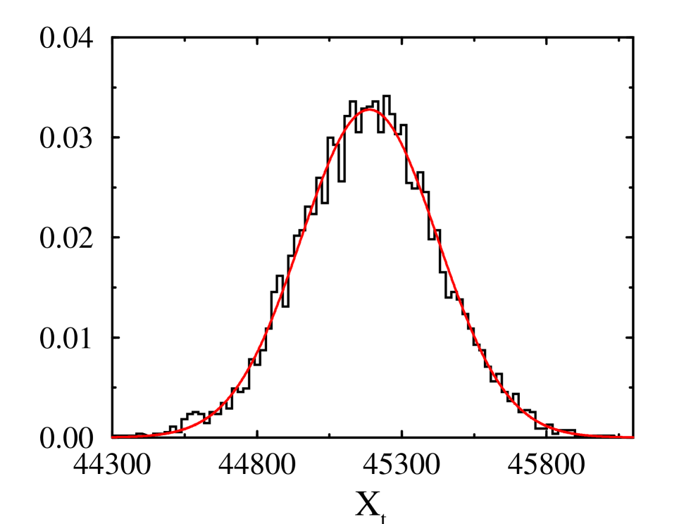
FIG. 1.: Distribution function of the total energy $X_{t}$ for $n=300$. Histogram: from an ensemble of $500$ Gaussian orthogonal matrices of dimension $N=600$; solid line: Gaussian distribution with mean value $\langle X_{t}(300)\rangle$ and variance $\Delta^{2}(300)$ obtained from Eqs.$({\ref{mean}})$ and $({\ref{deldac}})$, respectively.

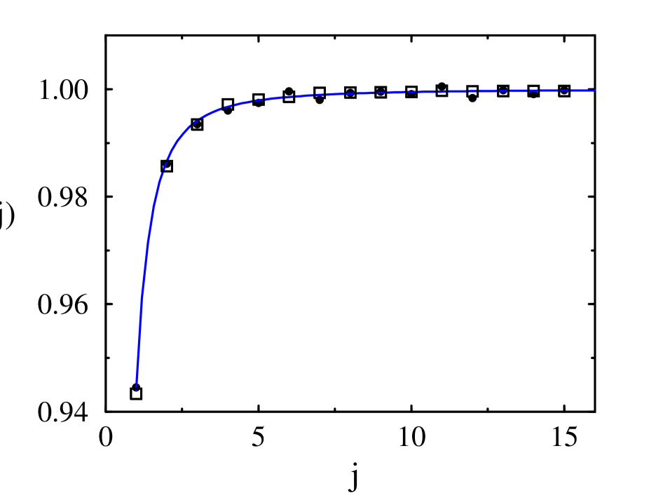
FIG. 2.: Autocorrelation of spacings $I(j)$ for $\beta=2$. Dots: obtained from an ensemble of $500$ Gaussian unitary matrices of dimension $N=500$; solid line: the ansatz $({\ref{ij}})$ for $\beta=2$; squares: computed from the zeros of the Riemann zeta function (taken from [9]).

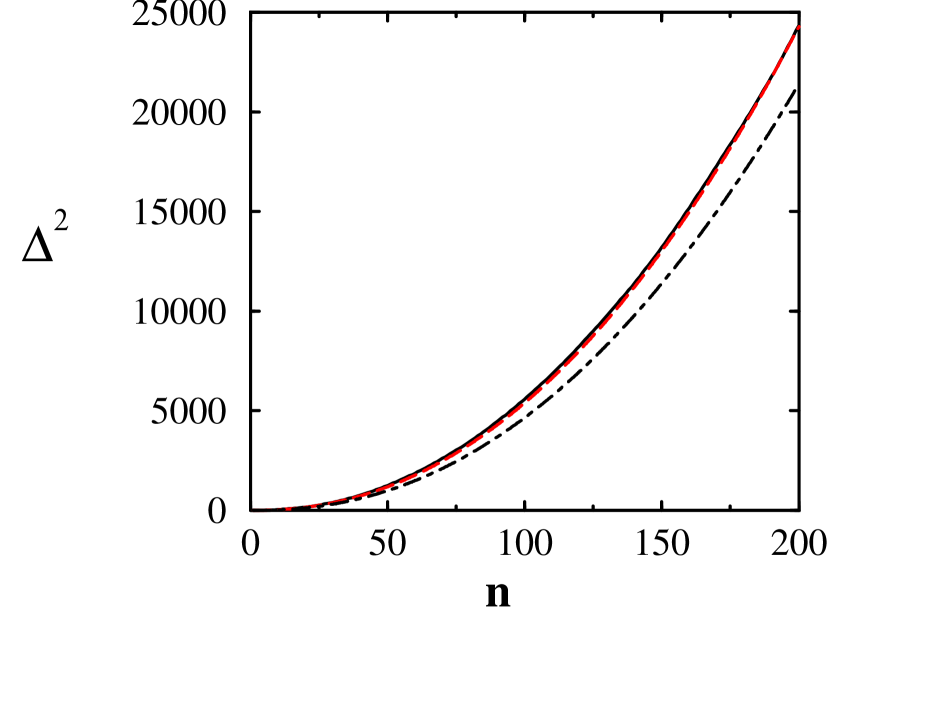
FIG. 3.: Canonical number variance $\Delta^{2}$ for $\beta=1$ as a function of $n$. Solid line: from an ensemble of $500$ Gaussian orthogonal matrices of dimension $N=600$; dashed line: theory (see Eq.$({\ref{deldac}})$); dot-dashed line: leading order term of the same equation.

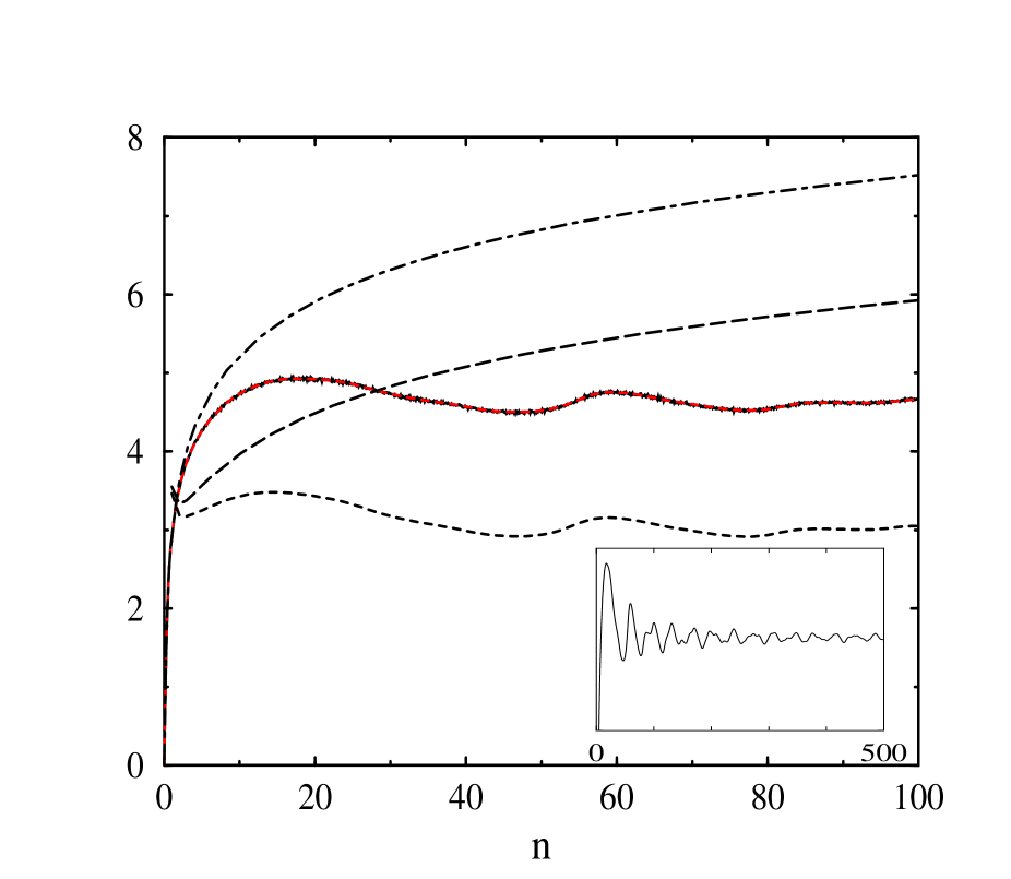
FIG. 4.: Normalized energy variances. Solid line: the normalized grand canonical variance $V_{E}/(n^{2}/2\pi^{2})$ for the zeros of the Riemann zeta function. In this curve the numerical results as well as the theoretical prediction are superimposed, and are almost indistinguishable. The same curve is plotted in a wider range and on an expanded scale in the inset. Dot-dashed line: random matrix result ($\beta=2$) for the normalized grand canonical variance. Dashed line: the normalized canonical variance $\Delta^{2}/(n^{2}/2\pi^{2})$ obtained numerically from the zeros of the Riemann zeta function. Long-dashed line: random matrix result ($\beta=2$, obtained using the ansatz) for the normalized canonical variance. (See text for further explanation).

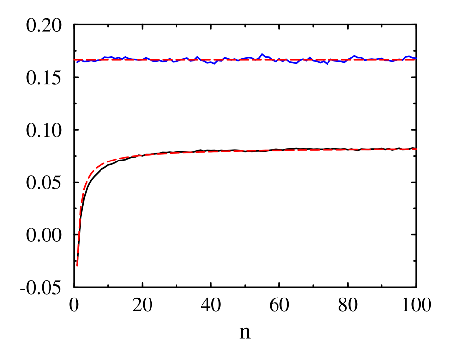
FIG. 5.: Comparison between canonical and grand canonical quantities. The upper solid curve is the difference $\Sigma^{2}-\sigma^{2}$ obtained numerically from the zeros of the Riemann zeta function. The upper dashed horizontal line is at $1/6\approx 0.166$. The lower solid curve is the numerical result for the difference $(V_{E}-\Delta^{2})/n^{2}$ for the same set of zeros. The lower dashed curve displays Eq.(61), which tends to $1/12\approx 0.0833$ for large values of $n$.

REFERENCES

- [1] W. J. Swiatecki, Nucl. Phys. A 574, 233c (1994).
- [2] “Chaos and Quantum Physics” edited by M.-J. Giannoni, A. Voros and J. Zinn-Justin, Les Houches Session LII, (North Holland, Amsterdam, 1991).
- [3] O. Bohigas in Ref.[2]
- [4] H. Politzer, Phys. Rev. B 40, 11197 (1989).
- [5] “Mesoscopic Quantum Physics” edited by E. Akkermans, G. Montambaux, J.-L. Pichard and J. Zinn-Justin, Les Houches Session LXI, (North Holland, Amsterdam, 1995).
- [6] M. L. Mehta, Random Matrices (Academic Press, New York, 1991), 2nd ed.
- [7] M. Abramowitz and I. A. Stegun, Handbook of Mathematical Functions (Dover, New York, 1970).
- [8] J. B. French, P. A. Mello and A. Pandey, Ann. Phys. 113, 277 (1978). T. A. Brody, J. Flores, J. B. French, P. A. Mello, A. Pandey and S. S. M. Wong, Rev. Mod. Phys. 53, 385 (1981); J. B. French, V. K. B. Kota, A. Pandey and S. Tomsovic, Ann. Phys. 181, 198 (1988); A. Pandey, unpublished.
- [9] A. M. Odlyzko, Math. Comp. 48, 273 (1987); AT & T Report, 1989 (unpublished).
- [10] A. Pandey in “Quantum Chaos and Statistical Nuclear Physics” edited by T. H. Seligman and H. Nishioka, Lectures Notes in Physics 263, (Springer Verlag, Berlin, 1986).
- [11] O. Bohigas, R. U. Haq and A. Pandey, Phys. Rev. Lett. 54, 1645 (1985).
- [12] F. J. Dyson and M. L. Mehta, J. Math. Phys. 4, 701 (1963).
- [13] M. Wilkinson, private communication.
- [14] M. V. Berry, Proc. R. Soc. London A400, 229 (1985); see also M. V. Berry in Ref.[2].
- [15] M. C. Gutzwiller, Chaos in Classical and Quantum Mechanics (Springer Verlag, New York, 1990); see also M. C. Gutzwiller, in Ref.[2].
- [16] J. Hannay and A. M. Ozorio de Almeida, J. Phys. A 17, 3429 (1984).
- [17] M. V. Berry, Nonlinearity 1, 399 (1988).
- [18] D. R. Stewart, D. Sprinzak, C. M. Marcus, C. I. Duruöz and J. S. Harris Jr, Science 278, 1784 (1997).
- [19] H. L. Montgomery, Proc. Symp. Pure Math. 24, 181 (1973); D. A. Goldston and H. L. Montgomery, Proc. Conf. at Oklahoma State Univ., edited by A. C. Adolphson et al, 183 (1984).
- [20] E. Bogomolny and J. Keating, Nonlinearity 8, 1115 (1995); ibid 9, 911 (1996); N. Katz and P. Sarnak, preprint Princeton 1997.
- [21] F. J. Dyson, J. Math. Phys. 3, 166 (1962); M. L. Mehta and F. J. Dyson, J. Math. Phys. 4, 713 (1963).
- [22] R. Balian and C. Bloch, Ann. of Phys. 69, 76 (1972); H. Nishioka, K. Hansen and B. R. Mottelson, Phys. Rev. B 42, 9377 (1990).
- [23] J. Pedersen, S. Bjørnholm, J. Borggreen, K. Hansen, T. P. Martin and H. D. Rasmussen, Nature 353, 733 (1991); T. P. Martin, S. Bjørnholm, J. Borggreen, C. Bréchignac, P. Cahuzac, K. Hansen, J. Pedersen, Chem. Phys. Lett. 186, 53 (1991).
- [24] N. Argaman, Y. Imry and U. Smilansky, Phys. Rev. B 47, 4440 (1993).
- [25] G. Montambaux in “Quantum Fluctuations” edited by S. Reynaud, E. Giacobino and J. Zinn-Justin, Les Houches Session LXIII, (North Holland, Amsterdam, 1997).