Numerical Study for the Ground State
of Multi-Orbital Hubbard Models

1 Introduction

In the last dozen years since the discovery of high $T_{\rm c}$ materials ,${}^{\hbox{\immediate{\bf{?}})}}$ $d$ and $f$ electron compounds have been studied extensively with revived interest for the purpose of clarifying effects of strong correlations .${}^{\hbox{\immediate{\bf{?}})}}$ In these systems, competition between spin and orbital components plays an important role leading to complex phenomena such as metal-insulator transitions with spin and/or orbital orderings and fluctuations. Especially, the relevance of orbital degrees of freedom is a subject of recent intensive studies.

The multi-orbital Hubbard model is one of the realistic and simplified models to investigate the interplay between spin and orbital components in the Mott transition. This model is straightforwardly derived from the tight-binding scheme. The explicit form of the Hamiltonian is given by

$${\cal H}={\cal H}_{t}+{\cal H}_{\varepsilon}+{\cal H}_{\mu}+{\cal H}_{U}+{\cal H}_{J},$$ (1)

where

$${\cal H}_{t} = \sum_{ij}\sum_{\nu\nu^{\prime}}t_{ij}^{\nu\nu^{\prime}}\left(c_{i\nu}^{\dagger}c_{j\nu^{\prime}}+{\rm h.c.}\right)$$ (2)

$${\cal H}_{\varepsilon} = \sum_{i}\sum_{\nu}\varepsilon_{\nu}n_{i\nu}$$ (3)

$${\cal H}_{\mu} = -\mu\sum_{i}\sum_{\nu}n_{i\nu}$$ (4)

$${\cal H}_{U} = \sum_{i}\sum_{\nu\leq\nu^{\prime}}U_{\nu\nu^{\prime}}\sum_{\sigma\leq\sigma^{\prime}}\left(1-\delta_{\nu\nu^{\prime}}\delta_{\sigma\sigma^{\prime}}\right)n_{i\nu\sigma}n_{i\nu^{\prime}\sigma^{\prime}}$$ (5)

$${\cal H}_{J} = \sum_{i}\sum_{\nu\neq\nu^{\prime}}J_{\nu\nu^{\prime}}\sum_{\sigma\leq\sigma^{\prime}}\bigl{(}c_{i\nu\sigma}^{\dagger}c_{i\nu^{\prime}\sigma^{\prime}}^{\dagger}c_{i\nu\sigma^{\prime}}c_{i\nu^{\prime}\sigma}+c_{i\nu\sigma}^{\dagger}c_{i\nu\sigma^{\prime}}^{\dagger}c_{i\nu^{\prime}\sigma^{\prime}}c_{i\nu^{\prime}\sigma}\bigr{)}.$$ (6)

Here the operator $c_{i\nu}^{\dagger}$($c_{i\nu}$) creates(annihilates) an electron in the orbital $\nu=1,\cdot\cdot\cdot,N_{\rm C}$ on the site $i=1,\cdot\cdot\cdot,N_{\rm S}$, and $n_{i\nu}\equiv c_{i\nu}^{\dagger}c_{i\nu}$ defines the number operator. The first three terms are one-body terms: ${\cal H}_{t}$ is the hopping term, ${\cal H}_{\varepsilon}$ gives the relative energy level for each orbital and ${\cal H}_{\mu}$ sets the averaged chemical potential $\mu$ which controls the electron filling; We take $\sum_{\nu}\varepsilon_{\nu}=0$. The last two, ${\cal H}_{U}$ and ${\cal H}_{J}$, are two-body interaction terms which are classified as in the conventional way: The former term ${\cal H}_{U}$ is often called the on-site Coulomb term which consists of only diagonal interactions. The latter ${\cal H}_{J}$ is often called the on-site exchange term which contains the Hund coupling and the pair-hopping between orbitals. Note that, in order to keep the rotational symmetry of the two-body interaction, the parameters in Eqs. (5) and (6) are not independent of each other originally .${}^{\hbox{\immediate{\bf{?}},\penalty 1000\hskip 0.91003pt plus 0.70004pt minus 0.70004pt{\bf{?}})}}$ For example, for the twofold $e_{g}$ orbitals in $d$ electron systems whose wave functions are given by $\psi_{i1\sigma}=\left(x^{2}-y^{2}\right)f\left(r\right)$ and $\psi_{i2\sigma}=\frac{1}{\sqrt{3}}\left(3z^{2}-r^{2}\right)f\left(r\right)$, the relation $U_{11}=U_{22}=U_{12}+2J_{12}$ should be satisfied.

As mentioned above, in these multi-orbital systems, fluctuations of both spin and orbital degrees of freedom may compete each other. Various approximations have been examined on this model Eq. (1); mean-field approximations ,${}^{\hbox{\immediate{\bf{?}},\penalty 1000\hskip 0.91003pt plus 0.70004pt minus 0.70004pt{\bf{?}},\penalty 1000\hskip 0.91003pt plus 0.70004pt minus 0.70004pt{\bf{?}},\penalty 1000\hskip 0.91003pt plus 0.70004pt minus 0.70004pt{\bf{?}},\penalty 1000\hskip 0.91003pt plus 0.70004pt minus 0.70004pt{\bf{?}},\penalty 1000\hskip 0.91003pt plus 0.70004pt minus 0.70004pt{\bf{?}})}}$ Gutzwiller approximations ,${}^{\hbox{\immediate{\bf{?}},\penalty 1000\hskip 0.91003pt plus 0.70004pt minus 0.70004pt{\bf{?}},\penalty 1000\hskip 0.91003pt plus 0.70004pt minus 0.70004pt{\bf{?}},\penalty 1000\hskip 0.91003pt plus 0.70004pt minus 0.70004pt{\bf{?}},\penalty 1000\hskip 0.91003pt plus 0.70004pt minus 0.70004pt{\bf{?}},\penalty 1000\hskip 0.91003pt plus 0.70004pt minus 0.70004pt{\bf{?}})}}$ infinite-dimensional approaches ${}^{\hbox{\immediate{\bf{?}},\penalty 1000\hskip 0.91003pt plus 0.70004pt minus 0.70004pt{\bf{?}})}}$ and slave boson approaches .${}^{\hbox{\immediate{\bf{?}},\penalty 1000\hskip 0.91003pt plus 0.70004pt minus 0.70004pt{\bf{?}},\penalty 1000\hskip 0.91003pt plus 0.70004pt minus 0.70004pt{\bf{?}})}}$ However, these approximations in general neglect fluctuations under the competition of various orderings. Although details of the mean-field approximations in these approaches differ each other, they all have a difficulty in describing critical phenomena by nature. A more appropriate treatment which allows studies on fluctuation effects has to be employed in order to discuss critical nature of phase transitions in these complex systems. In fact, the criticality may have relevance to many aspects of physical properties in $d$ or $f$ electron compounds.

In this work, we investigate ground state properties of the multi-orbital Hubbard model by an unbiased method, that is, by the auxiliary field quantum Monte Carlo (QMC) method, recently proposed by the authors .${}^{\hbox{\immediate{\bf{?}})}}$ Several remarkable aspects which cannot be obtained within one-body approximations are elucidated for the one-dimensional systems with doubly degenerate orbitals: First, the characteristic properties as the strongly correlated insulator are elucidated quantitatively for the Mott insulator at half filling; though the charge and spin excitations both have gaps, the charge gap amplitude is much larger than the spin gap. The orbital excitation is gapless, that is, the orbital polarization grows continuously with increasing the level split. Critical properties of the insulator-metal transition are studied by controlling the chemical potential. Analysis on the numerical results based on the hyperscaling hypothesis gives the correlation length exponent $\nu=1/2$, which supports the scaling arguments on the Mott transition in one dimension. The properties under the self doping between two orbitals are also investigated by controlling the level split; the continuous change from the high-spin Mott insulator to the low-spin band insulator is elucidated, where the spin gap amplitude increases sensitively depending on the magnitude of the self doping and become closer to the charge gap.

This paper is organized as follows: In the next section, the auxiliary field QMC technique proposed by the authors is reviewed in detail in a general formalism for arbitrary number of orbital in arbitrary dimension. The matrix representation for this formalism and details of QMC updating are also described explicitly for the readers who are interested in the actual coding procedure. We show that the algorithm does not suffer from the negative sign problem in a non-trivial and physically interesting parameter region of the model defined in Eq. (1). In Sec. 3, we introduce doubly degenerate models to investigate them in the following sections. We also discuss experimental relevance of this doubly degenerate model. In Sec. 4, the ground state properties of this model are investigated by the QMC method in one dimension. Properties of the Mott insulating state at half filling is investigated in terms of correlations of charge, spin and orbital degrees of freedom. The critical properties of insulator-metal transitions controlled by the chemical potential are discussed. For finite level split between two orbitals, effects of self doping are investigated. All these QMC results are discussed in Sec. 5 in detail. Based on the scaling analysis, the critical exponents of the insulator-metal transition by filling control are discussed. The crossover between the Mott insulator in high spin state and the band insulator in low spin state is examined for the level-split control. Finally, Sec. 6 is devoted to summary.

2 Method

Auxiliary field quantum Monte Carlo method is a powerful tool to investigate interacting fermions .${}^{\hbox{\immediate{\bf{?}},\penalty 1000\hskip 0.91003pt plus 0.70004pt minus 0.70004pt{\bf{?}},\penalty 1000\hskip 0.91003pt plus 0.70004pt minus 0.70004pt{\bf{?}},\penalty 1000\hskip 0.91003pt plus 0.70004pt minus 0.70004pt{\bf{?}},\penalty 1000\hskip 0.91003pt plus 0.70004pt minus 0.70004pt{\bf{?}})}}$ In this section, we describe a general algorithm for multi-orbital Hubbard models defined in Eq. (1) for arbitrary number of orbital in arbitrary dimension. This algorithm was developed in the previous letter by the authors .${}^{\hbox{\immediate{?})}}$ We describe it in detail to make this paper be self-contained, especially supplementing the matrix representation and the details of updating procedure.

2.1 Assumption

For the efficiency of the algorithm described below, we assume $U_{\nu\nu^{\prime}}=U$ in Eq. (5). This allows us to factorize the two-body interaction terms Eqs. (5) and (6) into the quadratic forms, as

$${\cal H}_{U} = \frac{U}{2}\sum_{i}\left(n_{i}-N_{\rm C}\right)^{2}+\frac{U}{2}\left(2N_{\rm C}-1\right)\sum_{i}n_{i}-\frac{U}{2}N_{\rm C}^{2}$$ (7)

$${\cal H}_{J} = \sum_{i}\sum_{\nu<\nu^{\prime}}\frac{J_{\nu\nu^{\prime}}}{2}A_{i\nu\nu^{\prime}}^{2}-\sum_{i}\sum_{\nu<\nu^{\prime}}\frac{J_{\nu\nu^{\prime}}}{2}n_{i}.$$ (8)

Here $A_{i\nu\nu^{\prime}}\equiv\sum_{\sigma}A_{i\nu\nu^{\prime}\sigma}\equiv\sum_{\sigma}(c_{i\nu\sigma}^{\dagger}c_{i\nu^{\prime}\sigma}+c_{i\nu^{\prime}\sigma}^{\dagger}c_{i\nu\sigma})$. These factorizations simplify the Hubbard-Stratonovich (HS) transformation as is described below in Eqs. (2.2) and (2.2).

As mentioned in the introduction, the interaction parameters $U_{\nu\nu^{\prime}}$ and $J_{\nu\nu^{\prime}}$ depend on each other to keep the rotational symmetry of the total interaction .${}^{\hbox{\immediate{?},\penalty 1000\hskip 0.91003pt plus 0.70004pt minus 0.70004pt{?})}}$ Our assumption $U_{\nu\nu^{\prime}}=U$ breaks this symmetry. In the following, we further treat the values of $U$ and $J_{\nu\nu^{\prime}}$ as independent parameters as in many previous theoretical studies. We believe that these may not affect the qualitative features of the problem. Note that although our assumptions break the on-site rotational symmetry, the symmetry or dimension of elementary excitations might be closely related to the effective exchange coupling between different sites which strongly depends on the specific form of the hopping matrix $t_{ij}^{\nu\nu^{\prime}}$ as well as the electron filling or the orbital degeneracy; the following algorithm is applicable to any type of $t_{ij}^{\nu\nu^{\prime}}$.

2.2 Basic formalism

There exist two schemes in the auxiliary field QMC technique; one is for finite temperatures and the other is for the ground state. In the finite temperature calculation, we need to calculate the partition function, $Z={\rm Tr}\exp\left(-\beta{\cal H}\right)$ .${}^{\hbox{\immediate{?},\penalty 1000\hskip 0.91003pt plus 0.70004pt minus 0.70004pt{?},\penalty 1000\hskip 0.91003pt plus 0.70004pt minus 0.70004pt{?})}}$ Compared with this, for the ground state calculation which is often called the projection quantum Monte Carlo method ,${}^{\hbox{\immediate{?},\penalty 1000\hskip 0.91003pt plus 0.70004pt minus 0.70004pt{?})}}$ it is necessary to calculate the density matrix, $\rho\left(\beta;\phi\right)\equiv\langle\phi|\exp\left(-\beta{\cal H}\right)|\phi\rangle$, where $|\phi\rangle$ is a trial wave function non-orthogonal to the ground state. Below, we describe the basic formalism to calculate the common quantity $\exp\left(-\beta{\cal H}\right)$ in both schemes.

First step is the Suzuki-Trotter decomposition into the $M=\beta/\Delta\tau$ slices in the imaginary time direction .${}^{\hbox{\immediate{\bf{?}},\penalty 1000\hskip 0.91003pt plus 0.70004pt minus 0.70004pt{\bf{?}},\penalty 1000\hskip 0.91003pt plus 0.70004pt minus 0.70004pt{\bf{?}})}}$ Then we obtain

$$e^{-\beta{\cal H}}=\left(e^{-\Delta\tau{\cal H}_{t}/2}e^{-\Delta\tau{\cal H}_{\varepsilon}/2}e^{-\Delta\tau{\cal H}_{\mu}}e^{-\Delta\tau{\cal H}_{U}}e^{-\Delta\tau{\cal H}_{J}}e^{-\Delta\tau{\cal H}_{\varepsilon}/2}e^{-\Delta\tau{\cal H}_{t}/2}\right)^{M}+O\left(\Delta\tau^{2}\right).$$ (9)

Next, in order to derive a one-body expression, we replace the two-body interaction terms ${\cal H}_{U}$ and ${\cal H}_{J}$ with non-interacting ones by introducing the HS transformation .${}^{\hbox{\immediate{\bf{?}},\penalty 1000\hskip 0.91003pt plus 0.70004pt minus 0.70004pt{\bf{?}})}}$ The general formula of the discrete HS transformation we use here is given by ${}^{\hbox{\immediate{?})}}$

$$\exp\left(-\Delta\tau\theta f^{2}\right)=\sum_{l,s=\pm 1}\frac{\gamma_{l}}{4}\exp\left({\rm i}s\eta_{l}\sqrt{\alpha}f\right)+O(\Delta\tau^{4}),$$ (10)

where $\gamma_{l}\equiv 1+\frac{\sqrt{6}}{3}l,\eta_{l}\equiv\sqrt{2(3-\sqrt{6}l)}$ and $\alpha\equiv\Delta\tau\theta\geq 0$. Applying this formula to Eqs. (7) and (8), we obtain

$$\exp\Bigl{(}-\Delta\tau\frac{U}{2}\sum_{i}\left(n_{i}-N_{\rm C}\right)^{2}\Bigr{)}$$

$$= \prod_{i}\biggl{[}\sum_{l_{1i},s_{1i}=\pm 1}\frac{\gamma_{l_{1i}}}{4}\exp\left\{{\rm i}s_{1i}\eta_{l_{1i}}\sqrt{\alpha_{1}}\left(n_{i}-N_{\rm C}\right)\right\}\biggr{]}+O(\Delta\tau^{4})$$

$$\exp\Bigl{(}-\Delta\tau\sum_{i}\sum_{\nu<\nu^{\prime}}\frac{J_{\nu\nu^{\prime}}}{2}A_{i\nu\nu^{\prime}}^{2}\Bigr{)}$$

$$= \prod_{i}\prod_{\nu<\nu^{\prime}}\biggl{[}\sum_{l_{2i}^{\nu\nu^{\prime}},s_{2i}^{\nu\nu^{\prime}}=\pm 1}\frac{\gamma_{l_{2i}^{\nu\nu^{\prime}}}}{4}\exp\left\{{\rm i}s_{2i}^{\nu\nu^{\prime}}\eta_{l_{2i}^{\nu\nu^{\prime}}}\sqrt{\alpha_{2}^{\nu\nu^{\prime}}}A_{i\nu\nu^{\prime}}\right\}\biggr{]}+O(\Delta\tau^{4}),$$

where $\alpha_{1}=\Delta\tau U/2\geq 0$ and $\alpha_{2}^{\nu\nu^{\prime}}=\Delta\tau J_{\nu\nu^{\prime}}/2\geq 0$.

Of course, the way to decompose the two-body interaction terms, that is, the type of the HS transformation is not unique. The advantage of our scheme with Eq. (10) lies in the fact that it brings the non-trivial parameter regions where the negative sign difficulty does not exist. We discuss this point in Sec. 2.5 in detail.

We apply these decompositions to each Suzuki-Trotter slice in Eq. (9). Then, the one-body expression is given as

$$\exp\left(-\beta{\cal H}\right)=\sum_{\{l_{1}s_{1}l_{2}^{\nu\nu^{\prime}}s_{2}^{\nu\nu^{\prime}}\}}\prod_{\sigma}\prod_{m=1}^{M}\left[w_{t\sigma}w_{\varepsilon\sigma}w_{\mu\sigma}w_{U\sigma}(l_{1}(m),s_{1}(m))w_{J\sigma}(l_{2}(m),s_{2}(m))w_{\varepsilon\sigma}w_{t\sigma}\right]$$ (13)

with

$$w_{t\sigma} = \prod_{i=1}^{N_{\rm S}}\exp\left(-\Delta\tau{\cal H}_{t\sigma}/2\right)$$ (14)

$$w_{\varepsilon\sigma} = \prod_{i=1}^{N_{\rm S}}\prod_{\nu}\exp\left(-\Delta\tau\varepsilon_{\nu}n_{i\nu\sigma}/2\right)$$ (15)

$$w_{\mu\sigma} = \left[-\mu+\frac{U}{2}\left(2N_{\rm C}-1\right)+\sum_{\nu<\nu^{\prime}}\frac{J_{\nu\nu^{\prime}}}{2}\right]\sum_{i}n_{i\sigma}$$ (16)

$$w_{U\sigma} = \prod_{i=1}^{N_{\rm S}}\frac{\sqrt{\gamma_{l_{1i}}}}{2}\exp\Bigl{\{}{\rm i}s_{1i}\eta_{l_{1i}}\sqrt{\alpha_{1}}\Bigl{(}n_{i\sigma}-\frac{N_{\rm C}}{2}\Bigr{)}\Bigr{\}}$$ (17)

$$w_{J\sigma} = \prod_{{i=1}\atop{\nu<\nu^{\prime}}}^{N_{\rm S}}\frac{\sqrt{\gamma_{l_{2i}^{\nu\nu^{\prime}}}}}{2}\exp\left({\rm i}s_{2i}^{\nu\nu^{\prime}}\eta_{l_{2i}^{\nu\nu^{\prime}}}\sqrt{\alpha_{2}^{\nu\nu^{\prime}}}A_{i\nu\nu^{\prime}\sigma}\right).$$ (18)

The product of Eqs. (2.2) and (2.2) over all the Suzuki-Trotter slices amounts to the systematic error of $O(\Delta\tau^{3})$ which is negligible because it is higher order than the other systematic errors from the Suzuki-Trotter decomposition in Eq. (9). In Appendix A, we discuss the behavior of these errors in detail.

2.3 Matrix representation

A matrix representation for the above expressions is helpful in an actual coding. We derive it explicitly here in the case of the ground state algorithm for discussions in the following part. The following representations can easily be applied to the finite temperature calculation only with slight modifications.

We use a trial wave function $|\phi\rangle=|\phi^{\uparrow}\rangle\otimes|\phi^{\downarrow}\rangle$ with

$$|\phi^{\sigma}\rangle=\prod_{j=1}^{N_{\rm e}^{\sigma}}\left(\sum_{i=1}^{N}\left(\Phi_{\sigma}\right)_{ij}c_{i\sigma}^{\dagger}\right)|0\rangle,$$ (19)

where $N_{\rm e}^{\sigma}$ is the electron number with $\sigma$ spin; $N=N_{\rm S}\times N_{\rm C}$; and $|0\rangle$ is the vacuum. Then, the matrix representation for the density matrix in the canonical calculation is given as

$$\rho\left(\beta;\phi\right)=\sum_{\{l_{1}s_{1}l_{2}^{\nu\nu^{\prime}}s_{2}^{\nu\nu^{\prime}}\}}W_{\uparrow}\left(\{l_{1}s_{1}l_{2}^{\nu\nu^{\prime}}s_{2}^{\nu\nu^{\prime}}\};\beta;\phi\right)W_{\downarrow}\left(\{l_{1}s_{1}l_{2}^{\nu\nu^{\prime}}s_{2}^{\nu\nu^{\prime}}\};\beta;\phi\right),$$ (20)

where

$$W_{\sigma}=C_{\{l_{1}s_{1}l_{2}^{\nu\nu^{\prime}}s_{2}^{\nu\nu^{\prime}}\}}\det\left[{}^{t}\Phi_{\sigma}B_{\{l_{1}s_{1}l_{2}^{\nu\nu^{\prime}}s_{2}^{\nu\nu^{\prime}}\}}\left(\beta,0\right)\Phi_{\sigma}\right].$$ (21)

Here,

$$C_{\{l_{1}s_{1}l_{2}^{\nu\nu^{\prime}}s_{2}^{\nu\nu^{\prime}}\}}=\prod_{m=1}^{M}\prod_{i=1}^{N}\frac{\sqrt{\gamma_{l_{1i}\left(m\right)}\gamma_{l_{2i}^{\nu_{i}{\nu_{i}}^{\prime}}\left(m\right)}}}{4}\exp\left(-{\rm i}s_{1i}\left(m\right)\eta_{l_{1i}\left(m\right)}\sqrt{\alpha_{1}}\frac{N_{C}}{2}\right)$$ (22)

$$B_{\{l_{1}s_{1}l_{2}^{\nu\nu^{\prime}}s_{2}^{\nu\nu^{\prime}}\}}\left(\tau_{2},\tau_{1}\right)=\prod_{m=m_{1}+1}^{m_{2}}b\left(m\right),$$ (23)

where $\tau_{i}=m_{i}\Delta\tau$ $(i=1,2)$ and

$$b\left(m\right)=e^{-\frac{\Delta\tau}{2}T}e^{L}e^{D(m)}e^{E(m)}e^{L}e^{-\frac{\Delta\tau}{2}T}.$$ (24)

Here $T,L,D$ and $E$ are $N\times N$ matrices given by

$$\sum_{\tilde{i},\tilde{j}}^{N}c_{\tilde{i}\sigma}^{\dagger}\left(T\right)_{\tilde{i}\tilde{j}}c_{\tilde{j}\sigma} = {\cal H}_{t\sigma}$$ (25)

$$\left(L\right)_{\tilde{i}\tilde{j}} = -\frac{\Delta\tau}{2}\varepsilon_{\nu_{i}}\delta_{\tilde{i}\tilde{j}}$$ (26)

$$\left(D\right)_{\tilde{i}\tilde{j}} = {\rm i}s_{1{i}}\left(m\right)\eta_{l_{1{i}}\left(m\right)}\sqrt{\alpha_{1}}\delta_{ij}$$ (27)

$$\left(E\right)_{\tilde{i}\tilde{j}} = \sum_{\nu<\nu^{\prime}}{\rm i}s_{2{i}}^{\nu\nu^{\prime}}\left(m\right)\eta_{l_{2{i}}^{\nu\nu^{\prime}}\left(m\right)}\sqrt{\alpha_{2}^{\nu\nu^{\prime}}}\delta_{ij}\left(\delta_{\nu_{i}\nu}\delta_{\nu_{j}\nu^{\prime}}+\delta_{\nu_{j}\nu}\delta_{\nu_{i}\nu^{\prime}}\right).$$ (28)

In Eqs. (25) $\sim$ (28), the index $\tilde{i}$ contains the site and orbital indices, $\tilde{i}\equiv\left(i,\nu_{i}\right)$. $\delta_{ij}$ is the Cronecker’s delta function.

2.4 Updating

The summation over $\{l_{1}s_{1}l_{2}^{\nu\nu^{\prime}}s_{2}^{\nu\nu^{\prime}}\}$ in Eq. (20) is statistically sampled by the Monte Carlo technique. In the ground state algorithm, a change $\{l,s\}=\{l_{1}s_{1}l_{2}^{\nu\nu^{\prime}}s_{2}^{\nu\nu^{\prime}}\}\rightarrow\{l^{\prime},s^{\prime}\}=\{l^{\prime}_{1}s^{\prime}_{1}{l^{\prime}}_{2}^{\nu\nu^{\prime}}{s^{\prime}}_{2}^{\nu\nu^{\prime}}\}$ is accepted by the probability

$$P=\left|\frac{\prod_{\sigma}W_{\sigma}\left(\{l^{\prime},s^{\prime}\}\right)}{\prod_{\sigma}W_{\sigma}\left(\{l,s\}\right)}\right|.$$ (29)

The probability Eq. (29), which is called the acceptance ratio, may be rewritten into more simple form by using the single-particle Green function .${}^{\hbox{\immediate{?})}}$ For a change from $\{l_{\lambda i}\left(m\right),s_{\lambda i}\left(m\right)\}$ to $\{\bar{l}_{\lambda i}\left(m\right),\bar{s}_{\lambda i}\left(m\right)\}$ $(\lambda=1,2)$, the acceptance ratio $P$ is given as

$$P=\left|\tilde{C}_{\lambda}\prod_{\sigma}\det\left[I+\Delta_{\lambda}G_{\sigma}\left(m\right)\right]\right|,$$ (30)

where $I$ is the $N\times N$ unit matrix,

$$\tilde{C}_{1} = \sqrt{\frac{\gamma_{\bar{l}_{1i}\left(m\right)}}{\gamma_{l_{1i}\left(m\right)}}}\exp\left[-{\rm i}\sqrt{\alpha_{1}}\frac{N_{\rm C}}{2}\left(\bar{s}_{1i}\left(m\right)\eta_{\bar{l}_{1i}\left(m\right)}-s_{1i}\left(m\right)\eta_{l_{1i}\left(m\right)}\right)\right]$$ (31)

$$\tilde{C}_{2} = \sqrt{\gamma_{\bar{l}_{2i}^{\nu_{i}{\nu_{i}}^{\prime}}\left(m\right)}/\gamma_{l_{2i}^{\nu_{i}{\nu_{i}}^{\prime}}\left(m\right)}}.$$ (32)

$\Delta_{\lambda}$ are sparse $N\times N$ matrices with only non-zero elements,

$$\left(\Delta_{\lambda}\right)_{\left(i,\nu_{i}\right)\left(i,{\nu_{i}}^{\prime}\right)}=\left(\Gamma_{\lambda}\right)_{\left(i,\nu_{i}\right)\left(i,{\nu_{i}}^{\prime}\right)}-\delta_{\nu_{i}{\nu_{i}}^{\prime}}$$ (33)

with

$$\left(\Gamma_{1}\right)_{\tilde{i}\tilde{i}} = \exp\left[{\rm i}\sqrt{\alpha_{1}}\left(\bar{s}_{1i}\left(m\right)\eta_{\bar{l}_{1i}\left(m\right)}-s_{1i}\left(m\right)\eta_{l_{1i}\left(m\right)}\right)\right]$$ (34)

$$\left(\Gamma_{2}\right)_{\left(i,\nu_{i}\right)\left(i,{\nu_{i}}^{\prime}\right)} = \frac{\exp\left[{\rm i}\sqrt{\alpha_{2}^{\nu_{i}{\nu_{i}}^{\prime}}}\bar{s}_{2i}^{\nu_{i}{\nu_{i}}^{\prime}}\left(m\right)\eta_{\bar{l}_{2i}^{\nu_{i}{\nu_{i}}^{\prime}}\left(m\right)}\right]}{\exp\left[{\rm i}\sqrt{\alpha_{2}^{\nu_{i}{\nu_{i}}^{\prime}}}s_{2i}^{\nu_{i}{\nu_{i}}^{\prime}}\left(m\right)\eta_{l_{2i}^{\nu_{i}{\nu_{i}}^{\prime}}\left(m\right)}\right]}.$$ (35)

Here, the single-particle Green function at the $m$-th imaginary time slice is calculated by

$$G_{\sigma}\left(m\right)=\Theta_{R}^{\sigma}\left(m\right)\left({}^{t}\Phi_{\sigma}B\left(\beta,0\right)\Phi_{\sigma}\right)^{-1}{}^{t}\Theta_{L}^{\sigma}\left(m\right),$$ (36)

where

$$\Theta_{R}^{\sigma}\left(m\right) = e^{D\left(m\right)}e^{E\left(m\right)}e^{L}e^{-\Delta\tau T/2}B\left(\left(m-1\right)\Delta\tau,0\right)\Phi_{\sigma}$$ (37)

$${}^{t}\Theta_{L}^{\sigma}\left(m\right) = {}^{t}\Phi_{\sigma}B\left(\beta,\left(m+1\right)\Delta\tau\right)e^{-\Delta\tau T/2}e^{L}.$$ (38)

Note that $W_{\sigma}=C\det\left[{}^{t}\Theta_{L}^{\sigma}\Theta_{R}^{\sigma}\right]$.

If the change of the HS variables is accepted, the updated Green function $\bar{G}$ for $\{\bar{l}_{\lambda i}\left(m\right),\bar{s}_{\lambda i}\left(m\right)\}$ is calculated from the old one $G$ for $\{l_{\lambda i}\left(m\right),s_{\lambda i}\left(m\right)\}$ as,

$$\bar{G}_{\sigma}=\left(I+\Delta_{\lambda}\right)\tilde{G}_{\sigma},$$ (39)

where

$$\left(\tilde{G}_{\sigma}\right)_{\tilde{j}\tilde{k}} = \left(G_{\sigma}\right)_{\tilde{j}\tilde{k}}-\sum_{\nu_{i}{\nu_{i}}^{\prime}}\left(G_{\sigma}\right)_{\tilde{j}\left(i,\nu_{i}\right)}\left(\Gamma_{\lambda}\right)_{\nu_{i}{\nu_{i}}^{\prime}}\sum_{\nu}\left(Q^{-1}\right)_{{\nu_{i}}^{\prime}\nu}\left(G_{\sigma}\right)_{\left(i,\nu\right)\tilde{k}}.$$ (40)

The $N_{\rm C}\times N_{\rm C}$ matrix $Q$ is defined as

$$\left(Q\right)_{\nu_{i}{\nu_{i}}^{\prime}} = \delta_{\nu_{i}{\nu_{i}}^{\prime}}+\sum_{\nu}\left(G_{\sigma}\right)_{\left(i,\nu_{i}\right)\left(i,\nu\right)}\left(\Delta_{\lambda}\right)_{\left(i,\nu\right)\left(i,{\nu_{i}}^{\prime}\right)}.$$ (41)

To summarize, the actual MC sampling goes as follows: Calculate the single-particle Green function for given HS variables. Generate a change of a HS variable and calculate the acceptance ratio Eq. (30) by using the Green function. If the change is accepted, recalculate the Green function by Eq. (39). Repeat this procedure for all the sites and all the imaginary time slices. This amounts to the one MC sweep.

In general, the weight for each Monte Carlo sample $W_{\uparrow}W_{\downarrow}$ can have a negative value, which leads to the negative sign problem .${}^{\hbox{\immediate{\bf{?}},\penalty 1000\hskip 0.91003pt plus 0.70004pt minus 0.70004pt{\bf{?}},\penalty 1000\hskip 0.91003pt plus 0.70004pt minus 0.70004pt{\bf{?}},\penalty 1000\hskip 0.91003pt plus 0.70004pt minus 0.70004pt{\bf{?}},\penalty 1000\hskip 0.91003pt plus 0.70004pt minus 0.70004pt{\bf{?}},\penalty 1000\hskip 0.91003pt plus 0.70004pt minus 0.70004pt{\bf{?}},\penalty 1000\hskip 0.91003pt plus 0.70004pt minus 0.70004pt{\bf{?}},\penalty 1000\hskip 0.91003pt plus 0.70004pt minus 0.70004pt{\bf{?}},\penalty 1000\hskip 0.91003pt plus 0.70004pt minus 0.70004pt{\bf{?}})}}$ The difficulty caused by the negative sign depends on details of the systems; the long-range hopping, the electron density and the dimensionality of the system. In Appendix B, we discuss how the negative-sign samples appear in our framework briefly for a specific model which is introduced in Sec. 3.1.

2.5 Cases free from the negative sign problem

Here we discuss non-trivial conditions on parameters in multi-orbital models which are completely free from the negative sign problem .${}^{\hbox{\immediate{?})}}$

Negative-sign samples do not appear when a system keeps the particle-hole symmetry. There, it is easily shown that the weight of the Monte Carlo sample for the up-spin is just the complex conjugate of that for the down-spin; $W_{\uparrow}W_{\downarrow}=|W_{\uparrow}|^{2}\geq 0$. In multi-orbital cases, the symmetry about orbital indices provides us with the following conditions i $\sim$ iv to hold the particle-hole symmetry:

i) The system is at half filling; the electron density satisfies

$$n\equiv\frac{N_{\rm e}^{\uparrow}+N_{\rm e}^{\downarrow}}{N_{\rm S}}=N_{\rm C}.$$ (42)

ii) The energy levels split symmetrically around the Fermi energy;

$$\varepsilon_{\nu}=-\varepsilon_{\bar{\nu}},$$ (43)

where ${\bar{\nu}}\equiv N_{\rm C}-\nu+1$.

iii) The intra-site exchange couplings satisfy a particular relation;

$$J_{\nu\nu^{\prime}}=\delta_{{\bar{\nu}}\nu^{\prime}}J_{\nu}.$$ (44)

iv) The hopping integrals satisfy a special condition;

$$t_{ij}^{\nu\nu^{\prime}}=(-1)^{|i-j|}t_{ij}^{{\bar{\nu^{\prime}}}{\bar{\nu}}},$$ (45)

where $|i-j|$ is the Manhattan distance between site $i$ and $j$. For these conditions, the particle-hole transformation to ensure the positivity of Monte Carlo weights is given by

$$c_{i\nu\uparrow} \rightarrow (-1)^{i}{\tilde{c}}_{i{\bar{\nu}}\uparrow}^{\dagger}$$ (46)

$$c_{i\nu\downarrow} \rightarrow {\tilde{c}}_{i\nu\downarrow}.$$ (47)

Here, we illustrate these conditions i $\sim$ iv expressed by Eqs. (42) $\sim$ (45) and their significance by using a heuristic example. We consider here a system with doubly degenerate orbitals in two dimensions. An effect of finite $\varepsilon\equiv\varepsilon_{1}=-\varepsilon_{2}$ is easily understood in the case of non-interacting system with only the nearest neighbor hoppings which are diagonal in orbital indices. Dispersions of two orbitals are separated by $2\varepsilon$ around the Fermi energy, therefore, a self doping occurs between two orbitals. This leads to difference of the Fermi volume and changes of the nesting behavior as shown in Fig. 1 (b). Next, we discuss an effect of long-range hopping. We consider here the next-nearest neighbor hopping $t_{\langle\langle ij\rangle\rangle}^{11}=-t_{\langle\langle ij\rangle\rangle}^{22}=t^{\prime}\geq 0$, where $\langle\langle ij\rangle\rangle$ denotes that the sites $i$ and $j$ are the next-nearest neighbor pairs. Note that the change in this parameter also controls the bandwidth. Fig. 1 (c) shows an effect of this type of long-range hopping. In this case also, a self doping between two orbitals occurs. In contrast to the case of a finite $\varepsilon$ in Fig. 1 (b), it should be noted that long-range hoppings can change the shapes of the Fermi surfaces as shown in Fig. 1 (c).

It should be stressed here that these changes by $\varepsilon$ or $t^{\prime}$ do not break the perfect nesting property with the nesting vector $(\pi,\pi)$, because the Fermi surface of the orbital $\nu=1$ coincides with that of $\nu=2$ by the shift of the momentum $(\pi,\pi)$. In other words, if the particle-hole symmetry holds, all the $k$-points on the Fermi surface are nested with those on the Fermi surface of the other orbital. This may lead to the Umklapp scattering which may let the system be insulating when we switch on the interactions. However, by these changes, the symmetry about the orbital index which exists at $\varepsilon=t^{\prime}=0$ is broken and the self-doping is realized. It is a non-trivial problem how the nature of the Mott insulator at $\varepsilon=t^{\prime}=0$ changes by controlling $\varepsilon$ or $t^{\prime}$.

Especially, the control of the level split $\varepsilon$ contains an interesting problem. The system exhibits two different states as limiting cases; The Mott insulator at $\varepsilon=0$ and the band insulator at $\varepsilon=\infty$. The former is a consequence of the strong correlation, that is, it does not appear in the non-interacting case. The latter is a trivial insulator which has the same energy gap in both spin and orbital channels as the particle-hole excitation gap. It deserves studying how the spin and orbital states change with the level split. In Sec. 4.4 and 5.2, we investigate this problem in detail.

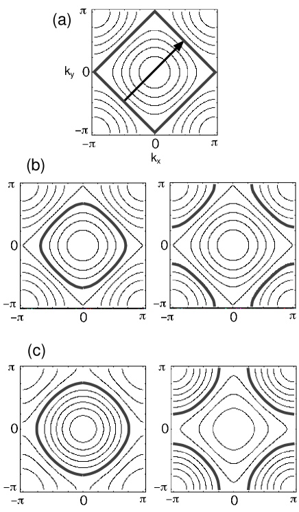
Fig.  1: Effects of a particular type of the level split or long-range hopping at half filling (See text). (a) Energy contour curves for the case with only orbitally-diagonal hopping between nearest neighbor pairs. The arrow represents the nesting vector $(\pi,\pi)$. (b) Energy contour curves for each orbital $\nu=1$(left) and $2$(right) when the level split $\varepsilon=0.8t$. (c) Energy contour curves for each orbital $\nu=1$(left) and $2$(right) when the next-nearest neighbor hopping $t^{\prime}=0.2t$. In all the figures, the Fermi surfaces are denoted by the bold black curves.

3 Doubly Degenerate Models

In the following sections, we concentrate on the doubly degenerate cases of the Hamiltonian Eq. (1). By the auxiliary field QMC technique introduced in Sec. 2, the ground state properties of doubly degenerate systems are investigated in one dimension. In Sec. 3.1, we define the explicit form of the Hamiltonian and give some remarks on basic properties of it. Experimental relevance of our model is discussed in Sec. 3.2.

3.1 Hamiltonian and some remarks

We consider in the following doubly degenerate Hubbard models, given by Eq. (1) with $N_{\rm C}=2$. For simplicity, we take into account only nearest neighbor hoppings which are diagonal about orbital indices. The level split between orbital $\nu=1$ and $2$ is taken to satisfy the condition Eq. (43). Moreover, as described in Sec. 2.1, for the convenience of the HS transformation in the auxiliary field technique, we take uniform values of $U_{\nu\nu^{\prime}}$ irrespective of orbital indices. Then, the explicit forms of Hamiltonian are given by

$${\cal H}_{t} = -t\sum_{\nu=1}^{2}\sum_{\sigma}\sum_{\langle ij\rangle}c_{i\nu\sigma}^{\dagger}c_{j\nu\sigma}+{\rm h.c.}$$ (48)

$${\cal H}_{\varepsilon} = \varepsilon\sum_{i}\left(n_{i1}-n_{i2}\right)$$ (49)

$${\cal H}_{U} = U\sum_{i}\sum_{\nu\leq\nu^{\prime}=1}^{2}\sum_{\sigma\leq\sigma^{\prime}}\left(1-\delta_{\nu\nu^{\prime}}\delta_{\sigma\sigma^{\prime}}\right)n_{i\nu\sigma}n_{i\nu^{\prime}\sigma^{\prime}}$$ (50)

$${\cal H}_{J} = J\sum_{i}\sum_{\nu\neq\nu^{\prime}=1}^{2}\sum_{\sigma\leq\sigma^{\prime}}\bigl{(}c_{i\nu\sigma}^{\dagger}c_{i\nu^{\prime}\sigma^{\prime}}^{\dagger}c_{i\nu\sigma^{\prime}}c_{i\nu^{\prime}\sigma}+c_{i\nu\sigma}^{\dagger}c_{i\nu\sigma^{\prime}}^{\dagger}c_{i\nu^{\prime}\sigma^{\prime}}c_{i\nu^{\prime}\sigma}\bigr{)},$$ (51)

where summations on $\langle ij\rangle$ are over the nearest neighbor sites. In the following, only half-filled cases are discussed. Therefore, the particle-hole symmetry holds for all the parameter regions, which ensures the absence of the negative sign difficulty in the Monte Carlo calculations as explained in Sec. 2.5.

Although this model represents a limited case of the general Hamiltonian (1), it still keeps many general aspects and serves our purposes. The hopping diagonal in orbital indices does not cause the mixing of two orbitals, while the last term ${\cal H}_{J}$ contains off-diagonal elements which mix the orbitals $\nu=1$ and $2$. Note that the second term in Eq. (51) which denotes the pair hopping term between two orbitals has been looked over in most of previous works, although this term is naturally derived from the tight-binding scheme as mentioned in Sec. 1.

Our model Eqs. (48) $\sim$ (51) is easily shown to have two insulating states as particular limits: (a) When $U,J\gg t$ at $\varepsilon=0$, the system is the Mott insulator. The energy gap, which is called the Mott gap, becomes $2U$. (b) When $\varepsilon\rightarrow\infty$ with finite $U,J$ and $t$, since all the electrons fully occupy the orbital $\nu=2$, the system becomes the band insulator.

For finite values of $U$ and $J$, the system is expected to be in the Mott insulating state at $\varepsilon=0$ because of the perfect nesting property. In the following, the ground state properties of our model are discussed by changing the chemical potential $\mu$ and the level split $\varepsilon$ from this Mott insulator. By the former control, we investigate the critical nature of the Mott transition. The latter control, from a consideration in the weak correlation regime as detailed in Sec. 2.5, leads to the self doping between two orbitals, which affects spin and/or orbital states in the Mott insulator. We discuss how the Mott insulator at $\varepsilon=0$ crossovers into the band insulator at $\varepsilon=\infty$ by this self doping in detail.

3.2 Experimental situation

In this part, we discuss experimental situations where our model Eqs. (48) $\sim$ (51) may have relevance. As mentioned in the previous section, the keywords of our model are two active orbitals and half filling.

In $d$ electron systems, the fivefold energy levels of the bare $d$ electron is split by the crystal field. For example, in the octahedral or tetrahedral surroundings, the fivefold degeneracy splits into the twofold $e_{g}$ and the threefold $t_{2g}$ orbitals. For the former octahedral arrangement, the $e_{g}$ levels have higher energy than the $t_{2g}$ ones, and for the latter tetrahedral case, upside down. Therefore, the on-site situation of our model is realized for the $d^{8}$ configuration in the octahedral surroundings or the $d^{2}$ configuration in the tetrahedral surroundings. For both situations, the level split between the active twofold orbitals is easily induced by the deformation of the surrounding ligands. This deformation is considered to be caused by the lattice structure itself or the effect of the external pressure.

There are several materials which consist of the above-mentioned $d^{8}$ units in the octahedral ligand field. One realization is the group of Ni²⁺ compounds; KNiF₃, K₂NiF₄, ${}^{\hbox{\immediate{\bf{?}})}}$ Ni(C₂H₈N₈)₂NO₂(ClO₄) (NENP) ${}^{\hbox{\immediate{\bf{?}},\penalty 1000\hskip 0.91003pt plus 0.70004pt minus 0.70004pt{\bf{?}})}}$ and its related materials or Y₂BaNiO₅ .${}^{\hbox{\immediate{\bf{?}},\penalty 1000\hskip 0.91003pt plus 0.70004pt minus 0.70004pt{\bf{?}})}}$ Since in the following sections we investigate our model in one dimension, we focus here the last two materials, NENP or Y₂BaNiO₅. These materials have one-dimensional network of the octahedrons which may be described by our model Hamiltonian when we forget the ligands. In these systems, however, the hopping matrix is not an orbital-diagonal one like Eq. (48); It may depend on the orbital indices according to each lattice structure. Moreover, the level split by the deformation of octahedrons may generally take place in a complicated way, not in a symmetric form like Eq. (49). Nevertheless, our simple model Eqs. (48) $\sim$ (51) serves to investigate the universal aspects of doubly degenerate systems not depending on details of parameters as mentioned in the previous section. In Sec. 5, our numerical results will be examined from this point of view and the relevance on the experimental situations will be discussed.

4 QMC Results

In this section, the ground state properties of the doubly degenerate model defined in Sec. 3.1 are investigated by the auxiliary field QMC technique detailed in Sec. 2. First, numerical details in the QMC calculations are mentioned, followed by results of this model.

4.1 Details of computations

The model defined in Sec. 3.1 is investigated in one dimension under the periodic boundary condition. The QMC data are obtained from $1,000\sim 10,000$ sample averages for the state $\exp(-\frac{\beta}{2}{\cal H})|\phi\rangle$, where we take $\beta t=10\sim 50$ depending on each situation to obtain converged values in the ground state. Measurements are divided into five blocks and the statistical error of a quantity is estimated by the variance among these five blocks. In order to accelerate the convergence ,${}^{\hbox{\immediate{\bf{?}})}}$ we use the unrestricted Hartree-Fock ground state as a trial state $|\phi\rangle$. The QMC calculations are mainly done for $U=4J=3t$. We set $\Delta\tau t=0.04$ for these interaction parameters, which ensures within the statistical errors the convergence to the limit $\Delta\tau\rightarrow 0$ for all the physical quantities we calculated. Detailed discussions of numerical convergence about $\beta$ and $\Delta\tau$ are given in Appendix A.

4.2 Mott insulating state

Here we study properties of the Mott insulator at half filling. Low energy excitations in charge, spin and orbital degrees of freedom are investigated quantitatively.

First, we calculate the charge gap amplitude in the Mott insulator at $\varepsilon=0$. The charge gap is defined as a change of the total energy $E_{\rm g}$ when we put an extra particle to the ground state of the system with electron number $N_{\rm e}$,

$$\Delta_{\rm C}=E_{\rm g}\left(N_{\rm e}+1\right)-E_{\rm g}\left(N_{\rm e}\right).$$ (52)

In actual QMC calculations, the charge gap is well estimated by the imaginary time dependence of a single-particle Green function defined as

$$G_{\nu\nu^{\prime}\sigma}\left(r_{ij},\tau\right)=\langle\hat{T}c_{i\nu\sigma}\left(\tau\right)c_{j\nu^{\prime}\sigma}^{\dagger}\left(0\right)\rangle,$$ (53)

where $\hat{T}$ gives a time ordered product and $c_{i\nu\sigma}\left(\tau\right)=e^{\tau{\cal H}}c_{i\nu\sigma}e^{-\tau{\cal H}}$ is in the Heisenberg representation. The bracket defines the canonical ensemble average. The Green function in the large $\tau$ limit is governed by the charge gap, which is explicitly shown by the spectral representation as

$$\lim_{\tau\rightarrow\infty}G_{\nu\nu^{\prime}\sigma}\left(r_{ij},\tau\right)$$

$$= \lim_{\tau\rightarrow\infty}\sum_{m}\langle\Psi_{\rm g}^{N_{\rm e}}|c_{i\nu\sigma}|\Psi_{m}^{N_{\rm e}+1}\rangle\langle\Psi_{m}^{N_{\rm e}+1}|c_{j\nu^{\prime}\sigma}^{\dagger}|\Psi_{\rm g}^{N_{\rm e}}\rangle\exp\left[-\tau\{E_{m}\left(N_{\rm e}+1\right)-E_{\rm g}\left(N_{\rm e}\right)\}\right]$$

$$\sim \langle\Psi_{\rm g}^{N_{\rm e}}|c_{i\nu\sigma}|\Psi_{\rm g}^{N_{\rm e}+1}\rangle\langle\Psi_{\rm g}^{N_{\rm e}+1}|c_{j\nu^{\prime}\sigma}^{\dagger}|\Psi_{\rm g}^{N_{\rm e}}\rangle\exp\left[-\tau\{E_{\rm g}\left(N_{\rm e}+1\right)-E_{\rm g}\left(N_{\rm e}\right)\}\right],$$

where $|\Psi_{m}^{N_{\rm e}}\rangle$ and $E_{m}\left(N_{\rm e}\right)$ represent eigenvectors and eigenvalues in the $N_{\rm e}$ electron system respectively and $|\Psi_{\rm g}\rangle$ is the ground state. We use the numerically stable algorithm recently proposed by Assaad and Imada to calculate the imaginary time dependence of the Green functions .${}^{\hbox{\immediate{\bf{?}})}}$

Fig. 2 shows typical imaginary-time dependence of a uniform Green function defined as

$$G\left(\tau\right)=\frac{1}{N_{\rm S}}\sum_{i\nu\sigma}G_{\nu\nu\sigma}\left(r_{ii},\tau\right).$$ (54)

The charge gap amplitude for each system size is determined by the least square fit for the exponential tail of $G\left(\tau\right)$. The fitting lines are shown in the figures as the straight lines. The values of $\Delta_{\rm C}$ in the thermodynamic limit are obtained by an extrapolation in the inverse of system sizes as shown in Fig. 3 (a). The QMC data are well fitted by the linear function of $1/N_{\rm S}$. The reason for these linear relations is not apparent as it stands. However, this may have a connection with a gapless nature in orbital degrees of freedom, which is mentioned below.

At $\varepsilon=0$, the charge gap as function of interaction strength $U/t$ is summarized in Fig. 3 (b). For the comparison, the Hartree-Fock result is also plotted in the figure. Our QMC results show a large reduction from the mean-field results. Our model has both spin and orbital components and there is some degeneracy about order parameters. The simple mean-field approach may become crude for this type of systems because it tends to favor one ordering among degenerate order parameters to open the energy gap and neglect the competition among them. See Appendix C for details of the mean-field results.

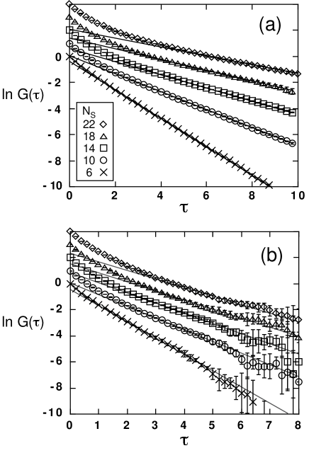
Fig.  2: Imaginary time dependence of Green functions at $\varepsilon=0$; (a) for $U=4J=2t$ and (b) for $U=4J=3t$. Note that the origin for the $y$ axis has an offset to distinguish the data for each system size in both figures. The straight lines are the fit for each data.

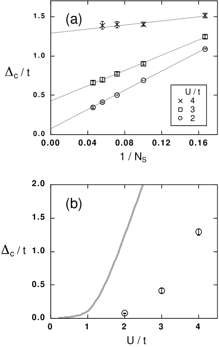
Fig.  3: QMC data for the charge gap. We fix $U/J=4$. (a) Extrapolations of the charge gap to the infinite system size. (b) The charge gap in the thermodynamic limit for various values of $U/t$ at $\varepsilon=0$. The gray curve is the result of the Hartree-Fock approximation.

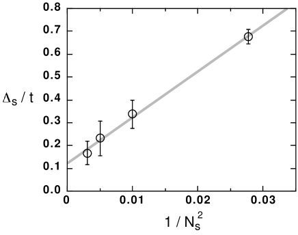
Fig.  4: QMC data for the size dependence of the spin gap at $U=4J=4t$ and $\varepsilon=0$.

Next, we discuss spin degrees of freedom. In Fig. 4, we show the QMC results of the spin gap $\Delta_{\rm S}$ calculated as the energy difference between the singlet ground state and the first triplet excitation,

$$\Delta_{\rm S}=E_{\rm g}\left(N_{\rm e}^{\uparrow}=\frac{N_{\rm e}}{2}+1;N_{\rm e}^{\downarrow}=\frac{N_{\rm e}}{2}-1\right)-E_{\rm g}\left(N_{\rm e}^{\uparrow}=\frac{N_{\rm e}}{2};N_{\rm e}^{\downarrow}=\frac{N_{\rm e}}{2}\right).$$ (55)

In the figure, we fit the data by $\Delta_{\rm S}={\rm const.}+aN_{\rm S}^{-2}$ which was used to estimate the spin gap in the $S=1$ spin system with nearest-neighbor antiferromagnetic coupling, which is often called the Haldane system .${}^{\hbox{\immediate{\bf{?}})}}$ Our data suggest a non-zero value of the spin gap in the thermodynamic limit; $\Delta_{\rm S}/t=0.12\pm 0.05$. However, our data are not accurate enough to justify this form of the fit, because of large errorbars and finite size limitation. Further investigations are necessary to estimate the spin gap $\Delta_{\rm S}$ accurately.

It should be stressed that the magnitude of the spin gap $\Delta_{\rm S}$ obtained here is much smaller than the charge gap $\Delta_{\rm C}$ plotted in Fig. 3 (b); $\Delta_{\rm S}/\Delta_{\rm C}\sim 0.1$ for $U=4J=4t$. This large discrepancy between $\Delta_{\rm C}$ and $\Delta_{\rm S}$ is characteristic for the strongly correlated insulator. Note that $\Delta_{\rm S}$ is equal to $\Delta_{\rm C}$ in the band insulator.

If we take the different values between intra- and inter-orbital Coulomb interactions, that is, $U_{11}=U_{22}>U_{12}$, an effective Hamiltonian at $\varepsilon=0$ in the limit of strong correlation is the Haldane system. As widely known, this $S=1$ spin system has been predicted to have a finite excitation gap between the singlet ground state and the triplet excited state, which is called the Haldane gap .${}^{\hbox{\immediate{\bf{?}},\penalty 1000\hskip 0.91003pt plus 0.70004pt minus 0.70004pt{\bf{?}})}}$ This conjecture has been favorably supported by both analytical ${}^{\hbox{\immediate{\bf{?}},\penalty 1000\hskip 0.91003pt plus 0.70004pt minus 0.70004pt{\bf{?}})}}$ and numerical ${}^{\hbox{\immediate{\bf{?}},\penalty 1000\hskip 0.91003pt plus 0.70004pt minus 0.70004pt{\bf{?}},\penalty 1000\hskip 0.91003pt plus 0.70004pt minus 0.70004pt{\bf{?}},\penalty 1000\hskip 0.91003pt plus 0.70004pt minus 0.70004pt{?},\penalty 1000\hskip 0.91003pt plus 0.70004pt minus 0.70004pt{\bf{?}})}}$ investigations. Our numerical result obtained above suggests that the Mott insulating state of our model at $\varepsilon=0$ may be smoothly connected with the Haldane system, that is, it may be in the same universality class in spite of finite values of $U$ and $J$, although our model with the assumption $U_{11}=U_{22}=U_{12}=U$ has an additional degeneracy in the limit of strong correlation.

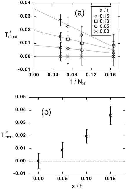
Fig.  5: QMC data of the pseudo-spin moment for $U=4J=3t$. (b) shows the values of the pseudo-spin moment as function of $\varepsilon$, which are obtained from the extrapolations to the thermodynamic limit in (a).

Finally, we consider properties in orbital degrees of freedom. In the doubly degenerate system, it is useful to describe the two orbital degrees of freedom by the pseudo-spin operator defined as

$$T_{i}^{\alpha}=\frac{1}{2}\sum_{\sigma}\sum_{\nu\nu^{\prime}}\vec{\tau}_{\nu\nu^{\prime}}^{\alpha}c_{i\nu\sigma}^{\dagger}c_{i\nu^{\prime}\sigma},$$ (56)

where $\vec{\tau}$ is the Pauli matrix and $\alpha=x$, $y$ or $z$. In order to discuss the low-lying excitations in this channel, we calculate how the pseudo-spin moment responds to its conjugate field, that is, the level split $\varepsilon$. The pseudo-spin moment is defined as

$$T_{\rm mom}^{z}=\frac{1}{N_{\rm S}}|\sum_{i}T_{i}^{z}|,$$ (57)

which signals a magnitude of self doping between two orbitals. As shown in Fig. 5 (a), the pseudo-spin moment $T_{\rm mom}^{z}$ has a finite value in the thermodynamic limit when we switch on $\varepsilon$. Fig. 5 (b) summarizes the pseudo-spin moment $T_{\rm mom}^{z}$ as function of $\varepsilon$. We find that $T_{\rm mom}^{z}$ seems to grow continuously from zero at $\varepsilon=0$, which strongly suggests a gapless nature in the orbital channel in the Mott insulating state.

4.3 Mott transition by chemical potential control

We consider here insulator-metal transitions by controlling the chemical potential $\mu$. Critical exponents are investigated from the insulating side by a technique recently proposed and applied to single-orbital Hubbard models .${}^{\hbox{\immediate{\bf{?}})}}$ In this method, the correlation length exponent $\nu$ is directly determined from the localization length $\xi_{\rm l}$ of the single-particle wave function probed by of the Green function in the long distance. Here, we explain the prescription to determine the exponent $\nu$.

Fig.  6: Imaginary time dependence of Green functions for the farthest sites at $U=4J=3t$ and $\varepsilon=0$.

Fig. 6 shows the imaginary time dependence of the Green function for the farthest sites $G(r_{ij}=N_{\rm S}/2,\tau)\equiv\sum_{\nu\sigma}G_{\nu\nu\sigma}(r_{ij}=N_{\rm S}/2,\tau)$ for each system size $N_{\rm S}$ at $\varepsilon=0$. From these data, we obtain the frequency dependent Green function for $|\mu|<\Delta_{\rm C}$ as

$$G\left(r_{ij},\omega=\mu\right)=\int_{-\infty}^{\infty}d\tau G\left(r_{ij},\tau\right)e^{\tau\mu},$$ (58)

because the density is fixed in the Mott insulating state. It should be noted that the Green function satisfies $G(r_{ij},\tau)=(-1)^{|r_{ij}|}G(r_{ij},-\tau)$ by the particle-hole symmetry. In Eq. (58), the factor $e^{\tau\omega}$ makes it difficult to estimate $G\left(r_{ij},\omega=\mu\right)$ accurately, because the statistical error with each QMC data will grow exponentially with increasing values of $\tau$ for $\tau\omega>0$. For better numerical estimation, we carry out the imaginary time integration in Eq. (58) in the following way .${}^{\hbox{\immediate{\bf{?}})}}$ Using the operator $T_{R}$ which satisfies $T_{R}^{\dagger}c_{i\nu\sigma}T_{R}=c_{i+R,\nu\sigma}$, we describe the large $\tau$ behavior of $G\left(N_{\rm S}/2,\tau\right)$ as

$$G\left(N_{\rm S}/2,\tau\right)\sim\sum_{\nu\sigma}\langle\Psi_{\rm g}^{N_{\rm e}}|T_{N_{\rm S}/2}^{\dagger}c_{i\nu\sigma}T_{N_{\rm S}/2}|\Psi_{\rm g}^{N_{\rm e}+1}\rangle\langle\Psi_{\rm g}^{N_{\rm e}+1}|c_{i\nu\sigma}^{\dagger}|\Psi_{\rm g}^{N_{\rm e}}\rangle\exp\left(-\tau\Delta_{\rm C}\right)$$ (59)

in the spectral representation as Eq. (4.2). Here, our Hamiltonian commutes with the operator $T_{N_{\rm S}/2}$ and we employ the periodic boundary conditions $T_{N_{\rm S}/2}^{2}=1$. Therefore, $G\left(N_{\rm S}/2,\tau\right)\sim\pm G\left(\tau\right)$ for large $\tau$, because $T_{N_{\rm S}/2}|\Psi_{\rm g}^{N_{\rm e}}\rangle=\pm|\Psi_{\rm g}^{N_{\rm e}}\rangle$. Here $G(\tau)$ is the uniform Green function defined in Eq. (54). With this property, we estimate the integration in Eq. (58) by substituting the large $\tau$ behavior of $G\left(\tau\right)$, that is, $\alpha\exp\left(-\tau\Delta_{\rm C}\right)$, for that of $G\left(N_{\rm S}/2,\tau\right)$, as

$$|G\left(r_{ij},\omega=\mu\right)|=\int_{-\tau_{0}}^{+\tau_{0}}d\tau|G\left(N_{\rm S}/2,\tau\right)|e^{\tau\mu}+\alpha\left[\int_{+\tau_{0}}^{+\infty}e^{\tau\left(\mu-\Delta_{\rm C}\right)}+\int_{-\infty}^{-\tau_{0}}e^{\tau\left(\mu+\Delta_{\rm C}\right)}\right].$$ (60)

Here, we take the threshold value $\tau_{0}$ such that for $\tau>\tau_{0}$ the tail of $G\left(N_{\rm S}/2,\tau\right)$ obeys $\alpha\exp\left(-\tau\Delta_{\rm C}\right)$ within our numerical accuracy. The advantage in Eq. (60) lies in the fact that $G\left(\tau\right)$ generally shows better numerical convergence for large $\tau$ than $G\left(N_{\rm S}/2,\tau\right)$.

Fig. 7 (a) represents $N_{\rm S}$ dependence of $G(N_{\rm S}/2,\omega=\mu)$ at $\varepsilon=0$ for various values of the chemical potential $\mu$ obtained by the above prescription. For each value of $\mu$, $G\left(N_{\rm S}/2,\mu\right)$ decays exponentially with $N_{\rm S}$ due to a finite localization length $\xi_{\rm l}$ in the insulating state, that is, $G(r_{ij},\mu)\sim\exp(-|r_{ij}|/\xi_{\rm l})$. We determine the localization length $\xi_{\rm l}$ from the decay rates in Fig. 7 (a). Fig. 7 (b) gives a log-log plot between $\xi_{\rm l}$ and $|\mu-\Delta_{\rm C}|$, which determines the critical exponent $\nu$ directly through a scaling relation

$$\xi_{\rm l}\sim|\mu-\Delta_{\rm C}|^{-\nu}.$$ (61)

We note that the charge gap is determined from Eq. (52) independently of this procedure. In this case with $\varepsilon=0$, the QMC data may be consistently understood by $\nu=1/2$. We will discuss this result as well as the scaling relation Eq. (61) in Sec. 5.1.

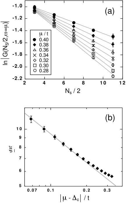
Fig.  7: Schemes to calculate the localization length $\xi_{\rm l}$ and the correlation length exponent $\nu$. See text for details. (a) Distance dependence of the Green function for various values of the chemical potential $\mu$. (b) Algebraic divergence of the localization length toward the critical point. The gray line corresponds to $\xi_{\rm l}\sim|\mu-\Delta_{\rm C}|^{-1/2}$.

4.4 Self doping by level split control

In this section, we concentrate on the control of the level split $\varepsilon$. When we change the level split $\varepsilon$, the self doping between two orbitals occurs continuously from $\varepsilon=0$, because of the gapless nature in pseudo-spin degrees of freedom discussed in Sec. 4.2.

Fig. 8 shows the typical behaviors of the momentum distribution function defined as

$$n_{\nu}\left(k\right)=\frac{1}{N_{\rm S}}\sum_{ij\sigma}\langle c_{i\nu\sigma}^{\dagger}c_{j\nu\sigma}\rangle e^{{\rm i}kr_{ij}}.$$ (62)

At $\varepsilon=0$, $n_{\nu=1}(k)$ is equal to $n_{\nu=2}(k)$ because of the symmetry about the orbital index, and the characteristic wave number $k^{*}$ where $n_{1}(k)$ has the largest slope is at $\pi/2$. When $\varepsilon$ becomes larger, the form of $n_{1}(k)$ changes continuously and the wave number $k^{*}$ approaches zero. Note that the relation $n_{2}(k)=1-n_{1}(\pi-k)$ holds for all the values of $\varepsilon$ by the particle-hole symmetry. The area under the curve of $n_{\nu}(k)$ corresponds to the density in the orbital $\nu$, therefore these behaviors of the momentum distribution function clearly represent the self doping from the orbital $\nu=1$ to $\nu=2$.

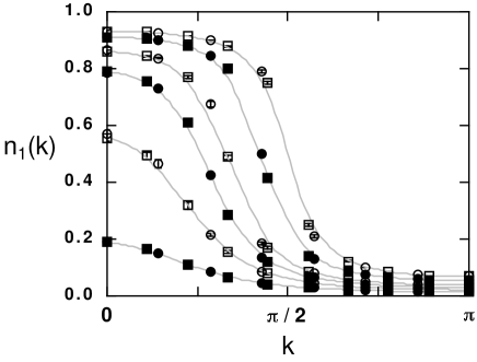
Fig.  8: Momentum distribution functions of the orbital $\nu=1$ for the level split control at $U=4J=3t$. The gray curves are guides to eye. The data are for $\varepsilon/t=0.0,0.4,0.8,1.0,1.2$ and $1.4$ from the top to the bottom. The circles and squares correspond to the data for $N_{\rm S}=14$ and $18$, respectively.

Fig. 9 shows the $\varepsilon$ dependence of the pseudo-spin moment defined in Eq. (57). As shown in Fig. 9 (a), the pseudo-spin moment $T_{\rm mom}^{z}$ grows continuously from zero at $\varepsilon=0$ and approaches $1$ for large values of $\varepsilon$. The behavior of $T_{\rm mom}^{z}$ for large $\varepsilon$ is also plotted in Fig. 9 (b) as function of $\varepsilon^{-1}$. This asymptotic behavior of the magnitude of the self doping is discussed in Sec. 5.2.

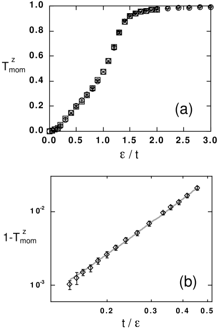
Fig.  9: Pseudo-spin moment for the level split control at $U=4J=3t$. The asymptotic behavior of the self doping for large values of $\varepsilon$ is illustrated in (b). The gray curve is the fit by $a/\varepsilon^{2}+b/\varepsilon^{3}$. In both figures, the diamonds, circles and squares correspond to the data for $N_{\rm S}=10$, $14$ and $18$, respectively.

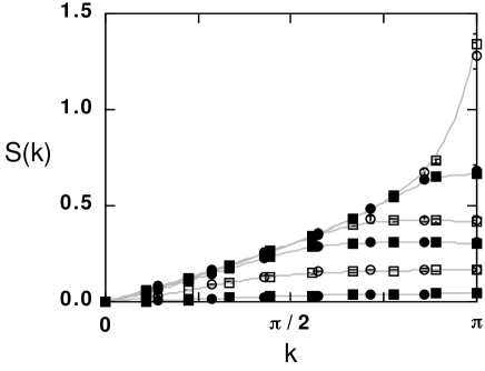
Fig.  10: Spin correlation functions for the level split control at $U=4J=3t$. The gray curves are guides to eye. The data are for $\varepsilon/t=0.0,0.4,0.8,1.0,1.2$ and $1.4$ from the top to the bottom. The circles and squares correspond to the data for $N_{\rm S}=14$ and $18$, respectively.

Fig.  11: The antiferromagnetic spin correlation as function of the pseudo-spin moment at $U=4J=3t$. The inset shows the behavior of the inverse of $S(\pi)$ near $T_{\rm mom}^{z}=0$. The circles and squares correspond to the data for $N_{\rm S}=14$ and $18$, respectively.

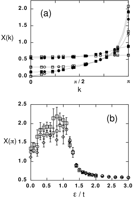
Fig.  12: (a) Anomalous correlation functions for the level split control at $U=4J=3t$. The gray curves are guides to eye. The data are for $\varepsilon/t=0.0,0.6,1.0,1.4$ and $2.0$ from the bottom to the top at $k=0$. (b) $\varepsilon$ dependence of $X(\pi)$. In both figures, the diamonds, circles and squares correspond to the data for $N_{\rm S}=10,14$ and $18$, respectively.

The spin correlation functions for various values of $\varepsilon$ are shown in Fig. 10. The definition of the spin correlation function is

$$S\left(k\right)=\frac{1}{N_{\rm S}}\sum_{ij}\langle S_{i}S_{j}\rangle e^{{\rm i}kr_{ij}},$$ (63)

where $S_{i}=\left(S_{i}^{x}+S_{i}^{y}+S_{i}^{z}\right)/3$. The spin operator is defined as

$$S_{i}^{\alpha}=\frac{1}{2}\sum_{\nu}\sum_{\sigma\sigma^{\prime}}\vec{\tau}_{\sigma\sigma^{\prime}}^{\alpha}c_{i\nu\sigma}^{\dagger}c_{i\nu\sigma^{\prime}}$$ (64)

with the Pauli matrix $\vec{\tau}$ and $\alpha=x$, $y$ or $z$. At $\varepsilon=0$, although it has a spin excitation gap as examined in Sec. 4.2, $S(k)$ has a large peak at $k=\pi$ originating from the short-range antiferromagnetic correlation in the Mott insulator. When we change the level split $\varepsilon$, this structure collapses and the peak is broadened continuously.

In Fig. 11, we summarize the values of the antiferromagnetic correlation $S(\pi)$ as function of the pseudo-spin moment $T_{\rm mom}^{z}$ which corresponds to the magnitude of self doping. The inset of Fig. 11 plots the inverse of $S(\pi)$ in the small self-doped region. These behaviors of the spin correlation for the self doping are discussed in Sec. 5.2.

As mentioned in Sec. 2.5, for a finite value of $\varepsilon$, the nesting property between different orbitals may play a significant role. Actually, in the mean-field analysis which is discussed in Appendix C, the system keeps the insulating nature when we change $\varepsilon$ from zero, where the energy gap opens by the order parameter which corresponds to the scattering process between different spins and orbitals. This relevant process is represented by the operator

$$X_{i}=\frac{1}{2}\sum_{\nu\nu^{\prime}}\sum_{\sigma\sigma^{\prime}}\vec{\tau}_{\nu\nu^{\prime}}^{x}\vec{\tau}_{\sigma\sigma^{\prime}}^{x}c_{i\nu\sigma}^{\dagger}c_{i\nu^{\prime}\sigma^{\prime}}.$$ (65)

The correlation function of this operator, $X(k)$, is defined as

$$X\left(k\right)=\frac{1}{N_{\rm S}}\sum_{ij}\langle X_{i}X_{j}\rangle e^{{\rm i}kr_{ij}}.$$ (66)

We call this the anomalous correlation function.

In Fig. 12 (a), we show the behaviors of the anomalous correlation function $X(k)$ with the change of the level split $\varepsilon$. Note that in the non-interacting case, $X(k)$ takes the constant value $1/2$ by definition. We plot the values of $X(\pi)$ in Fig. 12 (b). Compared with the monotonic decrease of the spin correlation $S(\pi)$, $X(\pi)$ is enhanced for small values of $\varepsilon$ and keeps almost constant values up to $\varepsilon\sim t$. This behavior is discussed in Sec. 5.2 in comparison with the mean-field results obtained in Appendix C.

5 Discussion

In this section, we discuss the numerical results in one dimension obtained in the previous section. The Mott transition by the chemical potential control is analyzed based on the scaling theory. The behaviors by changing the level split are discussed as the crossover between the Mott insulator with high spin state and the band insulator with low spin state. The relevance of our results to experimental situations is also remarked. We also compare our results with previous theoretical investigations.

5.1 Hyperscaling analysis

In this part, the QMC data for the insulator-metal transitions controlled by the chemical potential obtained in Sec. 4.3 are analyzed based on the hyperscaling hypothesis. The universality class is examined by combining scaling relations with the QMC results.

Note that the hyperscaling analysis assumes the continuous transition. All the numerical data in our investigations do not show any apparent discontinuity expected in first-order transitions. This implies that the transitions are always continuous here, although we can not exclude the possibility of a weak first-order transition with small discontinuity. In this section, we assume the continuous transitions and employ the hyperscaling hypothesis.

First, we briefly review scaling arguments for continuous metal-insulator transitions .${}^{\hbox{\immediate{\bf{?}},\penalty 1000\hskip 0.91003pt plus 0.70004pt minus 0.70004pt{\bf{?}},\penalty 1000\hskip 0.91003pt plus 0.70004pt minus 0.70004pt{\bf{?}})}}$ The hyperscaling hypothesis asserts that a single characteristic length scale $\xi$ and a single energy scale $\Omega$ govern the quantum critical phenomena. The scaling behaviors of these two quantities give two basic critical exponents; the correlation length exponent $\nu$ and the dynamical exponent $z$, as

$$\xi \sim |\Delta|^{-\nu}$$ (67)

$$\Omega \sim \xi^{-z}\sim|\Delta|^{z\nu},$$ (68)

where $\Delta$ is a control parameter for the transition which measures a distance from the critical point. With these two exponents $\nu$ and $z$, the finite-size scaling for the singular part of the free energy density in $d$ dimensions is given by

$$f_{\rm S}\left(\Delta\right)\sim\Delta^{\nu\left(d+z\right)}F\left(\xi/L,\xi^{z}/\beta\right),$$ (69)

where $F$ is a finite-size scaling function, $L$ is a linear dimension of the system and $\beta$ is the inverse temperature. Comparing differentiations of $f_{\rm S}$ by $L$ or $\beta$ with the Taylor expansion of the free energy density for twists of spatial or temporal boundary conditions with dimensional analysis, we obtain the scaling behaviors for the singular part of physical quantities; for example,

charge susceptibility $$: \quad\kappa\sim\Delta^{-\nu\left(z-d\right)}$$ (70)

localization length $$: \quad\xi_{\rm l}\sim\Delta^{-\nu}.$$ (71)

The last one Eq. (71) is the same as Eq. (61).

It is important to notice that the charge susceptibility $\kappa$ can also be deduced directly from the definition $-\partial^{2}f/\partial\Delta^{2}$ where $\Delta$ expresses the chemical potential $\mu$. Direct differentiation of Eq. (69) gives

$$\kappa\sim\Delta^{\nu\left(d+z\right)-2}.$$ (72)

If we compare this relation with Eq. (70), we obtain an important relation

$$z\nu=1$$ (73)

for metal-insulator transitions by the chemical potential.

In Sec. 4.3, we studied the correlation length exponent $\nu$ directly from the insulating side. The QMC data of the localization length $\xi_{\rm l}$ in Fig. 7 (b) suggests $\nu=1/2$.

The criticality of the filling-control Mott transitions itself in one dimension has been investigated based on the scaling theory .${}^{\hbox{\immediate{?})}}$ There, the critical nature has been discussed depending on whether component (spin or orbital) orderings exist or not both in insulators and in metals. The prediction of these scaling arguments is that all the Mott transitions by controlling the chemical potential in one dimension should be characterized by $\nu=1/z=1/2$. Our result, $\nu=1/2$ for the doubly degenerate Hubbard model also support at least this estimate for $\nu$ and hence it is plausible that it satisfies the hyperscaling with $\nu=1/z=1/2$.

5.2 Effect of self doping

Here, we discuss the effects of the level split based on the numerical results obtained in Sec. 4.4. In this one-dimensional system, our results indicate the crossover between the Mott insulator with high spin state and the band insulator with low spin state with the self doping by the level split.

At $\varepsilon=0$, the system is in the Mott insulating state. As discussed in Sec. 4.2, this state has a finite spin gap and a gapless excitation in the orbital channel. In this state, two spins in degenerate orbitals couple with each other ferromagnetically by the Hund coupling, that is, they form the $S=1$ high spin state. These $S=1$ spins show the short-range antiferromagnetic correlation which leads to the peak structure of the spin correlation function as shown in Fig. 10.

On the other hand, in the limit $\varepsilon\gg U,J$ and $t$, the system should behave as the band insulator. Note that for $\varepsilon>2t$, the system becomes an insulator even in the non-interacting case. In this limit, two orbitals are split by large $\varepsilon$ and particles predominantly occupy the one orbital $\nu=2$. This behavior is clearly seen in Fig. 9 (a). For large values of $\varepsilon$, a small density in the orbital $\nu=1$ may be induced by the ${\cal H}_{J}$ term Eq. (51). By the perturbation in $1/\varepsilon$, the energy gain from this mixing is the order of $-J^{2}/2\varepsilon$. The fraction of the density in the orbital $\nu=1$ is estimated by the $\varepsilon$ derivative of this gain, therefore its leading term should be $O(\varepsilon^{-2})$. As shown in Fig. 9 (b), the QMC data of $1-T_{\rm mom}^{z}$ for large $\varepsilon$ are well fitted by $a\varepsilon^{-2}+b\varepsilon^{-3}$. If we assume the rigid-band picture, the energy split between highest-occupied and lowest-unoccupied states is given by $2\varepsilon-W^{*}$ with the bandwidth $W^{*}$ renormalized by the interactions. Then the $\varepsilon$ derivative of $-J^{2}/(2\varepsilon-W^{*})$ results in $1-T_{\rm mom}^{z}\simeq\frac{J^{2}}{2\varepsilon^{2}}\left(1+W^{*}/\varepsilon\right)$, therefore, the ratio $b/a=W^{*}$. From the fit in Fig. 9 (b), we obtain $W^{*}/t=3.6\pm 0.3$. This indicates the bandwidth is narrowed by the interactions compared with the non-interacting bandwidth $4t$ in this rigid-band scheme. In the spin sector, in this band-insulator limit, the spin moment is close to zero, that is, the low spin state is realized. This feature is clearly seen in the flat structure of the spin correlation in Fig. 10.

Between these two limiting behaviors, our QMC results obtained in Sec. 4.4 suggest the crossover from one to the other. Both the pseudo-spin moment and the spin correlation change continuously by the level split, as shown in Figs. 9 and 10. In the region $\varepsilon\mathrel{\mathchoice{\lower 2.5pt\vbox{\halign{$\m@th\displaystyle\hfil#\hfil$\cr<\crcr\sim\crcr}}}{\lower 2.5pt\vbox{\halign{$\m@th\textstyle\hfil#\hfil$\cr<\crcr\sim\crcr}}}{\lower 2.5pt\vbox{\halign{$\m@th\scriptstyle\hfil#\hfil$\cr<\crcr\sim\crcr}}}{\lower 2.5pt\vbox{\halign{$\m@th\scriptscriptstyle\hfil#\hfil$\cr<\crcr\sim\crcr}}}}t$, as shown in Fig. 12, the anomalous correlation defined in Eq. (66) has a peak structure at $k=\pi$. This indicates that the Umklapp process between different spins and orbitals is relevant to the insulating nature in this region. In the mean-field calculations, the importance of this process is also pointed out as discussed in Appendix C. Of course, the mean-field description is known to break down for one-dimensional systems: It predicts the long-range order of this correlation and the phase transition between the Mott insulator and the band insulator as shown in Fig. 17.

When the degenerate orbitals split up by increasing the value of $\varepsilon$, our numerical results show that the spin correlation is sensitive to a small self doping. As shown in Fig. 11, for $U=4J=3t$, only $15\%$ self doping is enough to reduce the value of $S(\pi)$ to the half of that at $\varepsilon=0$. For spin systems with a finite spin gap, the spin correlation function has a Lorentzian-type peak at $k=\pi$ as

$$S(k)\propto\left[\left(k-\pi\right)^{2}+\xi_{\rm S}^{-2}\right]^{-1/2},$$ (74)

where $\xi_{\rm S}$ is the spin correlation length. This spin correlation length determines the spin gap; $\Delta_{\rm S}\sim\xi_{\rm S}^{-1}$. Although this form of $S(k)$ is not rigorously applicable to the case for $\varepsilon\neq 0$, it should be reasonable to consider that the peak value of $S(k)$ at $k=\pi$ may be related to the spin correlation length as well as the spin gap at least for $\varepsilon\ll U$. The rapid decay of $S(\pi)$ against the self doping in Fig. 11 suggests the rapid growth of the spin gap from the value in the Mott insulator at $\varepsilon=0$. The inset of Fig. 11 indicates that the spin gap increases linearly with increasing the magnitude of self doping.

5.3 Comparison with other experimental and theoretical studies

In Sec. 5.1, the universality class characterized by $\nu=1/z=1/2$ is suggested for the Mott transitions controlled by the chemical potential of the doubly degenerate Hubbard model in one dimension. This result is considered to be relevant to the metal-insulator transitions when mobile holes are introduced into the one-dimensional strongly correlated insulator with a finite spin gap; the $S=1$ Haldane system, the spin-Peierls system or the spin ladder system with even-number legs.

Experimentally, the hole doping to the spin-gap material has been realized in (Y,Ca)₂BaNiO₅ .${}^{\hbox{\immediate{\bf{?}},\penalty 1000\hskip 0.91003pt plus 0.70004pt minus 0.70004pt{\bf{?}})}}$ The material Y₂BaNiO₅ is a typical Haldane system with the spin gap $\sim 100K$ ,${}^{\hbox{\immediate{?},\penalty 1000\hskip 0.91003pt plus 0.70004pt minus 0.70004pt{?})}}$ where two spins in the $e_{g}$ orbital in the $d^{8}$ configuration of Ni²⁺ construct the one-dimensional network as mentioned in Sec. 3.2. When we replace Y³⁺ with Ca²⁺ partially, the charge doping into this chain is realized. Unfortunately, in this system, the doped holes did not show a clean metallic behavior, although the density of states within the Haldane gap is induced by them .${}^{\hbox{\immediate{?})}}$ The temperature dependence of the magnetic susceptibility shows a spin-glass like history at low temperature .${}^{\hbox{\immediate{?})}}$ These experimental results indicate that introduced holes are localized by some disorder. For the direct comparison with our result, a material showing the metallic behavior with hole doping is desired. Effects of disorder on our theoretical result also remains for further study for comparison with the available experimental results.

Theoretically, several one-dimensional models have been known to have a finite spin excitation gap in the Mott insulating state; for example, the $t$-$J$-$J^{\prime}$ model ,${}^{\hbox{\immediate{\bf{?}})}}$ the dimerized $t$-$J$ model ,${}^{\hbox{\immediate{\bf{?}})}}$ the $t$-$J$ ladder model with even-number legs .${}^{\hbox{\immediate{\bf{?}},\penalty 1000\hskip 0.91003pt plus 0.70004pt minus 0.70004pt{\bf{?}},\penalty 1000\hskip 0.91003pt plus 0.70004pt minus 0.70004pt{\bf{?}},\penalty 1000\hskip 0.91003pt plus 0.70004pt minus 0.70004pt{\bf{?}})}}$ These models have been investigated with emphasis on the possible persistence of the spin gap in the metallic phase and on a realization of the superconductivity near the Mott insulator. From this point of view, the metallic region away from half filling in our model provides another interesting example along this line. However, in our model, another potential candidate of metals is a ferromagnetic phase due to the double exchange mechanism. In this work, we have not investigated this problem mainly because of the negative sign difficulty in numerical calculations as discussed in Appendix B. This interesting problem remains for further study.

Next, we give remarks on the experimental relevance of the crossover behavior indicated in Sec. 5.2. As discussed in Sec. 3.2, there are several one-dimensional systems which are often called the Haldane materials. In these systems, the one-dimensional structure itself may induce the deformation of the surrounding ligands, which leads to the level split between two orbitals in the $e_{g}$ state. The magnitude of this level split is difficult to estimate experimentally in general. However, it can be the same order as the bandwidth or the Hund coupling. Our results suggest that if this happens, the analysis based on the theoretical results for the Heisenberg Hamiltonian may not work straightforwardly because of the gapless nature of orbital degrees of freedom as is discussed in Sec. 4.2. For the finite level split, it is not clear whether the effective spin Hamiltonian justified in the strong coupling limit is applicable. Our result implies the necessity to start from the tight-binding Hamiltonian as we discussed in this paper at least for quantitative analysis.

In Sec. 5.2, the linear increase of the spin gap with increase of the self doping is discussed. As mentioned in Sec. 3.2, the self doping may be induced by the change of the ligand field, which is caused also by external pressure. Recently, the Haldane material Ni(C₂H₈N₈)₂NO₂(ClO₄) (NENP) has been investigated under the external pressure .${}^{\hbox{\immediate{\bf{?}})}}$ It shows that the spin gap grows linearly with the pressure. Since the pressure does not only simply increase the level split or the self doping but also the hopping matrix, that is, the bandwidth, we need a care in analyzing it. However, our result on the effect of self doping gives at least one promising explanation for the origin for the pressure dependence of the spin gap.

6 Summary

In this work, the multi-orbital Hubbard models are investigated by the unbiased technique, the auxiliary field QMC method. The general framework of the numerical method is introduced for the multi-orbital models in detail. This technique is applicable for arbitrary number of orbitals in arbitrary dimension. We present explicitly that there exist the non-trivial cases where the negative sign problem is absent. Using this new technique, the one-dimensional models with doubly degenerate orbitals have been investigated in the ground state. Some of basic properties of the Mott insulator at half filling are quantitatively clarified. The charge and spin gap amplitudes are calculated and the characteristic behavior of them as the strongly correlated insulator is clarified. The charge gap can be one order of magnitude larger than the spin gap in our result of the Mott insulating phase. The orbital degrees of freedom are shown to have a gapless excitation. By controlling the chemical potential, the critical properties of the insulator-metal transition have been investigated. We obtain the correlation length exponent $\nu=1/2$ which is consistent with the general prediction by the scaling arguments. The universality class for this transition has been discussed by analyzing our numerical results based on the hyperscaling hypothesis. For the level split between two orbitals, the effect of self doping is examined in detail. Our numerical results of correlation functions indicate the crossover between the Mott insulator with high spin state and the band insulator with low spin state. The significance of the Umklapp scattering between different spins and orbitals in this crossover is suggested. With increase of the level split, remarkably different spin and charge gap amplitudes in the Mott insulating phase continuously crossover to a similar value in the band insulating phase. The antiferromagnetic spin correlation as well as the inverse of the spin gap sensitively decreases with the self doping. Our result of the chemical potential control may have relevance to the hole doping of the Haldane materials. Our result of the rapid increase of the spin gap by the self doping is consistent with the experimentally observed increase of the spin gap in the Haldane materials under pressure.

Appendix A

In this part, numerical convergence in the actual QMC calculations is examined in detail. As described in Sec. 2, in the auxiliary field algorithm for the ground state, we should take care of the convergence about two quantities; one is the width of the Suzuki-Trotter slice $\Delta\tau$ and the other is the magnitude of the projection $\beta$. We discuss the behavior of these systematic errors for the doubly degenerate model defined in Sec. 3.1.

First, we examine the convergence about $\Delta\tau$. As discussed in Sec. 2, the systematic errors dominantly come from the Suzuki-Trotter decomposition Eq. (9). The magnitude of the error depends on the parameters in the Hamiltonian as well as on the physical quantities which we measure. Fig. 13 shows the $\Delta\tau$ dependence of the ground state energy per site and orbital, $\varepsilon_{\rm g}\equiv E_{\rm g}/2N_{\rm S}$, for two sets of parameters, (a) $U=4J=2t$ and (b) $U=4J=3t$. The data are for $14$-site systems with $\varepsilon=0$. Among the quantities which we have calculated, the ground state energy has the strongest dependence on $\Delta\tau$. As shown in Fig. 13, the QMC data are well fitted by

$$\varepsilon_{\rm g}=\varepsilon_{\rm g}^{\rm ext}-a\left(\Delta\tau\right)^{2},$$ (75)

as expected from the decomposition Eq. (9). Here $\varepsilon_{\rm g}^{\rm ext}$ denotes the extrapolated value to the limit $\Delta\tau\rightarrow 0$, which is plotted as the diamonds in Fig. 13. In actual QMC calculations, instead of obtaining $\varepsilon_{\rm g}^{\rm ext}$ by this extrapolation, we take small $\Delta\tau$ enough to guarantee the convergence within numerical errorbars for each interaction parameters. For example, we employ $\Delta\tau t=0.05$ for $U=4J=2t$ and $\Delta\tau t=0.04$ for $U=4J=3t$. From Fig. 13, these values of $\Delta\tau$ are found to ensure the numerical convergence to the limit $\Delta\tau\rightarrow 0$.

Next, the convergence about the projection $\beta$ is discussed. In general, the ground state should be projected out from a trial state for large $\beta$ compared with the inverse of the smallest energy scale in the system. Therefore, the values of $\beta$ sufficient to obtain converged data strongly depend on the model parameters as well as the trial state. We illustrate this behavior for the change of the level split $\varepsilon$. Fig. 14 shows the $\beta$ dependence of the pseudo-spin moment defined in Eq. (57) for various values of $\varepsilon$. Deviations from the converged values are plotted in the figures. In actual calculations, we check the convergence for each parameter and physical quantity carefully, and obtain the results by averaging several data for different values of $\beta$ in the converged region.

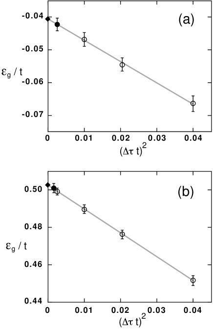
Fig.  13: $\Delta\tau$ dependence of the QMC data for the ground state energy of the doubly degenerate Hubbard model. The data are for $14$-site systems with $\varepsilon=0$; (a) $U=4J=2t$ and (b) $U=4J=3t$. Extrapolated values to $\Delta\tau\rightarrow 0$ by the fit shown as the gray lines are plotted by the diamonds. Filled circles are the data for the values of $\Delta\tau$ which we employ in the actual calculations. See text for details.

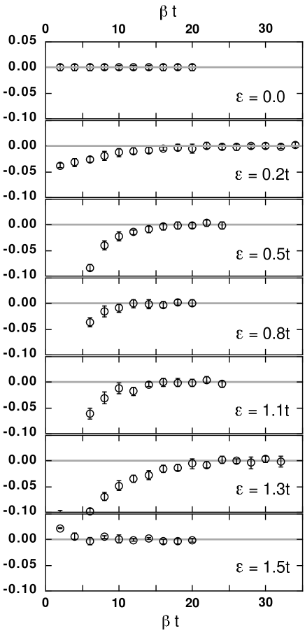
Fig.  14: $\beta$ dependence of the QMC data for the pseudo-spin moment of doubly degenerate Hubbard model for various values of the level split. The data are for $14$ site systems with $U=4J=3t$. Differences from the converged values which we determine are plotted.

Appendix B

Here we discuss the behavior of the negative sign in our framework introduced in Sec. 2. Especially, we focus two different elements which break the particle-hole symmetry and lead to the negative sign problem; the long-range hopping and the hole or electron doping.

First, we examine the effect of the long-range hopping. We add the next-nearest neighbor hopping proportional to $t^{\prime}$ to the doubly degenerate model Eqs. (48) $\sim$ (51). Note that this term is different from the next-nearest neighbor hopping term discussed in Sec. 2.5; here we consider $t_{\langle\langle ij\rangle\rangle}^{11}=t_{\langle\langle ij\rangle\rangle}^{22}=t^{\prime}\geq 0$. Fig. 15 shows the behavior of the negative sign when we change the value of $t^{\prime}$ at half filling. The negative sign $\langle S\rangle$ is defined as the real part of the phase of MC weights,

$$\langle S\rangle={\cal R}\!{\sl e}\,\frac{\langle W_{\uparrow}W_{\downarrow}\rangle}{\langle|W_{\uparrow}W_{\downarrow}|\rangle}.$$ (76)

Next, the effect of the hole doping is discussed. Fig. 16 plots the values of $\langle S\rangle$ when we introduce the extra holes or electrons to the model Eqs. (48) $\sim$ (51) at half filling. We choose the electron filling which is closed-shell configuration. As shown in Fig. 16, the negative sign difficulty is far severe in this case as compared with the results in Fig. 15. This may be partly because our HS transformation Eq. (2.2) contains the total density as the phase factor; The change of the electron filling seems to be crucial to break the phase coherence of each MC samples which is maintained at half filling.

Fig.  15: $\beta$ dependence of the negative sign for the change of the next-nearest neighbor hopping in $10$ site systems with $U=4J=2t$. The dashed lines are guides to eyes. The data are for $t^{\prime}/t=0.2,0.4,0.6,0.8$ and $1.0$ from the top to the bottom.

Fig.  16: $\beta$ dependence of the negative sign for the hole doping. The filled circles are for $N_{\rm S}=6$ and $N_{\rm e}=20$. The open diamonds are for $N_{\rm S}=10$ and $N_{\rm e}=12$.

Appendix C

In this Appendix, by using the mean-field approximation, we discuss overall features of phase diagrams for the doubly degenerate Hubbard model defined in Eqs. (48) $\sim$ (51). In Sec. 4, the QMC calculations are done for one-dimensional systems. It is difficult to compare the mean-field results with the QMC results directly, because strong quantum fluctuations in one dimension lead to the breakdown of the mean-field approach. Nevertheless, the mean-field picture is useful to understand the basic properties of the model.

For the chemical potential control, the mean-field phase diagram for the doubly degenerate Hubbard model has been investigated by Inagaki and Kubo in three dimensions .${}^{\hbox{\immediate{?})}}$ They have especially concentrated on various spin and orbital states. We discuss here their results near half filling which are the issue of our investigation in Sec. 4 and 5. For $\varepsilon=0$, at half filling, the system becomes an insulator with spin antiferromagnetic long-range order and no orbital ordering for infinitesimal Coulomb interaction. When we change the chemical potential $\mu$, the insulator-metal transition occurs and the metallic state with the antiferromagnetic ordering appears. For further change of $\mu$, this spin ordering disappears and the metal without any ordering of spin and orbital components is realized. All these features are common to the mean-field phase diagram for the single-orbital Hubbard model .${}^{\hbox{\immediate{\bf{?}})}}$

For the change of the level split $\varepsilon$, we obtain the Hartree-Fock phase diagrams following the method by Inagaki and Kubo .${}^{\hbox{\immediate{?})}}$ Here we fix the interaction ratio $U/J=4$. Our Hartree-Fock calculations are done in one dimension.

Fig. 17 (a) shows the mean-field phase diagram in the plane of the level split $\varepsilon$ and the interaction strength $U$. At $\varepsilon=0$, the antiferromagnetic insulator appears for $U>0$ as mentioned above. In this state, the antiferromagnetic order parameter $\langle c_{k\nu\uparrow}^{\dagger}c_{k+\pi\nu\downarrow}\rangle$ has the same value as $\langle c_{k\nu\uparrow}^{\dagger}c_{k+\pi\nu^{\prime}\downarrow}\rangle$ because of the symmetry about the orbital index $\nu$ at $\varepsilon=0$. When we switch on $\varepsilon$, the latter $\langle c_{k\nu\uparrow}^{\dagger}c_{k+\pi\nu^{\prime}\downarrow}\rangle$ survives and the self doping begins as shown in Fig. 17 (b). There, the insulating state persists for $\varepsilon\neq 0$ presumably because of the nesting properties between different spins and orbitals as discussed in the last part of Sec. 2. The self doping occurs continuously until all the electrons occupy the orbital $\nu=2$, that is, the phase transition to the band insulating state. The mean-field results for the charge gap $\Delta_{\rm C}$ which is defined in Eq. (52) are plotted in Fig. 17 (c). The charge gap has a finite value for all the values of $\varepsilon$. However, the origin of the gap is clearly different between two phases in Fig. 17 (a). For small values of $\varepsilon$, the gap originates from the nesting properties and the ordering of $\langle c_{k\nu\uparrow}^{\dagger}c_{k+\pi\nu^{\prime}\downarrow}\rangle$, and the value of the gap decreases gradually. Compared to this, for large values of $\varepsilon$, the gap increases linearly as the function of $\varepsilon$, which is expected for the band insulating state.

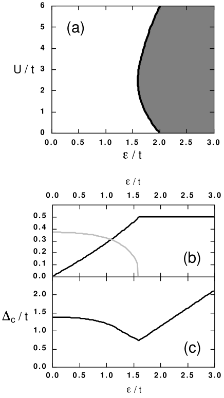
Fig.  17: Mean-field results for the level split control; (a) Phase diagram. We fix $U=4J$. The gray area represents a band insulator. The white area shows an insulating state due to the nesting properties between different spins and orbitals. (b) The mean fields as function of $\varepsilon$ at $U=4J=2t$. The black curve denotes $(-1)^{\nu}\left(\langle n_{i\nu\sigma}\rangle-1/2\right)=\langle T_{\rm mom}^{z}\rangle/2$, which corresponds to the magnitude of the self doping. The gray one is for $\langle c_{k\nu\sigma}^{\dagger}c_{k+\pi,\nu^{\prime}\sigma^{\prime}}\rangle$. (c) $\varepsilon$ dependence of the charge gap at $U=4J=2t$.

References

- [1] J. G. Bednort and K. A. Müller: Z. Phys. B 64 (1986) 189.
- [2] For a review for electron systems, see M. Imada, A. Fujimori and Y. Tokura: Rev. Mod. Phys. 70 (1998) No.3.
- [3] B. H. Brandow: Adv. Phys. 26 (1977) 651.
- [4] J. Kanamori: Prog. Theor. Phys. 30 (1963) 275.
- [5] L. M. Roth: Phys. Rev. 149 (1966) 306.
- [6] L. M. Roth: J. Appl. Phys. 38 (1967) 1065.
- [7] K. I. Kugel’ and D. I. Khomskiĭ: Sov. Phys. Ups. 25 (1982) 231.
- [8] K. I. Kugel’ and D. I. Khomskiĭ: Sov. Phys. JETP. 37 (1973) 725.
- [9] S. Inagaki and R. Kubo: Int. J. Mag. 4 (1973) 139.
- [10] M. Cyrot and C. Lyon-Caen: J. Phys. Paris 36 (1975) 253.
- [11] J. Bünemann and W. Weber: Phys. Rev. B 55 (1997) 4011.
- [12] T. Okabe: J. Phys. Soc. Jpn. 66 (1997) 2129.
- [13] T. Okabe: J. Phys. Soc. Jpn. 65 (1996) 1056.
- [14] K. A. Chao and M. C. Gutzwiller: J. Appl. Phys. 42 (1971) 1420.
- [15] K. A. Chao: Phys. Rev. B 4 (1971) 4034.
- [16] J. P. Lu: Phys. Rev. B 49 (1994) 5687.
- [17] G. Kotliar and H. Kajueter: Phys. Rev. B 54 (1996) 14221.
- [18] M. J. Rozenberg: Phys. Rev. B 55 (1997) 4855.
- [19] H. Hasegawa: J. Phys. Soc. Jpn. 66 (1997) 1391.
- [20] H. Hasegawa: Phys. Rev. B 56 (1997) 1196.
- [21] H. Hasegawa: J. Phys. Soc. Jpn. 66 (1997) 3522.
- [22] Y. Motome and M. Imada: J. Phys. Soc. Jpn. 66 (1997) 1872.
- [23] J. E. Hirsch: Phys. Rev. B 28 (1983) 4059.
- [24] J. E. Hirsch: Phys. Rev. B 31 (1985) 4403.
- [25] G. Sugiyama and S. E. Koonin: Annals of Phys. 168 (1986) 1.
- [26] S. R. White, D. J. Scalapino, R. L. Sugar, E. Y. Loh, J. E. Gubernatis and R. T. Scalettar: Phys. Rev. B 40 (1989) 506.
- [27] M. Imada and Y. Hatsugai: J. Phys. Soc. Jpn. 58 (1989) 3752.
- [28] H. F. Trotter: Proc. Am. Math. Soc. 10 (1959) 545.
- [29] M. Suzuki: Commun. Math. Phys. 51 (1976) 183.
- [30] M. Suzuki: Prog. Theor. Phys. 56 (1976) 1454.
- [31] J. Hubbard: Phys. Rev. Lett. 3 (1959) 77.
- [32] R. L. Stratonovich: Sov. Phys. Dokl. 2 (1957) 416.
- [33] E. Y. Loh, J. E. Gubernatis, R. T. Scaletter, S. R. White, D. J. Scalapino and R. L. Sugar: Phys. Rev. B 41 (1990) 9301.
- [34] N. Furukawa and M. Imada: J. Phys. Soc. Jpn. 60 (1991) 810.
- [35] G. G. Batrouni and R. T. Scaletter: Phys. Rev. B 42 (1990) 2282.
- [36] T. Nakamura, H, Hatano and H. Nishimori: J. Phys. Soc. Jpn. 61 (1992) 3494.
- [37] S. Sorella, E. Tosatti, S. Baroni, R. Car and M. Parrinello: Int. J. Mod. Phys. B 1 (1988) 993.
- [38] S. Sorella, S. Baroni, R. Car and M. Parrinello: Europhys. Lett. 8 (1989) 663.
- [39] S. B. Fahy and D. R. Hamann: Phys. Rev. Lett. 65 (1990) 3437.
- [40] D. R. Hamann and S. B. Fahy: Phys. Rev. B 41 (1990) 11352.
- [41] S. B. Fahy and D. R. Hamann: Phys. Rev. B 43 (1991) 765.
- [42] J. B. Goodenough: ‘Magnetism and Chemical Bond’, Interscience, New York (1963) and references there in.
- [43] J. P. Renard, M. Verdaguer, L. P. Regnault, W. A. C. Erkelens, J. Rossat-Mignod and W. G. Stirling: Europhys. Lett. 3 (1987) 945.
- [44] J. P. Renard, M. Verdaguer, L. P. Regnault, W. A. C. Erkelens, J. Rossad-Mignod, J. Ribas, W. G. Stirling and C. Verttier: J. Appl. Phys. 63 (1988) 3538.
- [45] S. -W. Cheong, A. S. Cooper, L. W. Rupp. Jr, and B. Batlogg: Bull. Am. Phys. Soc. 37 (1992) 116.
- [46] J. Darriet and L. P. Regnault: Solid. State. Commun. 86 (1993) 409.
- [47] N. Furukawa and M. Imada: J. Phys. Soc. Jpn. 60 (1991) 3669.
- [48] F. F. Assaad and M. Imada: J. Phys. Soc. Jpn. 65 (1996) 189.
- [49] S. R. White: Phys. Rev. Lett. 69 (1992) 2863.
- [50] F. D. M. Haldane: Phys. Lett. 93 A (1983) 464.
- [51] F. D. M. Haldane: Phys. Rev. Lett. 50 (1983) 1153.
- [52] I. Affleck, T. Kennedy, E. H. Lieb and H. Tasaki: Phys. Rev. Lett. 59 (1987) 799.
- [53] I. Affleck, T. Kennedy, E. H. Lieb and H. Tasaki: Commun. Math. Phys. 115 (1988) 477.
- [54] M. P. Nightingale and H. W. J. Blöte: Phys. Rev. B 33 (1986) 659.
- [55] K. Nomura: Phys. Rev. B 40 (1989) 2421.
- [56] T. Kennedy: J. Phys. Condens. Matter 2 (1990) 5737.
- [57] S. R. White and D. A. Huse: Phys. Rev. B 48 (1993) 3844.
- [58] F. F. Assaad and M. Imada: Phys. Rev. Lett. 76 (1996) 3176.
- [59] F. F. Assaad and M. Imada: condmat/9711172, to appear in Phys. Rev. B.
- [60] C. A. Stafford and A, J, Millis: Phys. Rev. B 48 (1993) 1409.
- [61] M. Imada: J. Phys. Soc. Jpn. 64 (1995) 2954.
- [62] M. Imada: J. Low. Temp. Phys. 99 (1995) 437.
- [63] J. F. DiTusa, S. -W. Cheong, J. -H. Park, G. Aeppli, C. Broholm and C. T. Chen: Phys. Rev. Lett. 73 (1994) 1857.
- [64] K. Kojima, A. Keren, L. P. Le, G. M. Luke, B. Nachumi, W. D. Wu, Y. J. Uemura, K. Kiyono, S. Miyasaka, H. Takagi and S. Uchida: Phys. Rev. Lett. 74 (1995) 3471.
- [65] M. Ogata, M. U. Luchini and T. M. Rice: Phys. Rev. B 44 (1991) 12083.
- [66] M. Imada: J. Phys. Soc. Jpn. 60 (1991) 1877.
- [67] E. Dagotto and T. M. Rice: Science 271 (1996) 618.
- [68] E. Dagotto, J, Riera and D. J. Scalapino: Phys. Rev. B 45 (1992) 5744.
- [69] T. Barnes, E. Dagotto, J. Riera and E. S. Swanson: Phys. Rev. B 47 (1993) 3196.
- [70] S. R. White, R. M. Noack and D. J. Scalapino: Phys. Rev. Lett. 73 (1994) 886.
- [71] M. Ito, H. Yamashita, T. Kawae and K. Takeda: J. Phys. Soc. Jpn. 66 (1997) 1265.
- [72] D. Penn: Phys. Rev. 142 (1966) 350.