[

Temperature-induced gap formation in dynamic correlation functions of the one-dimensional Kondo insulator
— Finite-temperature density-matrix renormalization-group study —

Abstract

Combination of the finite-temperature density-matrix renormalization-group and the maximum entropy presents a new method to calculate dynamic quantities of one-dimensional many-body systems. In the present paper, density of states, local dynamic spin and charge correlation functions of the one-dimensional Kondo insulator are discussed. Excitation gaps open with decreasing temperature and the gaps take different values depending on channels. The excitation spectra change qualitatively around the characteristic temperature corresponding to the spin gap which is the lowest energy scale of the Kondo insulator.

71.10.-w, 71.27.+a, 75.30.Mb

]

It is not rare that experiments on dynamic quantities such as photoemission spectrum, neutron inelastic scattering and optical conductivity play a key role to understand the physics of strongly correlated electron systems. From theoretical point of view, simple mean-field-type theories often fail to capture the essential physics of the strongly correlated systems and some unbiased method is required. This is the reason why many interacting systems have been studied intensively by various numerical methods including the quantum Monte Carlo simulations and the numerical exact diagonalization.

The density-matrix renormalization-group (DMRG) method is one of the most powerful numerical algorithms recently developed [1]. One of the authors and Wang and Xiang independently showed that the thermodynamic properties of the 1D XXZ-Heisenberg model are obtained by applying the DMRG method to the quantum transfer matrix, which may be called finite-$T$ DMRG [2, 3].

Numerical study of dynamic quantities is more elaborated compared with static ones. The application of the maximum entropy (ME) method opened a way to obtain dynamic quantities reliably based on quantum Monte Carlo simulations [4], after various attempts had been made [5, 6]. However the problem to treat big enough systems at low enough temperatures still remains. It is needless to say that the quantum Monte Carlo simulations suffer from the serious problem of negative sign for most of fermionic systems and quantum spin systems with frustration. Calculation of dynamic quantities by the Lanczos algorithm of the exact diagonalization is based on the continued fraction [7]. For this method the limitation of the system size is so severe that it is almost impossible to discuss excitation spectra in the thermodynamic limit.

In this Letter, we show that the combination of the DMRG and the ME presents a new powerful method to calculate dynamic quantities of one-dimensional (1D) many-body systems at finite temperatures. Correlation functions along the imaginary time direction can be calculated by the finite-$T$ DMRG method. After Fourier transformation, analytic continuation from the imaginary frequencies to the real frequencies may be done through the Padè approximation [8]. However it has turned out that this procedure is often unstable at low temperatures and we have found that the most efficient and reliable way to obtain the spectra is the ME method. The combination of the finite-$T$ DMRG and the ME is free from statistical errors and the negative-sign problem. Since we deal with the transfer matrix we can discuss the thermodynamic limit directly. However, additional calculations are necessary to obtain nonlocal correlation functions and in the present paper we restrict ourselves to the local quantities.

As the first application of the method we discuss in this paper dynamic quantities of the 1D Kondo insulators based on the Kondo lattice (KL) model. The KL is the simplest theoretical model for heavy fermion systems. By intensive studies in the last ten years, the ground state phase diagram of the 1D KL model has been completed [9]. At half-filling the ground state is always paramagnetic and insulating and therefore this phase is considered as a theoretical prototype of Kondo insulators in 1D.

The effect of the strong correlation in the ground state of the Kondo insulator appears in the difference between the spin gap $\Delta_{\rm s}$ and the charge gap $\Delta_{\rm c}$ [9, 10]. It was shown by quantum Monte Carlo simulations [11] and recently by the finite-$T$ DMRG [12] that the difference between $\Delta_{\rm s}$ and $\Delta_{\rm c}$ are reflected in the temperature dependence of spin and charge susceptibilities and specific heat.

In this Letter we discuss temperature dependence of the density of states, the dynamic spin and charge correlation functions. It is shown that the gap in the density of states develops below the smallest characteristic temperature corresponding to the spin gap rather than the quasiparticle gap. Of course, the edge of the spectrum itself is given by the quasiparticle gap [13, 14]. It is a general feature of strongly correlated systems that a change in the lowest energy scale can trigger a strong modification of an excitation spectrum. Similarly, the charge excitation spectrum changes qualitatively at the characteristic temperature. Another consequence of the strong correlation is the two-body spectra of the dynamic spin and charge correlations are quite different from the convolution of the density of states.

The Hamiltonian we discuss is the usual 1D KL model defined as

$$H=-t\sum_{is}(c^{{\dagger}}_{is}c_{i+1s}+{\rm H.c.})+J\sum_{i}\mbox{\boldmath$S$}_{{\rm c}i}\cdot\mbox{\boldmath$S$}_{{\rm f}i},$$ (1)

where the operator $c_{is}$ ($c^{{\dagger}}_{is}$) annihilates (creates) a conduction electron at site $i$ with spin $s$ ($=\uparrow,\downarrow$). $\mbox{\boldmath$S$}_{{\rm c}i}=\sum_{\alpha,\beta}c^{{\dagger}}_{i\alpha}(\mbox{\boldmath$\sigma$})_{\alpha\beta}c_{i\beta}/2$ is the spin operator for conduction electrons and $\mbox{\boldmath$S$}_{{\rm f}i}$ is the $f$-spin operator. The hopping matrix element is given by $t$, and $J$ is the antiferromagnetic exchange coupling between the conduction electron spins and the localized spins. The density of conduction electrons is unity at half-filling. In the present study, we treat the following dynamic quantities: the density of states $\rho(\omega)$, the local dynamic charge correlation function $N(\omega)$, the local dynamic spin correlation function of conduction electrons $S_{\rm c}(\omega)$ and that of the $f$-spin $S_{\rm f}(\omega)$.

Here we outline the algorithm of the finite-$T$ DMRG method. In this method we use the quantum transfer matrix defined by

$${\cal T}_{n}(M) = [e^{-\beta h_{2n-1,2n}/M}e^{-\beta h_{2n,2n+1}/M}]^{M}$$ (2)

where $M$ is the Trotter number. In this formalism the Hamiltonian $H$ is decomposed into the two parts $H_{\mbox{odd}}=\sum_{n=1}^{L/2}h_{2n-1,2n}$ and $H_{\mbox{even}}=\sum_{n=1}^{L/2}h_{2n,2n+1}$ so that we can evaluate the matrix elements of the exponential function. Since the partition function is given by the trace of the product of ${\cal T}_{n}(M)$, the partition function in the thermodynamic limit is determined from the maximum eigenvalue of ${\cal T}_{n}(M)$. In order to obtain the maximum eigenvalue and its eigenvectors for a large $M$, we iteratively increase $M$ as follows. Note here that the right eigenvector $|\Psi^{R}\rangle$ and the left one $\langle\Psi^{L}|$ are different since the transfer matrix is not symmetric. We first diagonalize ${\cal T}_{n}(M)$ with a small $M$ and obtain the eigenvectors corresponding to the maximum eigenvalue. These eigenvectors are used to construct the generalized density matrix. We diagonalize the density matrix and use important eigenvectors which have large eigenvalues. Using these eigenvectors as new bases we increase $M$ within a fixed number of bases. Repeating the above procedures we obtain the maximum eigenvalue and its eigenvectors of ${\cal T}_{n}(M)$ for a sufficiently large $M$ at a given temperature $T$.

The dynamic quantities are obtained from the correlation functions in the $\beta$ direction. To get sufficient accuracy, it is necessary to use the finite-system algorithm of the DMRG [1]. By using $\langle\Psi^{L}|$ and $|\Psi^{R}\rangle$ obtained after the convergence of the finite-system algorithm, the spin correlation function, for example, is evaluated as

$$\chi_{\rm f}^{\rm s}(\tau_{j}) \equiv \frac{\displaystyle\mbox{Tr}[\mbox{e}^{-\beta H}S^{z}_{{\rm f}i}(\tau_{j})\ S^{z}_{{\rm f}i}(0)]}{\displaystyle\mbox{Tr}\mbox{e}^{-\beta H}}$$ (3)

$$= \langle\Psi^{L}|S^{z}_{{\rm f}i}(\tau_{j})\ S^{z}_{{\rm f}i}(0)|\Psi^{R}\rangle,$$ (4)

where $S^{z}_{{\rm f}i}(\tau)\equiv\mbox{e}^{\tau H}S^{z}_{{\rm f}i}\mbox{e}^{-\tau H}$. Details of calculations will be published elsewhere [15]. The following calculations are performed by the finite-system algorithm keeping $40$ states per block. Truncation errors in the finite-$T$ DMRG calculation are typically $10^{-3}$ and $10^{-2}$ at the lowest temperature. The Trotter number used is $M=60$, except for $M=80$ at the lowest temperature. In this paper, we take $t$ as units of energy and $J$ is set to be $1.6$.

To obtain spectra of the dynamic quantities we solve the following type integral equations;

$$\chi^{\rm s}_{\rm f}(\tau_{j})=\int^{\infty}_{-\infty}d\omega S_{\rm f}(\omega)\mbox{e}^{-\tau_{j}\omega}.$$ (5)

We use the usual ME method with the classic ME criterion and the flat default model [4, 16]. However comments are in order on how to rewrite the integral kernel and how to set statistical errors for the ME method.

Since there is a relation

$$X(-\omega)=\mbox{e}^{-\beta\omega}X(\omega),$$ (6)

with $X(\omega)$ being $N(\omega)$ or $S_{\rm c(f)}(\omega)$, we use the kernel defined by

$$K(\tau,\omega)=\frac{\cosh(\frac{\beta}{2}-\tau)\omega}{\cosh\frac{\beta\omega}{2}},$$ (7)

and rewrite the integral equation (5) as

$$\chi^{\rm s}_{\rm f}(\tau_{j}) = \int_{-\infty}^{\infty}d\omega\tilde{S}_{\rm f}(\omega)K(\tau_{j},\omega),$$ (8)

$$\tilde{S}_{\rm f}(\omega) = \frac{1+\mbox{e}^{-\beta\omega}}{2}S_{\rm f}(\omega).$$ (9)

As a consequence of using the kernel of (7) the relation (6) is satisfied with high accuracy; relative errors are much less than $1.0\times 10^{-3}$. It is possible to use the same kernel also for $\rho(\omega)$ by using the relation $\rho(\omega)=\rho(-\omega)$. Concerning the statistical errors $\sigma_{j}$ for the imaginary-time data such as $\chi^{\rm s}_{\rm f}(\tau_{j})$, we use $\sigma_{j}=1.0\times 10^{-4}\sqrt{\chi^{\rm s}_{\rm f}(\tau_{j})}$ since truncation errors are the only source of errors in the finite-$T$ DMRG method. We have confirmed that the spectra are not so sensitive for the default models, the ME criteria, and the choice of $\sigma_{j}$’s.

Figure 1 shows the density of states $\rho(\omega)$ at various temperatures. At the lowest temperature $T=0.1$ shown in the inset, the gap completely opens around the chemical potential $\omega=0$. The edge of the spectrum is consistent with the quasiparticle excitation gap $\Delta_{\rm qp}=0.7$ obtained by the zero-temperature DMRG method [12, 14]. The sharp peaks at the edges of the spectrum indicate the formation of the heavy quasiparticle bands at low temperatures. The spectrum has intensities also in the region of high frequencies, higher than the edge of the free conduction electron band: $\omega=2$. The high-frequency tail originates from the multiple spin excitations accompanied with the quasiparticle excitation. There is a dip between the sharp peak at the edge and the broad maximum at high frequencies. The dip structure indicates that spectral weight in the region is transfered, which may be similar in nature to the Fano antiresonance effect [17].

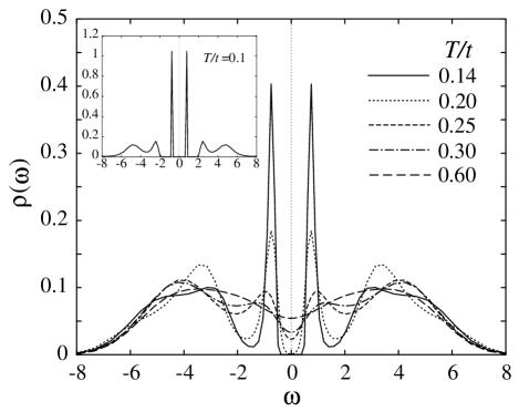
FIG. 1.: Spectra of single-particle excitations $\rho(\omega)$ at various temperatures. The inset shows the spectrum at the lowest temperature, $T=0.1$.

Let us discuss temperature dependence of $\rho(\omega)$. The most remarkable feature is that the quasiparticle gap is rapidly filled in with increasing temperature. At lower temperatures than the quasiparticle gap, the gap structure already disappears and it becomes a pseudo-gap. At the same time the sharp quasiparticle peaks lose their intensities. The intensities are transfered to higher frequencies and the dip structure is also smeared out. At high temperatures the spectrum shows only broad peaks which shift gradually to $\omega\simeq\pm 2$. The broad peaks correspond to the band edges of the free conduction electrons. In the 1D system, there are strong van Hove singularities at the band edges $\omega=\pm 2$. This behavior is reasonable since the conduction electrons are gradually decoupled from the $f$ spins as temperature is increased.

Now we turn to the local dynamic charge correlation function $N(\omega)$. A clear gap is developed in $N(\omega)$ at the lowest temperature, Fig. 2. The spectrum of $N(\omega)$ at $T=0.1$ has the edge at $\omega\simeq\Delta_{\rm c}=1.4$, which is twice of $\Delta_{\rm qp}=0.7$. There is a peak just above the gap. The peak structure corresponds to the charge excitations between the two sharp quasiparticle peaks of $\rho(\omega)$ shown in Fig. 1. The peak in $N(\omega)$ quickly changes into a shoulder as the temperature is increased.

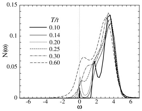
FIG. 2.: Spectra of charge excitations $N(\omega)$ at various temperatures.

It is interesting to note that the intensity of $N(\omega)$ is small above $\omega\gtrsim 4$, while the density of states $\rho(\omega)$ extends to much higher frequencies than $\omega=2$. This indicates that the structure of $N(\omega)$ cannot be understood by the simple picture of renormalized band corresponding to $\rho(\omega)$. In contrast to the low-energy excitations, the high-frequency excitations around $\omega\simeq 4$ may be understood in terms of the excitations of the nearly free conduction electron band. The large intensity of the peak is due to the van Hove singularities at the band edges of the 1D system.

At finite but low temperatures, there is a peak around $\omega\simeq 0$, which comes from the sharp peaks in $\rho(\omega)$. Quasiparticles and holes thermally populated at low temperatures contribute to the charge excitations within each peak. The integral intensity of the peak around $\omega\simeq 0$ grows up to $T\lesssim 0.2$ as the temperature is increased. As the temperature increases further, the charge excitation gap in $N(\omega)$ is rapidly filled in. At $T=0.3$ which is much smaller than the charge gap $\Delta_{\rm c}=1.4$, one can no longer find any gap structure, similarly to the temperature dependence of $\rho(\omega)$.

Next we show spin excitation spectra in Fig. 3. The spectrum of $S_{\rm c}(\omega)$ or $S_{\rm f}(\omega)$ at the lowest temperature shows a clear gap and the gap edge is lower than that of $N(\omega)$ as expected. The gap edge is consistent with the spin gap $\Delta_{\rm s}=0.4$ obtained by the zero-temperature DMRG.

At low temperatures $T=0.1,0.14$, and $0.2$, both $S_{\rm c}(\omega)$ and $S_{\rm f}(\omega)$ have two peaks. The peak at lower frequencies contain the $f$-spin excitations as the dominant component, while the main component of the peak at higher frequencies is the spin excitations of quasiparticles. In the high-frequency region of $S_{\rm c}(\omega)$, there is a shoulder structure at the lowest temperature, $T=0.1$. This may be related with the fact that the lowest spin excitation has the momentum $\pi$ and therefore a significant part of the spectral weight of quasiparticle excitations around $\omega\simeq 4$ is transfered to the low-energy excitations [18, 19].

As the temperature increases, the higher-frequency peak of $S_{\rm f}(\omega)$ and the lower-frequency peak of $S_{\rm c}(\omega)$ lose their intensities. Furthermore overall structures of $N(\omega)$ and $S_{\rm c}(\omega)$ are similar at high temperatures [20], and both have a peak structure around $\omega\simeq 4$. It shows that the main contribution to the peak is from the nearly free conduction electrons. These results indicate that the conduction electrons and the $f$-spins are decoupled as the temperature is increased.

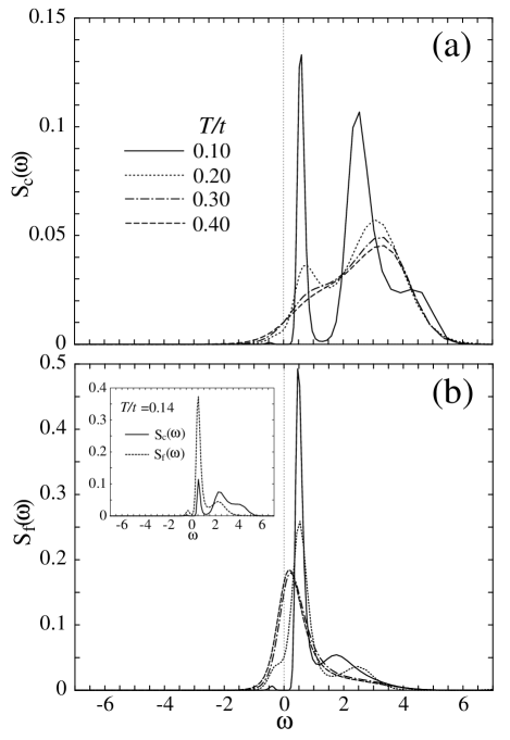
FIG. 3.: Spectra of (a) $S_{\rm c}(\omega)$ and (b) $S_{\rm f}(\omega)$ at various temperatures; $T=0.10,0.20,0.30$ and $0.40$. The inset of (b) shows the comparison of two spectra, $S_{\rm c}(\omega)$ and $S_{\rm f}(\omega)$ at $T=0.14$.

In conclusion, we have calculated dynamic correlation functions of the 1D KL model using the finite-$T$ DMRG method and the ME method. At low temperatures the density of states $\rho(\omega)$ has a quasiparticle gap and the sharp quasiparticle peaks at the gap edges. The gap is rapidly filled in and the sharp quasiparticle peaks are broadened as the temperature is increased. The temperature dependence of $\rho(\omega)$ shows clearly the many-body origin of the gap formation. The spectrum of $N(\omega)$ has a charge gap at low temperatures, and the charge gap also disappears as the temperature is increased. It is not possible to represent the many-body effects by a simple renormalized-band picture. One remarkable example is that the spectrum of $N(\omega)$ is different from the simple convolution of $\rho(\omega)$ particularly at high frequencies. Another example in the ground state is the difference between the spin gap and the charge gap, which have been discussed previously [9].

The temperature at which the quasiparticle gap and the charge gap disappear or the structure of $\rho(\omega)$ and $N(\omega)$ vary drastically is $T\simeq 0.3$. This temperature corresponds to the spin gap $\Delta_{\rm s}$. In the present system, the singlet binding between the conduction electrons and the $f$-spins produces the spin gap. As temperature is increased up to the order of $\Delta_{\rm s}$, the whole electronic states of the system are reconstructed. Therefore the smallest energy scale $\Delta_{\rm s}$ influences also the temperature dependence of charge excitations. This is another new feature of the Kondo insulators observed for the first time by the present method.

Concerning the application of the finite-$T$ DMRG to the dynamic quantities, we are benefited from discussions with Manfred Sigrist. We are also grateful to Hiroshi Kontani for helpful discussions. This work is financially supported by Grant-in-Aid from the Ministry of Education, Science, Sports and Culture of Japan.

* Present address: Institute of Applied Physics, University of Tsukuba, Tsukuba, Ibaraki 305, Japan

REFERENCES

- [1] S. R. White, Phys. Rev. Lett. 69, 2863 (1992); Phys. Rev. B48, 10345 (1993).
- [2] N. Shibata, J. Phys. Soc. Jpn. 66, 2221 (1997).
- [3] X. Wang and T. Xiang, Phys. Rev. B56, 5061 (1997).
- [4] R. N. Silver, D. S. Sivia, and J. E. Gubernatis, Phys. Rev. B41, 2380 (1990); J. E. Gubernatis, M. Jarrell, R. N. Silver, and D. S. Sivia, Phys. Rev. B44, 6011 (1991). For a recent review, see M. Jarrell and J. E. Gubernatis, Phys. Rep. 269, 133 (1996).
- [5] J. E. Hirsch and J. R. Schrieffer, Phys. Rev. B28, 5353 (1983).
- [6] H. -B. Schüttler and D. J. Scalapino, Phys. Rev. Lett. 55, 1204 (1985).
- [7] E. R. Gagliano and C. A. Balseiro, Phys. Rev. Lett. 59, 2999 (1987).
- [8] H. J. Vidberg and J. W. Serene, J. Low. Temp. Phys. 29, 179 (1977).
- [9] H. Tsunetsugu, M. Sigrist, and K. Ueda, Rev. Mod. Phys. 69, 809 (1997).
- [10] T. Nishino and K. Ueda, Phys. Rev. B47, 12451 (1993).
- [11] R. M. Fye and D. J. Scalapino, Phys. Rev. Lett. 65, 3177 (1990).
- [12] N. Shibata, B. Ammon, T. Troyer, M. Sigrist and K. Ueda, J. Phys. Soc. Jpn. 67, 1086 (1998).
- [13] C. C. Yu and S. R. White, Phys. Rev. Lett. 71, 3866 (1993).
- [14] N. Shibata, T. Nishino, K. Ueda and C. Ishii, Phys. Rev. B53, R8828 (1996).
- [15] N. Shibata and K. Ueda, to be published.
- [16] T. Mutou and D. S. Hirashima, J. Phys. Soc. Jpn. 64, 4799 (1995).
- [17] U. Fano, Phys. Rev. 124, 1866 (1961).
- [18] K. Tsutsui, Y. Ohta, R. Eder, S. Maekawa, E. Dagotto and J. Riera, Phys. Rev. Lett. 76, 279 (1996).
- [19] C. Gröber and R. Eder, Phys. Rev. B57, R12659 (1998).
- [20] The magnitude of the peak of is different from that of by the factor of which comes from spin .