Spin diffusion and relaxation in three-dimensional isotropic Heisenberg antiferromagnets

Abstract

A theory is proposed for kinetic effects in isotropic Heisenberg antiferromagnets at temperatures above the Neel point. A metod based on the analysis of a set of Feynman diagrams for the kinetic coefficients is developed for studying the critical dynamics. The scaling behavior of the generalized coefficient of spin diffusion and relaxation constant in the paramagnetic phase is studied in terms of the approximation of coupling modes. It is shown that the kinetic coefficients in an antiferromagnetic system are singular in the fluctuation region. The corresponding critical indices for diffusion and relaxation processes are calculated. The scaling dimensionality of the kinetic coefficients agrees with the predictions of dynamic scaling theory and a renormalization group analysis. The proposed theory can be used to study the momentum and frequency dependence of the kinetic parameters, and to determine the form of the scaling functions. The role of nonlocal correlations and spin-liquid effects in magnetic systems is briefly discussed.

PACS Nos:75.40.Gb, 75.50.Ee

I Introduction

In recent years there had been considerable activity, both experimental and theoretical, in the field of critical phenomena of antiferromagnets with Heisenberg and RKKY interactions [1] -[6]. This increase of interest [6]-[8] was stimulated by new experiments in high $T_{C}$ superconductors and heavy fermion compounds. In particular, the critical spin fluctuations are supposed to be responsible for Non-Fermi-Liquid low temperature behavior of the heat capacity and resistivity in $CeCu_{6-x}Au_{x}$ and $Ce_{1-x}La_{x}Ru_{2}Si_{2}$ [7],[8] in the vicinity of the quantum critical point. Besides, the Fermi-type Resonating Valence Bond excitations were introduced by [9],[10] in the framework of the Heisenberg model to describe unusual magnetic properties of high $T_{c}$ cuprates [10] and Ce - based heavy fermion compounds [11],[12]. In this case the critical spin fluctuations were shown to be important in the spin liquid formation mechanism. However, the scaling behavior of kinetic coefficients in the presence of spin - liquid fluctuations can be differ significantly from the predictions of the dynamic scaling theory [13].

In this paper we present a microscopic description of the scaling behavior of spin diffusion and relaxation coefficients in isotropic Heisenberg antiferromagnet in the critical region above the Neel temperature. The scaling dimension of kinetic coefficients was predicted by Halperin and Hohenberg [14]-[15]. They proposed the dynamic scaling hypothesis based on the assumption that the critical exponents of kinetic coefficients are the same on both sides of the phase transition point. The microscopic treatment of the spin diffusion in the paramagnetic phase of ferromagnet was proposed by S.V.Maleev [16] - [17]. Within the framework of this approach the approximations which are necessary for validity of the dynamic scaling hypothesis were established and momentum and frequency dependence of the spin diffusion coefficient was analyzed. We will follow Maleev’s approach to derive the scaling behavior of kinetic coefficients for Heisenberg antiferromagnet.

The qualitative picture of the critical phenomena expressed in terms of wave number $k$ and inverse coherence length $\xi^{-1}$ is well known [14]-[15]. There are two regions: ”hydrodynamic” regime deals with the longitudinal fluctuations $q\xi\ll 1$ of the order parameter - the staggered magnetization ${\bf N}={\bf N}_{1}-{\bf N}_{2}$ and ”critical” one considers the fluctuations with $q\xi\gg 1$ (the momentum ${\bf q}=|{\bf k-Q}|$ corresponds to small deviation of the momentum from the AF vector). However, there is an additional conserved quantity in AFM which is the total magnetization ${\bf M}={\bf M}_{1}+{\bf M}_{2}$. The fluctuations of this parameter do not lead to any singularities in spin correlators. Nevertheless, there is a region of longitudinal fluctuations of $M$ $k\xi\ll 1$ which is also can be called as ”hydrodynamic”. The goal of our work is to investigate the spin correlation functions behavior in the paramagnetic phase of AF and to establish the relations between the kinetic coefficients in two fluctuation regions of the phase diagram.

The dynamic of magnetization fluctuations is described by the van Hove microscopic diffusion equation in the long wave limit

$$\frac{\partial{\bf M}}{\partial t}=D_{0}\nabla^{2}{\bf M},$$ (1)

where $D_{0}$ is the spin diffusion coefficient. This equation is derived from the conservation low for the total magnetic moment, since the operator ${\bf M}$ commutes with the Hamiltonian. The fluctuation behavior of nonconserved order parameter is radically different. According to the general postulates of the thermodynamics of weakly nonequilibrium processes [18] the rate of change ${\bf N}$ is proportional to the conjugate thermodynamical force

$$\frac{\partial{\bf N}}{\partial t}=-\frac{\Gamma_{0}}{G_{0}}{\bf N},$$ (2)

here $G_{0}$ - is the static susceptibility, and the kinetic coefficient $\Gamma_{0}$ satisfies the condition $\Gamma_{0}>0$. The relaxation function determined by the equation (1) is nearly uniform, therefore the gradient terms for relaxation processes are omitted. In contrast to relaxation the first nonzero contribution to the spin diffusion equation is proportional to $q^{2}$. Although the average value of ${\bf M}$ is equal to zero on the both sides of the phase transition, the fluctuations of total magnetization around zero take place. However, unlike the FM case the diffusion mode is not the ”critical” mode for AF transition.

Thus, we are interested in the dynamical susceptibility of a cubic Heisenberg antiferromagnet in zero magnetic field above the Neel temperature,

$$H=-\sum_{<i,j>}V_{ij}{\bf S}_{i}{\bf S}_{j}$$ (3)

and the dipolar interaction [17] is neglected. As is known the susceptibility is related to the retarded Green’s function by the following equality:

$$\chi({\bf k},\omega)=(g\mu_{0})^{2}K^{R}_{SS}({\bf k},\omega),$$ (4)

where $g$ is Lande splitting factor, $\mu_{0}$ is Bohr magneton and

$$K^{R}_{SS}({\bf k},\omega)=i\int_{0}^{\infty}dte^{i\omega t}<[S^{z}_{\bf k}(t),S^{z}_{\bf-k}(0)]>,$$ (5)

$${\bf S}_{\bf k}=\frac{1}{\sqrt{N}}\sum_{i}e^{-i{\bf k}{\bf R}_{i}}{\bf S}_{i},$$

$${\bf M}=<{\bf S}_{0}>,\;\;\;\;\;\;{\bf N}=<{\bf S}_{\bf Q_{AFM}}>.$$

Using the equations (1, 2) one can obtain an expression for the retarded Green functions in the fluctuation region in the following form:

$$K^{R}_{SS}({\bf k\to 0},\omega)={\cal K}({\bf k},\omega)=G_{0}(k)\frac{iDk^{2}}{\omega+iDk^{2}}$$ (6)

$$K^{R}_{SS}({\bf q}=({\bf k}-{\bf Q})\to 0,\omega)={\cal L}({\bf q},\omega)=\frac{1}{-i\omega/\Gamma+G_{0}^{-1}(q)}$$ (7)

Here $G_{0}$ is the static spin correlation function. The equations (6, 7) correspond to diffusion and relaxation regimes respectively.

When $\tau=|T-T_{c}|/T_{c}\ll{\sf Gi}$ (${\sf Gi}$ is the Ginzburg number which characterizes the conditions when the Landau theory is valid) the fluctuations become important. The dynamic properties in this region can be described by Halperin - Hohenberg scaling hypothesis. According to this theory the equation for the dynamic susceptibility can be expressed in terms of the scaling function $F$:

$$K^{R}_{SS}({\bf k},\omega)=G_{0}({\bf k})F(k\xi,\frac{\omega}{T_{c}\tau^{\nu z}}),$$ (8)

Thus, the dynamic critical exponent $z$, which characterizes the critical fluctuations energy scale $\omega\sim k^{z}$, is connected with the static critical exponent $\nu\approx 2/3$ defined by the expression $\xi\sim\tau^{-\nu}$. We assume the static behavior of susceptibility in the form $G_{0}(q)\sim\xi^{2-\eta}$. We also neglect the Fisher index $\eta$ which determines the ”anomalous dimension” [18]. This approximation is valid in 3D case [18]. To derive the scaling properties of AF one have to introduce two types of the scaling functions: ${\cal F}_{1}$ and ${\cal F}_{2}$

$${\cal K}({\bf k},\omega)=G_{0}({\bf k}){\cal F}_{1}(k\xi,\frac{\omega}{T_{c}\tau^{\nu z}}),\;\;\;\;\;\;{\cal L}({\bf q},\omega)=G_{0}({\bf q}){\cal F}_{2}(q\xi,\frac{\omega}{T_{c}\tau^{\nu z}}),$$ (9)

In principal, expressions (8, 9) determine the kinetic coefficients $D_{0}$ and $\Gamma_{0}$ in terms of coherence length. Moreover, the renormalization group analyses [14],[19] has shown that the kinetic coefficients are singular in the fluctuation region of AF.

The theory under consideration is a variant of the mode-mode coupling theory proposed by Kawasaki [20] (see also [21]-[23]). We extend to AF systems the dynamic scaling method offered by Maleev for ferromagnets. As was mentioned above, the aim of our paper is to derive the scaling behavior and momentum and frequency dependence of ${\cal F}$ functions in the fluctuation region of AF. Assumptions which are crucial for the microscopic substantiations of dynamic scaling hypothesis will be also formulated.

II Generalized kinetic coefficients

We consider the dynamic susceptibility of cubic Heisenberg antiferromagnet in the fluctuation region above the Neel temperature. The equations (6, 7) can be rewritten in more general form:

$$K^{R}_{SS}({\bf k},\omega)=\frac{i\gamma({\bf k},\omega)}{\omega+iG_{0}^{-1}({\bf k})\gamma({\bf k},\omega)}$$ (10)

There is a simple expression for the spin - diffusion coefficient in the hydrodynamical regime

$$D_{0}=\lim_{{\bf k}\to 0}\lim_{\omega\to 0}k^{-2}\gamma({\bf k},\omega)G_{0}^{-1}({\bf k}),$$ (11)

The generalized kinetic coefficient in the relaxation region is $\gamma({\bf k},\omega)=\Gamma({\bf k},\omega)$. The different limits $k\to 0,\omega\to 0$ in the expressions (6, 7) significantly depend on the relations between $k$ and $\omega$. These limits are completely analogous to those considered in the Fermi Liquid theory [24]. In the treatment below we consider the the quasistatic limit of ${\bf k}\to 0$, $|\omega|/{\bf k}^{2}\to 0$.

As it was shown by Maleev, it is possible to determine the kinetic coefficients in terms of the Kubo functions for the operators $S$ and $\dot{S}$, where $\dot{S}=dS/dt$,

$$\gamma({\bf k},\omega)=\frac{\Phi_{\dot{S}\dot{S}}({\bf k},\omega)}{1+G_{0}^{-1}(k)\Phi_{\dot{S}S}({\bf k},\omega)},$$ (12)

and

$$\Phi_{AB}({\bf k},\omega)=\frac{1}{i\omega}[K^{R}_{AB}({\bf k},\omega)-K^{R}_{AB}({\bf k},0)],$$

$$K^{R}_{AB}({\bf k},\omega)=i\int_{0}^{\infty}dte^{i\omega t}<[A_{\bf k}(t),B_{\bf-k}(0)]>.$$

The formal expression (12) is exact, and it takes into account the nonlinear character of the relaxation forces. In the case of purely exchange interaction, $\dot{S}\sim k$ and $\gamma=\Phi_{\dot{S}\dot{S}}({\bf k},\omega)$. The Kubo function in the denominator vanishes at ${\bf k=0}$, and we arrive at the expression $\gamma=\Phi_{\dot{S}\dot{S}}$. However, in studying the dispersion of the kinetic coefficients, i.e. its dependence on $k$, $\omega$, we cannot, generally speaking, neglect this function in the denominator.

Using the properties of spin operators, it is not difficult to obtain the relations between different retarded spin Green’s functions $K^{R}_{SS}({\bf k},\omega)$, $K^{R}_{\dot{S}S}({\bf k},\omega)$ and $K^{R}_{\dot{S}\dot{S}}({\bf k},\omega)$ in the paramagnetic phase. These relations are result of dispersion relations [26]:

$$K^{R}_{\dot{S}S}({\bf k},\omega)=-i\omega K^{R}_{SS}({\bf k},\omega),\;\;\;\;K^{R}_{S\dot{S}}({\bf k},\omega)=-K^{R}_{\dot{S}S}({\bf k},\omega)=i\omega K^{R}_{SS}({\bf k},\omega),\;\;\;\;$$

$$\omega^{2}K^{R}_{SS}({\bf k},\omega)=[K^{R}_{\dot{S}\dot{S}}({\bf k},\omega)-K^{R}_{\dot{S}\dot{S}}({\bf k},0)]$$ (13)

In particular, it is seen from equation (13) that the function $K^{R}_{\dot{S}\dot{S}}({\bf k},\omega)$ possesses the same symmetry properties as spin - spin correlation function.

The spin current operators taken in the form

$$K_{\dot{S}\dot{S}}({\bf k},\omega_{n})=\frac{(a^{2}T_{c}\alpha)^{2}}{6N}\int_{0}^{1/T}d\tau e^{i\omega_{n}\tau}\sum_{\bf p_{1},p_{2}}(\nabla V({\bf p_{1}}){\bf k})(\nabla V({\bf p_{2}}){\bf k})<T_{\tau}(S^{\mu}_{\bf p_{1}+k}S^{\rho}_{-\bf p_{1}})_{\tau}(S^{\mu}_{\bf-p_{2}-k}S^{\rho}_{\bf p_{2}})_{0}>$$ (14)

can be connected with the Kubo functions for Matsubara frequencies $\omega_{n}$ with the use of equation of motion:

$$\dot{S}^{\alpha}_{\bf k}=-\frac{1}{\sqrt{N}}\sum_{\bf p}[V({\bf p}+{\bf k})-V({\bf p})]\epsilon_{\alpha\beta\gamma}S^{\beta}_{{\bf p}+{\bf k}}S^{\gamma}_{-{\bf p}}$$ (15)

The spin - current correlators can be calculated diagrammatically and then the explicit equations (10-12) for the kinetic coefficients can be obtained. When deriving eq. (14), we have confined ourselves to the lowest terms of the expansion in powers of $ka$ and have put $\nabla V({\bf p})\approx{\bf p}T_{c}a^{2}\alpha$, where $\alpha\sim 1$. Since, we are interested in the correction terms of order $(k\xi)^{2}$ and $(k\xi)^{3}$; we consistently neglect the $(ka)^{2}$ and $(ka)^{3}$ corrections, because $\xi\gg a$. Thus the problem of derivation of the kinetic coefficients is reduced to the analysis of four - spin correlators with current vertices. The later problem can be solved by analytical continuation of the temperature Feynman’s diagram to the upper half-plane of complex variable $\omega$ The Feynman diagrams corresponding to the spin-current correlation function are shown on figure 1.

The ”bare” poles of the Green’s functions (6, 7) lie on imaginary axis. Introducing fictitious quasi - particles ”diffusons” and ”relaxons” we obtain the self-consistent equations for kinetic coefficients and determine their scaling dimensions.

The static susceptibility in the fluctuation region obeys the Ornstein - Zernike law

$$G_{0}({\bf q})=K^{R}_{SS}({\bf q},0)=\frac{A}{T_{c}\tau^{2\nu}}\frac{1}{(q\xi)^{2}+1},$$ (16)

(here A is a constant ($A\sim 1$), $\tau\ll 1$). There is no singularities of static susceptibility in the diffusion region $k\xi\ll 1$, where $G_{0}\approx A/(2T_{c})$.

In Sec. III the relations between kinetic coefficients are established and scaling dimensions of kinetic coefficient are analyzed. Sec. IV is devoted to a momentum and frequency dependence of spin diffusion and spin relaxation constants.

III Relations between kinetic coefficients

We begin with analyzing the set of diagrams which cannot be separated into two parts by cutting one line of interaction, and include these diagrams into the irreducible self-energy part of the spin - current correlation function. Using the definition of $\gamma$ and properties of the functions $K$ we obtain an expression for generalized kinetic coefficient in terms of irreducible self - energy parts:

$$\gamma({\bf k},\omega)=\frac{1}{i\omega}[\Sigma^{R}_{\dot{S}\dot{S}}({\bf k},\omega)-\Sigma^{R}_{\dot{S}\dot{S}}({\bf k},0)+\frac{{\cal R}^{R}_{\dot{S}S}({\bf k},\omega)\gamma({\bf k},\omega){\cal R}^{R}_{S\dot{S}}({\bf k},\omega)}{-i\omega+G_{0}^{-1}(k)\gamma({\bf k},\omega)}][1+G_{0}^{-1}\frac{{\cal R}^{R}_{\dot{S}S}({\bf k},\omega)\gamma({\bf k},\omega)}{i\omega(-i\omega+G_{0}^{-1}(k)\gamma({\bf k},\omega))}]^{-1}$$ (17)

The equation (17) can be derived both from analysis of diagrammatic series for the spin - current correlators [16], and directly from Larkin equation [12],[26]. Below we use the following notations for retarded spin Green’s functions: $K^{R}_{\dot{S}S}({\bf k},\omega)={\cal R}^{R}({\bf k},\omega)K^{R}_{SS}({\bf k},\omega)$, and $\Sigma^{R}_{AB}$ - are the irreducible self - energies. To obtain the graphical representation for the irreducible part $\Sigma^{R}_{\dot{S}\dot{S}}$ one have to replace the ”dressed” vertex in fig.1 by the irreducible one. The estimation of ${\cal R}$ in the framework of mean - field theory [16], [27] results in:

$${\cal R}\sim(k\xi)(ka)\ll(k\xi)^{2}$$ (18)

Moreover, due to analytical properties of spin correlators, ${\cal R}^{R}\sim\omega$. We assume that the expression for ${\cal R}$ contains the small parameter $a/\xi$ in a limit of small $\omega$ not only in critical region and neglect this contribution below. Therefore, the generalized kinetic coefficient $\gamma$ can be rewritten in terms of irreducible self - energies only:

$$\gamma({\bf k},\omega)=\frac{1}{i\omega}(\Sigma^{R}_{\dot{S}\dot{S}}({\bf k},\omega)-\Sigma^{R}_{\dot{S}\dot{S}}({\bf k},0))$$ (19)

The general set of diagrams for the irreducible self - energy part $\Sigma_{\dot{S}\dot{S}}$ in imaginary time can be classified by the number of intermediate states. First, we confine ourselves to the diagrams with two - particles intermediate states (fig.2)

$$\Sigma_{\dot{S}\dot{S}}^{(2)}({\bf k},i\omega)=\frac{(T_{c}a^{2}\alpha)^{2}}{\sqrt{N}}T\sum_{\epsilon}\sum_{\bf p}({\bf k}{\bf\Lambda^{(2)}}({\bf p,k},i\omega,i\epsilon,i(\omega-\epsilon)))({\bf k}{\bf\Lambda^{(2)}}^{\dagger}({\bf p,k},i\epsilon,i(\omega-\epsilon),i\omega))\times$$

$$\times K_{SS}({\bf p},i\epsilon)K_{SS}({\bf k-p},i\omega-i\epsilon)$$ (20)

Replacing the sum over momentum ${\bf p}$ by the integration one should use the ”cutoff” $p\sim\xi^{-1}$ as an upper limit of integration. This means that the integrations are restricted by the region close to the appropriate singularities (small ${\bf p}$ and small ${\bf q}$ for ${\bf p}\sim{\bf q}+{\bf Q}$ in the vicinity of AF vector ${\bf Q}$). From the point of view of the energy dependence, the vertices ${\bf\Lambda}^{(2)}$ being the three - point functions are the analytical functions of all three frequencies $\omega$ and, in each of the frequencies they have a cut along the real axis; they have no singularities in the physical region of variables $\omega$ [28]. Due to these properties it is possible to separate the vertex into a static part and dynamic contribution, disappearing in the limit $\omega\to 0$ [28]. We concentrate below on the static vertex.

As it can be seen from the fig.2(a), the static vertices correspond to the longitudinal processes of ”diffuson” - ”diffuson” or ”relaxon”- relaxon” pair creation and annihilation, since in this case only the modes of the same origin couple together. On the other hand, the static Green function $G({\bf k})$ is not sensitive to the direction of the momentum. In the other words, the corresponding lines in the diagrams are not directed. For this reason, the processes of diffuson and relaxon scattering contain the same vertices as the processes of pair creation and annihilation. However, for such a scattering processes in the limit $k\to 0$ the Ward identity holds [18],[24] (fig.3):

$${\bf\Lambda}^{(2)}({\bf p,k},0)\sim\partial G_{0}^{-1}/\partial{\bf p}$$ (21)

As was mentioned, the region of integration in the second term is concentrated near the points ${\bf p}\approx{\bf Q}$. The contribution from the staggered magnetization fluctuations into the spin diffusion can be calculated by means of the substitution ${\bf p}={\bf q}+{\bf Q}$ and, by use of the property $\partial G_{0}^{-1}/\partial{\bf p}=\partial G_{0}^{-1}/\partial{\bf q}$.

Let us consider the diagram fig.2(b). The external momentum of this diagram can be taken equal to ${\bf Q}_{AF}$. Therefore, we have two different coupling modes, ”diffuson” and ”relaxon”. Thus, this diagram corresponds to the process of ”diffuson” - ”relaxon” pair creation. For this reason we can not use the Ward identity to analyze this contribution. However, the ”bare” vertex (fig.3) has the scaling dimension

$${\bf\Lambda}^{(2)}_{0}({\bf p,Q},0)\sim\partial V/\partial{\bf p}\sim{\bf p}$$

Besides, in the magnetic Brillouin Zone the points 0 and $Q$ are equivalent. Taking into account the direction independence of interacting modes in fluctuating region one can assume that the processes of multiple scattering on the static fields do not influence the scaling dimension of the static vertex.

Using the properties of vertices it is not difficult to perform the summation over $\epsilon$ and the analytical continuation in $\omega$ [24]. As a result we obtain the following expressions for kinetic coefficients

$$D_{0}^{(2)}=\tilde{A}T_{c}\int_{-\infty}^{\infty}\frac{d\varepsilon}{2\pi}coth(\frac{\varepsilon}{2T})\sum_{\bf p}(\nabla G_{0}^{-1}({\bf p}))^{2}[{\it Im}{\cal K}({\bf p},\varepsilon)\frac{\partial}{\partial\varepsilon}{\it Im}{\cal K}({\bf p-k},\varepsilon)+{\it Im}{\cal L}({\bf p},\varepsilon)\frac{\partial}{\partial\varepsilon}{\it Im}{\cal L}({\bf p-k},\varepsilon)]$$ (22)

$$\Gamma_{0}^{(2)}=\tilde{B}\int_{-\infty}^{\infty}\frac{d\varepsilon}{2\pi}coth(\frac{\varepsilon}{2T})\sum_{\bf p}(\nabla G_{0}^{-1}({\bf p}){\bf Q})^{2}\times[{\it Im}{\cal K}({\bf p},\varepsilon)\frac{\partial}{\partial\varepsilon}{\it Im}{\cal L}({\bf p-q},\varepsilon)+{\it Im}{\cal L}({\bf p},\varepsilon)\frac{\partial}{\partial\varepsilon}{\it Im}{\cal K}({\bf p-q},\varepsilon)]$$ (23)

There index ⁽²⁾ stands for the processes with only two - particle intermediate states taken into account. The equations generalize the corresponding equation (23) are obtained by Maleev [16] for ferromagnets. In that case it is possible to retain only the first term in expression (22), since one deals with a single mode regime. Equations (22,23) can be rewritten in a different form. Taking ${\bf k}=0$ and ${\bf q}=0$ and integrating by parts over $\epsilon$ one can obtain the following result:

$$D_{0}^{(2)}=\frac{\tilde{A}}{4}\int_{-\infty}^{\infty}\frac{d\varepsilon}{2\pi}sh^{-2}(\frac{\varepsilon}{2T})\sum_{\bf p}(\nabla G_{0}^{-1}({\bf p}))^{2}[({\it Im}{\cal K}({\bf p},\varepsilon))^{2}+({\it Im}{\cal L}({\bf p},\varepsilon))^{2}]$$ (24)

$$\Gamma_{0}^{(2)}=\frac{\tilde{B}}{2T_{c}}\int_{-\infty}^{\infty}\frac{d\varepsilon}{2\pi}sh^{-2}(\frac{\varepsilon}{2T})\sum_{\bf p}(\nabla G_{0}^{-1}({\bf p}){\bf Q})^{2}{\it Im}{\cal K}({\bf p},\varepsilon){\it Im}{\cal L}({\bf p},\varepsilon)$$ (25)

These expressions are in fact a generalization of equations derived by Maleev [16] for the case of two coupling modes.

As it was mentioned above, the main contribution to the integrals (22,23) appears from the vicinity of scaling functions singularities (9). Besides, the characteristic energies of critical fluctuations satisfy the condition $\omega^{*}\ll T_{c}$ due to the ”critical slowing down”. Thus, we can replace the hyperbolic functions (22 -24) by their arguments. Calculating integrals over the frequencies and extracting the scaling dimension of kinetic coefficients we obtain the relation between spin diffusion coefficient and the relaxation constant.

$$D_{0}=b_{1}T_{c}^{2}a^{4}(\frac{\xi}{a})^{-3}\frac{1}{D_{0}}+b_{2}T_{c}a^{2}(\frac{\xi}{a})\frac{1}{\Gamma_{0}}$$ (26)

It is interesting to note that the expressions (26) can be derived by direct substitution of retarded Green functions (6,7) to the expressions (22,24). After integration over the frequencies we obtain the equations on kinetic coefficients which contain only integration over momentum of the different powers of the static correlator $G_{0}$. As a result the first term is determined by the two - diffuson intermediate state and the second term corresponds to two - relaxon intermediate state.

The integrals (23 - 25) can be calculated in the same way. The equation which determines the relaxation constant in terms of spin diffusion coefficient can be written in following form:

$$\Gamma_{0}=c_{1}(\frac{\xi}{a})\frac{1}{\Gamma_{0}}+c_{2}(\frac{\xi}{a})\frac{D_{0}/(T_{c}a^{2})}{\Gamma_{0}^{2}}$$ (27)

The coefficients $b_{1,2},c_{1,2}\sim 1$ in eqs. (26,27) depend on the shape of a scaling function and, strictly speaking, can not be calculated in the framework of method used. Solution of self - consistent system of algebraic equations leads to following scaling dimension of kinetic coefficient

$$D_{0}/(T_{c}a^{2})\sim\Gamma_{0}\sim(\xi/a)^{1/2}$$ (28)

Behavior of kinetic coefficient agrees with predictions of dynamic scaling theory [14]-[15] and with renormalization group analysis [15][19]. Therefore, the kinetic coefficients of AF are singular in fluctuating region, and spin diffusion is determined by the intermediate relaxation processes. A correction in (24) corresponding to the influence of self - diffusion is proportional to $\delta D_{0}/D_{0}\sim(\xi/a)^{-4}\sim\tau^{8/3}\ll 1$. Hence, these processes can be omitted in the critical region. Calculation of dynamic critical exponent z (see eq.8) results in $z=3/2$.

The simple physical assumptions explaining the spin diffusion and relaxation in the fluctuation region are based on the following argument: in the vicinity of the phase transition point $T\to T_{c}$ the regions of short range order are formed. The characteristic length scale of the ordered regions is $\xi$. The excitations in these regions are the AF magnons with sound like dispersion law. Estimations of the spin diffusion coefficient results in $D_{0}\sim\xi^{2}/t_{diff}$, where $t_{diff}\sim\xi/c$ is a characteristic diffusion time and $c\sim\xi^{-1/2}$ is a ”sound” velocity [14], therefore $D_{0}\sim\xi^{1/2}$. Due to the dynamic scaling hypothesis which postulates the invariance of the dynamic scaling exponent $z$, the characteristic scaling behavior of relaxation constant is $\Gamma_{0}\sim\xi^{1/2}$.

Although the kinetic coefficients are singular, the characteristic relaxation times of staggered magnetization and spin diffusion become infinite. This result guarantees the existence of macroscopic ordered regions, corresponding to the partial equilibrium of the system [30].

It should be emphasized that we did not use any assumptions about the elementary excitations spectrum in ordered phase when deriving the expressions (26). Our study is based only on a concept of total magnetization conservation and order parameter non-conservation.

IV Corrections to the kinetic coefficients

Here we study the kinetic coefficient as a functions of finite but small ${\bf k}$ and $\omega$. For this sake we use the relations between spin correlation functions (12) and Kubo functions (17). It can be seen that the corrections due to momentum and frequency dependence of kinetic coefficient are determined both by the nonlinear character of the relaxation forces and the momentum and frequency dependence of irreducible self - energy parts. According to the estimation (18) one can derive the frequency and momentum dependence of spin diffusion and relaxation constants only in terms of linear response theory. Therefore, we can neglect the nonlinear character of relaxation forces.

First, we consider the static renormalizations of kinetic coefficients. It is not difficult to obtain the usual expansions for spin diffusion and relaxation constants in series of $(k\xi)^{2n}$, $(q\xi)^{2n}$:

$$D^{(2)}({\bf k},0)=D_{0}(0,0)[1+\alpha^{{}^{\prime}}(k\xi)^{2}+...]$$

$$\Gamma^{(2)}({\bf q},0)=\Gamma_{0}(0,0)[1+\beta^{{}^{\prime}}(q\xi)^{2}+...]$$

As is known [29], these expansion can be done due to the singularities of static spin correlation functions in points ${\bf k}_{i}=-n^{2}\xi^{-2}$, where $n$ are integer. The coefficients $\alpha^{{}^{\prime}}$, $\beta^{{}^{\prime}}$ are determined by the shape of static correlation function.

We analyze the energy dependence of kinetic coefficients. Using equation (19) we obtain the following expressions for the real and imaginary parts of the generalized coefficient $\gamma({\bf k},\omega)$:

$${\it Re}\gamma({\bf k},\omega)=\frac{{\it Im}\Sigma^{R}_{\dot{S}\dot{S}}({\bf k},\omega)}{\omega},\;\;\;{\it Im}\gamma({\bf k},\omega)=-\frac{{\it Re}\Sigma^{R}_{\dot{S}\dot{S}}({\bf k},\omega)-{\it Re}\Sigma^{R}_{\dot{S}\dot{S}}({\bf k},0)}{\omega}$$ (29)

Since ${\it Im}\gamma$ is the odd function of $\omega$ and ${\it Re}\gamma$ is the even function of $\omega$ the first nonzero term in the energy expansion of kinetic coefficients is proportional to $\omega^{2}$.

Let us introduce the effective generalized kinetic coefficient $\gamma^{*}$ by the definition:

$$\gamma^{*}=\frac{\displaystyle\frac{\partial}{\partial\omega}{\it Im}\Sigma^{R}_{\dot{S}\dot{S}}({\bf k},\omega)|_{\omega=0}}{1+\displaystyle G_{0}^{-1}({\bf k})\frac{\partial}{\partial(\omega)^{2}}{\it Re}\Sigma^{R}_{\dot{S}\dot{S}}({\bf k},\omega)|_{\omega=0}}$$ (30)

The expression for the coefficient $\gamma^{*}$ is completely analogous to the definition of effective mass in the theory of quantum liquids. The renormalization constant $Z$ is similar to the Fermi - liquid $Z$ factor.

$$Z=\frac{1}{1+\displaystyle G_{0}^{-1}({\bf k})\frac{\partial}{\partial(\omega)^{2}}{\it Re}\Sigma^{R}_{\dot{S}\dot{S}}({\bf k},\omega)|_{\omega=0}}$$

Calculating $Z$ in fluctuation region results in the following expressions for renormalization constant:

$$Z({\bf k}\to 0)=\frac{1}{1+\epsilon^{{}^{\prime}}(k\xi)^{2}},\;\;\;\;Z({\bf q}\to 0)=\frac{1}{1+\delta^{{}^{\prime}}+\delta^{{}^{\prime\prime}}(q\xi)^{2}}$$ (31)

where the coefficients $\epsilon^{{}^{\prime}},\delta\ll 1$ also can be expressed in terms of the integrals of different powers of static correlator $G_{0}$. Using the definition (30) for small, but nonzero frequencies one can obtain the expansions of real spin diffusion coefficient $D^{*}$ and relaxation constant $\Gamma^{*}$ :

$$D^{(2)*}({\bf k},\omega)=D_{0}(0,0)[1+\alpha^{{}^{\prime}}(k\xi)^{2}+\alpha^{{}^{\prime\prime}}_{k\xi}(\omega/\omega^{*})^{2}+...]$$

$$\Gamma^{(2)*}({\bf q},\omega)=\Gamma_{0}(0,0)[\beta+\beta^{{}^{\prime}}(q\xi)^{2}+\beta^{{}^{\prime\prime}}_{k\xi}(\omega/\omega^{*})^{2}+...]$$ (32)

It should be noted that we do not intend to describe the kinetic coefficients properties in the region $\omega\sim\omega^{*}$, $k,q\sim\xi^{-1}$. The diffusion and relaxation picture in this region becomes very complicated and scarcely amenable to detailed analysis at the present time. For this reason we shall neglect the irregular corrections to kinetic coefficients resulting from the generation of poles chain and drift of the poles toward the new cut [16],[17]. In the region of ${\bf k}$, $\omega$ under consideration, all these singularities are small corrections, and therefore, the phenomena associated with them are no special interest.

Now we turn to discussion of the role of many - particles $(m>2)$ intermediate states. As it was mentioned above, we are interested only in regular contributions of such diagrams to the kinetic coefficients:

$$\frac{{\it Im}\Sigma^{R(m)}_{\dot{S}\dot{S}}}{\omega}\sim(ka)^{2}\sum_{\bf p_{1}}...\sum_{\bf p_{m}}{\bf\Lambda^{(m)}}({\bf k},{\bf p}_{1},...,{\bf p}_{m}){\bf\Lambda^{(m)}}^{\dagger}({\bf k},{\bf p}_{1},...,{\bf p}_{m})\delta({\bf p_{1}+...p_{m}-k})\times$$

$$\times\frac{1}{\pi^{m-1}}\int_{-\infty}^{\infty}...\int_{-\infty}^{\infty}\frac{d\varepsilon_{1}...d\varepsilon_{m}{\it Im}K^{R}_{SS}({\bf p}_{1},\varepsilon_{1})...{\it Im}K^{R}_{SS}({\bf p}_{m},\varepsilon_{m})}{\varepsilon_{1}...\varepsilon_{m}}\delta(\varepsilon_{1}+...+\varepsilon_{m}-\omega),$$ (33)

Here the functions $K$ correspond both to ”diffusons” and ”relaxons”. The integration over frequency is still restricted by the regions close to singularities of scaling function. In the case of $m=2$ the expression (33) simply transforms into (24,25).

The vertices ${\bf\Lambda^{(m)}}$ are symmetric functions of the momenta of intermediate particles. For ${\bf k}=0$ the generalized Ward identities similar to thous of ref. [16] hold for ${\bf\Lambda^{(m)}}$; therefore, ${\bf\Lambda^{(m)}}$ can be expressed as a sum of derivatives of the ordinary n - particle vertices of static scaling theory. A ”dimensional” estimate exists for the latter [29]: $\Gamma_{m}\sim p^{3-m/2}$ in the limit ${\bf k}\to 0$. As a result, the diagrams with m-particle intermediate states in the channel of ”diffusons” and ”relaxons” creation do not change the scaling dimension of irreducible self - energies. As to the vertices behavior around the AF vector $Q$, there is a direct mapping of the properties of the diagrams with two - particle intermediate states onto those with many - particle intermediate states. Therefore, we can confine ourselves only by the diagrams with two - particle intermediate states. Another diagrams only renormalize the numerical constants, and the latter can not be determined in a framework of our method. The energy dependence of vertices also can not change the scaling behavior of kinetic coefficients [16].

Conclusion

We investigated the scaling behavior of generalized kinetic coefficients in 3D isotropic Heisenberg antiferromagnets. In a framework of analysis based on the modified mode - mode coupling theory the critical exponents are derived. Necessary approximations in microscopic approach to satisfy the dynamic scaling hypothesis are formulated. In particular, it is shown that the main sequence of Feynman diagrams contain the processes with two - particles intermediate states. Besides, the vertices of static scaling theory are proved to give the main contribution to quasiparticles scattering processes.

The momentum and frequency dependence of spin diffusion and relaxation coefficients is found in the ”pole” approximation. A definition of the generalized effective coefficient is introduced in a full analogy with that used in the theory of quantum liquids for a definition of effective mass. Taking into account the renormalization processes responsible for multiple scattering of ”diffusons” and ”relaxons” we derived the asymptotics of scaling function in the region of small frequencies and momenta, $\omega\ll\omega^{*}$, $k,q\ll\xi^{-1}$.

Our investigation of the critical dynamic is based on the static and dynamic scaling hypotheses. We took into account only two coupling modes. One of them is considered to be responsible for fluctuations of the total magnetization and another deals with the fluctuations of order parameter - staggered magnetization. Existence of two modes is determined by the conservation’s laws of the Heisenberg model. For this reason, our results depend only weakly on the specific properties of AF and we expect that all they are valid for any system with nonconserved order parameter when the additional conserved quantity exists.

The scaling behavior of more complicated systems, e.g. Ce - based heavy fermion compounds with almost integer valence, can be significantly different from critical dynamic of Heisenberg magnets. In these systems an additional coupling modes interacting with paramagnons can appear due to, e.g., the spin liquid correlations, proposed in Ref.[12]. An additional modes in Kondo lattices can be also connected with itinerant - magnetic excitations. Kinetic coefficients of such systems can be measured by the methods of of inelastic neutron scattering to verify a spin liquid correlations existence.

The methods developed in this paper can be useful for the systems close to the quantum critical point [6],[31] – [32] when the temperatures of AF ordering are close to zero, or, even negative. Our method also should be valid for anisotropy magnets, antiferrimagnets and systems with dipolar interactions.

We think that the diagrammatic approach for investigation of kinetic coefficient in the vicinity of Neel point has some advantages in comparison with other methods [14]-[15], [20]. This approach can be applied to the unrenormalizible Hamiltonians and to systems with nonlocal coupling modes [13].

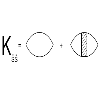
FIG. 1.: Diagrammatic equation for spin - current correlator.

FIG. 2.: Feynman diagrams for kinetic coefficients. Only two - particles intermediate states are taken into account. The diffusion mode is represented by the wavy lines. Dashed lines stand for the relaxation mode. Dots represent the vertex parts from static scaling theory.

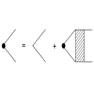
FIG. 3.: Equations for two - particle dynamic vertex.

REFERENCES

- [1] S.Chakravarty, B.I.Halperin, and D.R.Nelson, Phys.Rev B39, 2344 (1989)
- [2] D.P.Arovas and A.Auerbach, Phys.Rev. B38, 316 (1988).
- [3] A. Chubukov, Phys. Rev. B44, 12 318 (1991).
- [4] H.Monien, D.Pines and C.P.Slichter, Phys.Rev. B44, 11 120 (1990).
- [5] K.Ueda,T.Moriya and Y.Takahashi. Electron Properties and Mechanisms of High-Tc superconductors. North - Holland, Amsterdam, 1992.
- [6] A.Millis, Phys.Rev. B 48, 7183 (1993).
- [7] S.Kambe at al., J.Phys.Soc of Japan 65, 3294 (1996).
- [8] A.Rosch, A.Schrder, O.Stockert and H.v.Lhneysen. Phys.Rev. Lett.79, 159 (1997), O.Stockert, H.v. Lhneysen, A.Rosch, N.Pyka and M.Loewenhaupt. cond-mat/9802086.
- [9] P.W. Anderson, Mater. Res. Bull., 8, 153 (1973).
- [10] G. Baskaran, Z. Zou, and P. W. Anderson, Solid State Comm. 63, 973. (1987).
- [11] Yu. Kagan, K.A. Kikoin, and N.V. Prokof’ev, Physica B 182, 201 (1992)
- [12] K.A.Kikoin, M.N.Kiselev, A.S.Mishchenko, Sov. JETP Letters 60, 600 (1994). Physica B 206&207, 129 (1995)
- [13] K.A.Kikoin, M.N.Kiselev, A.S.Mishchenko, Sov.Phys.JETP. 111, 729 (1997).
- [14] B.I. Halperin, P.C. Hohenberg, Phys.Rev. 177, 952 (1969), Phys.Rev. 188, 898 (1969),Rev. Mod. Phys. 49, 435 (1977).
- [15] B.I. Halperin, P.C. Hohenberg, and E.D.Siggia, Phys.Rev. B13, 1299 (1976).
- [16] S.V.Maleev, Sov.Phys.JETP 38, 613 (1974).
- [17] S.V.Maleev, Sov.Phys.JETP 39, 889 (1974), Sov.Physics Rev. A8, 323 (1987).
- [18] A.Z.Patashinskii, V.L.Pokrovskii. Fluctuation Theory Of Phase Transition. Pergamon Press, 1979
- [19] R.Freedman and G.F.Mazenko, Phys.Rev.Lett 34, 1571, (1975).
- [20] K.Kawasaki, In Phase Transitions and Critical Phenomena, ed. C.Domb and M.S.Green, Academic New York, Vol 5a, 1976.
- [21] S.W.Lovesey, E.Engahl, A.Cuccoli and V.Tognetti. J.Phys.Cond.Matt. 6, 7099 (1994), J.Phys.Cond.Matt. 6, 7553 (1994)
- [22] E.Frey,F.Schvabl and S.Thoma Phys.Rev. B 40, 7199 (1989)
- [23] S.W.Lovesey, E.Engahl, A.Cuccoli and V.Tognetti. J.Phys.Cond.Matt. 7, 2615 (1995)
- [24] A.A.Abrikosov, L.P. Gor’kov, I.E. Dzyaloshinski. Methods of quantum field theory in statistical physics. Prentice-hall. New Jersey 1963.
- [25] L.Kadanoff and P.Martin, Ann. Phys. 24,419 (1963).
- [26] Yu. A. Izyumov, Yu.N. Skryabin. Statistical Mechanics of Magnetically Ordered Systems. Plenum, New York, 1988.
- [27] V.G.Vaks, A.I.Larkin, S.A.Pikin. Sov.Phys.JETP 24, 240 (1967), Sov.Phys.JETP 26, 188 (1968).
- [28] G.M. Eliashberg Sov.Phys.JETP 14, 886 (1962), Sov.Phys.JETP 15, 1151 (1962), S.V.Maleev, Sov.Theor.Mat.Phys. 4, 86 (1970).
- [29] A.A.Migdal, Sov.Phys.JETP 28, 1036 (1969), A.M.Polyakov, Sov.Phys.JETP 30, 151 (1970).
- [30] E.M.Lifshits, L.P.Pitaevskii, Physical Kinetics. Pergamon Press, 1981.
- [31] J.Hertz, Phys.Rev. B 14, 1165 (1975),
- [32] T.Moriya. Spin fluctuations in Itinerant Electron Magnetism (Springer, Berlin, 1985)