On the Relationship Between the Pseudo- and Superconducting Gaps: Effects of Residual Pairing Correlations Below $\textstyle T_{c}$

Abstract

The existence of a normal state spectral gap in underdoped cuprates raises important questions about the associated superconducting phase. For example, how does this pseudogap evolve into its below $T_{c}$ counterpart? In this paper we characterize this unusual superconductor by investigating the nature of the “residual” pseudogap below $T_{c}$ and, find that it leads to an important distinction between the superconducting excitation gap and order parameter. Our approach is based on a conserving diagrammatic BCS Bose-Einstein crossover theory which yields the precise BCS result in weak coupling at any $T<T_{c}$ and reproduces Leggett’s results in the $T=0$ limit. We explore the resulting experimental implications.

Pseudogap properties, associated with the unusual normal state of the underdoped high temperature superconductors, have received considerable attention in the literature. From an experimental perspective the relationship (if any) between the pseudo- and superconducting gaps has not been unambiguously clarified. Angle-resolved photoemission[1, 2] (ARPES), and other measurements [3, 4] on the underdoped cuprates indicate that the normal state excitation or, equivalently, pseudo-gap above $T_{c}$ evolves smoothly into the excitation gap at and below $T_{c}$. It is unlikely that a fully developed pseudogap will abruptly disappear as the temperature falls below $T_{c}$, but precisely how it connects with the superconducting order parameter is not obvious. While there are scenarios in which the pseudogap and superconducting gaps are believed to be inter-related[5, 6] here we point out a quantitative relationship for one widely discussed scenario and characterize key features of the resulting unusual superconducting state. In this way we suggest experimental tests which may distinguish one pseudogap model from another.

A large class of pseudogap scenarios for the underdoped cuprates associate this phase with some form of precursor superconductivity[7], often in the context of a (normal) state intermediate between that of the free fermions of the BCS and bound pairs of the Bose-Einstein regimes [8]. These BCS Bose-Einstein crossover theories were originally formulated by Leggett[9] to address the nature of the superconducting ground state. There has been considerable attention paid to this approach [10, 11, 12, 13, 14, 15, 16], primarily at and above $T_{c}$. Our goal here is to establish a crossover theory in the regime $0\leq T\leq T_{c}$, which is consistent with three important criteria. These involve simultaneously (i) satisfying the law of particle conservation, (ii) establishing consistency with the precise BCS result in weak coupling, and (iii) establishing consistency with the formulation of Ref. [9] for the ground state. Of these three criteria, the first[10, 15] and second, as well as third[14, 16] have not necessarily been satisfied in earlier work. In this process we determine the counterpart to the pseudogap below $T_{c}$, and its experimental implications.

In this paper we build on previous work[17, 18, 19], based on a particular diagrammatic version of these crossover theories. For definiteness, we take a simple model of 3D fermions which interact via a short range, separable pairing interaction with $s$-wave symmetry $V_{\mathchoice{{\hbox{\boldmath$\displaystyle k,k^{\prime}$}}}{{\hbox{\boldmath$\textstyle k,k^{\prime}$}}}{{\hbox{\boldmath$\scriptstyle k,k^{\prime}$}}}{{\hbox{\boldmath$\scriptscriptstyle k,k^{\prime}$}}}}=-|g|\,\varphi_{\mathchoice{{\hbox{\boldmath$\displaystyle k$}}}{{\hbox{\boldmath$\textstyle k$}}}{{\hbox{\boldmath$\scriptstyle k$}}}{{\hbox{\boldmath$\scriptscriptstyle k$}}}}\,\varphi_{\mathchoice{{\hbox{\boldmath$\displaystyle k^{\prime}$}}}{{\hbox{\boldmath$\textstyle k^{\prime}$}}}{{\hbox{\boldmath$\scriptstyle k^{\prime}$}}}{{\hbox{\boldmath$\scriptscriptstyle k^{\prime}$}}}}$. It should be stressed that we have previously demonstrated that our results (above $T_{c}$) for this isotropic model remain qualitatively similar when applied to a quasi-2D lattice model with attractive $d$-wave interactions[19]. While, the latter is more suitable for describing the superconducting state of the cuprates, the general physics we discuss here is presented more clearly, without the complexity of $d$-wave pairing. Our diagrammatic scheme is based on the “pairing approximation” of Kadanoff and Martin [20], subsequently extended by Patton[21], which will be shown below to satisfy the three criteria discussed above. Following these references, one arrives at the following complete set of equations

$$\Sigma(K) = G_{o}^{-1}(K)-G^{-1}(K)$$ (2)

$$= \sum_{Q}t(Q)\,G_{o}(Q-K)\,\varphi^{2}_{\mathchoice{{\hbox{\boldmath$\displaystyle k$}}}{{\hbox{\boldmath$\textstyle k$}}}{{\hbox{\boldmath$\scriptstyle k$}}}{{\hbox{\boldmath$\scriptscriptstyle k$}}}-\mathchoice{{\hbox{\boldmath$\displaystyle q$}}}{{\hbox{\boldmath$\textstyle q$}}}{{\hbox{\boldmath$\scriptstyle q$}}}{{\hbox{\boldmath$\scriptscriptstyle q$}}}/2}\;,$$ (3)

$$g = [1+g\,\chi(Q)]\,t(Q)\;,$$ (4)

$$\chi(Q) = \sum_{K}G(K)\,G_{o}(Q-K)\,\varphi^{2}_{\mathchoice{{\hbox{\boldmath$\displaystyle k$}}}{{\hbox{\boldmath$\textstyle k$}}}{{\hbox{\boldmath$\scriptstyle k$}}}{{\hbox{\boldmath$\scriptscriptstyle k$}}}-\mathchoice{{\hbox{\boldmath$\displaystyle q$}}}{{\hbox{\boldmath$\textstyle q$}}}{{\hbox{\boldmath$\scriptstyle q$}}}{{\hbox{\boldmath$\scriptscriptstyle q$}}}/2}\;,$$ (5)

$$n = 2\,\sum_{K}G(K)\;,$$ (6)

which self-consistently determine both the Green’s function $G(K)$ and the T-matrix $t(Q)$. Equation (6) is associated with particle conservation, criterion (i). For brevity, in Eqs. (On the Relationship Between the Pseudo- and Superconducting Gaps: Effects of Residual Pairing Correlations Below $\textstyle T_{c}$) we have used a four-momentum notation $K\equiv(\mathchoice{{\hbox{\boldmath$\displaystyle k$}}}{{\hbox{\boldmath$\textstyle k$}}}{{\hbox{\boldmath$\scriptstyle k$}}}{{\hbox{\boldmath$\scriptscriptstyle k$}}};i\omega)$ and $Q\equiv(\mathchoice{{\hbox{\boldmath$\displaystyle q$}}}{{\hbox{\boldmath$\textstyle q$}}}{{\hbox{\boldmath$\scriptstyle q$}}}{{\hbox{\boldmath$\scriptscriptstyle q$}}};i\Omega)$, where $\omega/\Omega$ are odd/even Matsubara frequencies. The bare Green’s function is given by $G_{o}(K)=(i\,\omega-\xi_{\text{\bf k}})^{-1}$, with $\xi_{\text{\bf k}}=\mathchoice{{\hbox{\boldmath$\displaystyle k$}}}{{\hbox{\boldmath$\textstyle k$}}}{{\hbox{\boldmath$\scriptstyle k$}}}{{\hbox{\boldmath$\scriptscriptstyle k$}}}^{2}/2m-\mu$ and $n$ is the particle number density. Here $\Sigma(K)$ is the self-energy and $\chi(Q)$ the pair susceptibility. In the weak coupling limit, Eqs. (On the Relationship Between the Pseudo- and Superconducting Gaps: Effects of Residual Pairing Correlations Below $\textstyle T_{c}$) can be regarded as a T-matrix formulation of the generalized BCS theory with

$$t_{sc}(Q)\;=\;-\frac{\left|\Delta_{sc}\right|^{2}}{T}\,\delta(Q)\;,$$ (7)

where $\Delta_{sc}$ is the superconducting order parameter, and the Dirac-delta function guarantees the factorization of the two-particle correlation function in a manner consistent with off-diagonal long range order. From Eq. (2), the corresponding BCS self-energy is given by

$$\Sigma_{sc}(K)\;=\;\frac{\left|\Delta_{sc}\right|^{2}\,\varphi_{\mathchoice{{\hbox{\boldmath$\displaystyle k$}}}{{\hbox{\boldmath$\textstyle k$}}}{{\hbox{\boldmath$\scriptstyle k$}}}{{\hbox{\boldmath$\scriptscriptstyle k$}}}}^{2}}{i\omega+\xi_{\mathchoice{{\hbox{\boldmath$\displaystyle k$}}}{{\hbox{\boldmath$\textstyle k$}}}{{\hbox{\boldmath$\scriptstyle k$}}}{{\hbox{\boldmath$\scriptscriptstyle k$}}}}}\;.$$ (8)

With (7) and (8), Eqs. (On the Relationship Between the Pseudo- and Superconducting Gaps: Effects of Residual Pairing Correlations Below $\textstyle T_{c}$) yield the usual BCS gap equation for $\Delta_{sc}$. As the coupling strength $g$ is increased, the role of pair fluctuations (representing the mean square deviation of the pairing field from its average value $|\Delta_{sc}|$) becomes increasingly important and additional contributions to the T-matrix need to be appended to Eqs. (7). These effects are precisely those needed to describe pseudogap phenomena above $T_{c}$.

We write the T-matrix below $T_{c}$ as

$$t(Q)\;=\;t_{sc}(Q)+t_{pg}(Q)\;,$$ (9)

where the “singular” $t_{sc}$, given by (7), accounts for the condensate of Cooper pairs, while the “regular” $t_{pg}$ describes pair fluctuations associated with the pseudogap. Inserting (9) into Eq. (4), along with (7) and using the filtering property of the Dirac-delta function, one obtains

$$t_{pg}(Q)\;=\;\frac{g}{1+g\,\chi(Q)}\;,$$ (10)

and

$$1+g\,\chi(0)\;=\;0\;.$$ (11)

This last equation is the self-consistent gap equation. Moreover, we see from the above two equations that the pseudogap component of the T-matrix, $t_{pg}(Q)$, is highly peaked about the origin, with a divergence at $Q=0$ [22]. The self-energy of Eq. (2) may be decomposed into two contributions

$$\Sigma(K)\;=\;\Sigma_{sc}(K)+\Sigma_{pg}(K)\;.$$ (12)

In evaluating the pseudogap contribution to the self-energy, detailed numerical calculations[18] show that the main contribution to the $Q$ sum comes from the the small $Q$ region so that $\Sigma_{pg}(K)=G_{o}(-K)\,\varphi^{2}_{\mathchoice{{\hbox{\boldmath$\displaystyle k$}}}{{\hbox{\boldmath$\textstyle k$}}}{{\hbox{\boldmath$\scriptstyle k$}}}{{\hbox{\boldmath$\scriptscriptstyle k$}}}}\sum_{Q}t_{pg}(Q)+\delta\Sigma(K)$, where $\delta\Sigma$, in the momentum and frequency range of interest, is much smaller than the leading BCS-like part, and can be ignored in what follows[23]. Thus, $\Sigma_{pg}$ can be well approximated by the BCS-like form

$$\Sigma_{pg}(K)\;\approx\;\frac{\Delta_{pg}^{2}\,\varphi^{2}_{\mathchoice{{\hbox{\boldmath$\displaystyle k$}}}{{\hbox{\boldmath$\textstyle k$}}}{{\hbox{\boldmath$\scriptstyle k$}}}{{\hbox{\boldmath$\scriptscriptstyle k$}}}}}{i\,\omega+\xi_{\mathchoice{{\hbox{\boldmath$\displaystyle k$}}}{{\hbox{\boldmath$\textstyle k$}}}{{\hbox{\boldmath$\scriptstyle k$}}}{{\hbox{\boldmath$\scriptscriptstyle k$}}}}}\;,$$ (13)

where the pseudogap amplitude within the superconducting state, $\Delta_{pg}$, is defined as

$$\Delta^{2}_{pg}\;=\;-\sum_{Q}t_{pg}(Q)\;.$$ (14)

Note that, although $|\Delta_{sc}|$ satisfies an equation similar to (14), there is an important distinction between the two energy gaps. $\Delta_{sc}$ is a complex order parameter which represents the mean value of the pairing field. By contrast, the pseudogap parameter $\Delta^{2}_{pg}$ is a positive definite quantity which describes the (incoherent) fluctuations of the pairing field about its mean value.

It follows from Eqs. (12)-(14) that

$$\Sigma(K)\approx\frac{\Delta^{2}\,\varphi^{2}_{\mathchoice{{\hbox{\boldmath$\displaystyle k$}}}{{\hbox{\boldmath$\textstyle k$}}}{{\hbox{\boldmath$\scriptstyle k$}}}{{\hbox{\boldmath$\scriptscriptstyle k$}}}}}{i\omega+\xi_{\mathchoice{{\hbox{\boldmath$\displaystyle k$}}}{{\hbox{\boldmath$\textstyle k$}}}{{\hbox{\boldmath$\scriptstyle k$}}}{{\hbox{\boldmath$\scriptscriptstyle k$}}}}}\;,\quad\Delta\equiv\sqrt{\left|\Delta_{sc}\right|^{2}+\Delta_{pg}^{2}}\;.$$ (15)

The central results for the superconducting gap equation, number density and pseudogap below $T_{c}$ follow from Eqs. (On the Relationship Between the Pseudo- and Superconducting Gaps: Effects of Residual Pairing Correlations Below $\textstyle T_{c}$,10,11,14,15) and can be summarized as

$$0 = 1+g\sum_{\text{\bf k}}\frac{1-2\,f\left(E_{k}\right)}{2\,E_{k}}\,\varphi^{2}_{\mathchoice{{\hbox{\boldmath$\displaystyle k$}}}{{\hbox{\boldmath$\textstyle k$}}}{{\hbox{\boldmath$\scriptstyle k$}}}{{\hbox{\boldmath$\scriptscriptstyle k$}}}}\;,$$ (17)

$$n = \sum_{\text{\bf k}}\left[1-\frac{\xi_{k}}{E_{k}}+\frac{2\,\xi_{k}}{E_{k}}\,f\left(E_{k}\right)\right]\;,$$ (18)

$$\Delta^{2}_{\text{pg}} = -\sum_{Q}\frac{g}{1+g\sum_{K}G(K)\,G_{o}(Q-K)\,\varphi^{2}_{\mathchoice{{\hbox{\boldmath$\displaystyle k$}}}{{\hbox{\boldmath$\textstyle k$}}}{{\hbox{\boldmath$\scriptstyle k$}}}{{\hbox{\boldmath$\scriptscriptstyle k$}}}-\mathchoice{{\hbox{\boldmath$\displaystyle q$}}}{{\hbox{\boldmath$\textstyle q$}}}{{\hbox{\boldmath$\scriptstyle q$}}}{{\hbox{\boldmath$\scriptscriptstyle q$}}}/2}}\;.$$ (19)

where $E_{\mathchoice{{\hbox{\boldmath$\displaystyle k$}}}{{\hbox{\boldmath$\textstyle k$}}}{{\hbox{\boldmath$\scriptstyle k$}}}{{\hbox{\boldmath$\scriptscriptstyle k$}}}}\,=\,(\xi_{k}^{2}+\Delta^{2}\varphi^{2}_{\mathchoice{{\hbox{\boldmath$\displaystyle k$}}}{{\hbox{\boldmath$\textstyle k$}}}{{\hbox{\boldmath$\scriptstyle k$}}}{{\hbox{\boldmath$\scriptscriptstyle k$}}}})^{1/2}$. Note that the total excitation gap $\Delta$ and the chemical potential $\mu$ can be obtained from first two Eqs. (On the Relationship Between the Pseudo- and Superconducting Gaps: Effects of Residual Pairing Correlations Below $\textstyle T_{c}$). Moreover, while Eqs. (17,18) coincide formally with the corresponding (weak coupling) BCS equations, here these equations are valid for arbitrary coupling and any $T\leq T_{c}$. It should be stressed that Equation (19), which determines the precise decomposition of $\Delta$ into $\Delta_{sc}$ and $\Delta_{pg}$, is crucial and contains much of the central new physics of this paper.

The simplicity of these equations derives directly from the diagrammatic scheme of Eqs. (On the Relationship Between the Pseudo- and Superconducting Gaps: Effects of Residual Pairing Correlations Below $\textstyle T_{c}$); alternative schemes [14, 16] will not produce this standard form, nor will they lead to the BCS limit in the weak coupling case. Moreover, as will be seen below, when $T\rightarrow 0$, the pseudogap $\Delta_{pg}$ vanishes and Eqs. (17,18) coincide precisely with those used by Leggett [9] in his $T=0$ BCS Bose-Einstein crossover theory. Finally, as $T\rightarrow T_{c}$ from below, the equations satisfied by $T_{c}$, $\Delta_{pg}$ and $\mu$ can be seen to be identical to their counterparts found earlier[18] when $T_{c}$ is approached from the normal state.

Physically, the pseudogap below $T_{c}$ can be interpreted as an extra contribution to the excitation gap, reflecting the fact that at moderate and large $g$, additional energy is needed to overcome the residual attraction between excited fermion pairs in order to produce fermionic-like Bogoliubov quasi-particles. In the bosonic limit, it becomes progressively more difficult to break up these pairs and the energy $\Delta_{pg}$ increases accordingly.

In Fig. 1a are plotted $\Delta_{pg}$, $\Delta_{sc}$ and $\Delta$, as a function of temperature, obtained from a numerical solution of Eqs. (On the Relationship Between the Pseudo- and Superconducting Gaps: Effects of Residual Pairing Correlations Below $\textstyle T_{c}$). We choose for illustrative purposes three representative values for $g/g_{c}=0.7$, $0.85$ and $1.0$, (all of which lead to positive chemical potential), corresponding, respectively, to a small, intermediate and large pseudogap parameter at $T_{c}$. Here, for definiteness, we follow Ref. [10] and take $\varphi_{\mathchoice{{\hbox{\boldmath$\displaystyle k$}}}{{\hbox{\boldmath$\textstyle k$}}}{{\hbox{\boldmath$\scriptstyle k$}}}{{\hbox{\boldmath$\scriptscriptstyle k$}}}}=(1+k^{2}/k_{o}^{2})^{-1/2}$, with $k_{o}=4\,k_{F}$ and define $g_{c}=-4\pi/m\,k_{o}$ to represent the critical coupling necessary to form a bound fermion pair in vacuum. As can be seen from the figure, with decreasing temperature, $\Delta_{pg}(T)$ decreases monotonically from its maximum value at $T_{c}$ until it essentially vanishes [24] at $T=0$, while $\Delta_{sc}(T)$ and $\Delta(T)$ both increase monotonically. When approached from slightly above $T_{c}$, there will be a slope discontinuity in $\Delta$ at $T_{c}$, reflecting the related discontinuity in the order parameter $\Delta_{sc}$; moreover, as demonstrated in Fig. 1a, at the higher value of $g$ this total gap is almost temperature independent.

The pseudogap is an important measure of the distinction between the order parameter, $\Delta_{sc}$, and the excitation gap $\Delta$. The latter is the quantity deduced in ARPES measurements. The former must be directly related to the superfluid density, $n_{s}$, which is strictly zero at and above $T_{c}$, but which presumably also depends in some way on $\Delta$ as well. Moreover, by studying $n_{s}$, (which can be obtained via the London penetration depth), it will be made clear that, in principle, all three gap parameters can be distinguished experimentally. The superfluid density may be expressed in terms of the local (static) electromagnetic response kernel $K(0)$ [25]

$$n_{s}=\frac{m}{e^{2}}K(0)=n-\frac{m}{3\,e^{2}}P_{\alpha\alpha}(0)\;,$$ (20)

with the current-current correlation function given by

$$P_{\alpha\beta}(Q) = -2\,e^{2}\sum_{K}\lambda_{\alpha}(K,K+Q)\,G(K+Q)$$ (22)

$$\times\,\Lambda_{\beta}(K+Q,K)\,G(K)\;.$$

Here the bare vertex $\mathchoice{{\hbox{\boldmath$\displaystyle\lambda$}}}{{\hbox{\boldmath$\textstyle\lambda$}}}{{\hbox{\boldmath$\scriptstyle\lambda$}}}{{\hbox{\boldmath$\scriptscriptstyle\lambda$}}}(K,K+Q)=\frac{1}{m}(\mathchoice{{\hbox{\boldmath$\displaystyle k$}}}{{\hbox{\boldmath$\textstyle k$}}}{{\hbox{\boldmath$\scriptstyle k$}}}{{\hbox{\boldmath$\scriptscriptstyle k$}}}+\mathchoice{{\hbox{\boldmath$\displaystyle q$}}}{{\hbox{\boldmath$\textstyle q$}}}{{\hbox{\boldmath$\scriptstyle q$}}}{{\hbox{\boldmath$\scriptscriptstyle q$}}}/2)$, while the renormalized vertex $\textstyle\Lambda$ must be deduced in a manner consistent with the generalized Ward identity, applied here for the uniform static case: $Q=(\mathchoice{{\hbox{\boldmath$\displaystyle q$}}}{{\hbox{\boldmath$\textstyle q$}}}{{\hbox{\boldmath$\scriptstyle q$}}}{{\hbox{\boldmath$\scriptscriptstyle q$}}},0)$, $\mathchoice{{\hbox{\boldmath$\displaystyle q$}}}{{\hbox{\boldmath$\textstyle q$}}}{{\hbox{\boldmath$\scriptstyle q$}}}{{\hbox{\boldmath$\scriptscriptstyle q$}}}\rightarrow 0$ [26]. It is convenient to write $\mathchoice{{\hbox{\boldmath$\displaystyle\Lambda$}}}{{\hbox{\boldmath$\textstyle\Lambda$}}}{{\hbox{\boldmath$\scriptstyle\Lambda$}}}{{\hbox{\boldmath$\scriptscriptstyle\Lambda$}}}=\mathchoice{{\hbox{\boldmath$\displaystyle\lambda$}}}{{\hbox{\boldmath$\textstyle\lambda$}}}{{\hbox{\boldmath$\scriptstyle\lambda$}}}{{\hbox{\boldmath$\scriptscriptstyle\lambda$}}}+\mathchoice{{\hbox{\boldmath$\displaystyle\delta\Lambda$}}}{{\hbox{\boldmath$\textstyle\delta\Lambda$}}}{{\hbox{\boldmath$\scriptstyle\delta\Lambda$}}}{{\hbox{\boldmath$\scriptscriptstyle\delta\Lambda$}}}_{pg}+\mathchoice{{\hbox{\boldmath$\displaystyle\delta\Lambda$}}}{{\hbox{\boldmath$\textstyle\delta\Lambda$}}}{{\hbox{\boldmath$\scriptstyle\delta\Lambda$}}}{{\hbox{\boldmath$\scriptscriptstyle\delta\Lambda$}}}_{sc}$, where the pseudogap contribution $\mathchoice{{\hbox{\boldmath$\displaystyle\delta\Lambda$}}}{{\hbox{\boldmath$\textstyle\delta\Lambda$}}}{{\hbox{\boldmath$\scriptstyle\delta\Lambda$}}}{{\hbox{\boldmath$\scriptscriptstyle\delta\Lambda$}}}_{pg}$ to the vertex correction follows from the Ward identity

$$\mathchoice{{\hbox{\boldmath$\displaystyle\delta\Lambda$}}}{{\hbox{\boldmath$\textstyle\delta\Lambda$}}}{{\hbox{\boldmath$\scriptstyle\delta\Lambda$}}}{{\hbox{\boldmath$\scriptscriptstyle\delta\Lambda$}}}^{pg}(K,K)=\partial\Sigma_{pg}(K)/\partial\mathchoice{{\hbox{\boldmath$\displaystyle k$}}}{{\hbox{\boldmath$\textstyle k$}}}{{\hbox{\boldmath$\scriptstyle k$}}}{{\hbox{\boldmath$\scriptscriptstyle k$}}}\;.$$ (23)

The particle density $n$, given by Eq. (6), after partial integration can be rewritten as $n=-(2/3)\sum_{K}\mathchoice{{\hbox{\boldmath$\displaystyle k$}}}{{\hbox{\boldmath$\textstyle k$}}}{{\hbox{\boldmath$\scriptstyle k$}}}{{\hbox{\boldmath$\scriptscriptstyle k$}}}\cdot\partial{G(K)}/\partial{\mathchoice{{\hbox{\boldmath$\displaystyle k$}}}{{\hbox{\boldmath$\textstyle k$}}}{{\hbox{\boldmath$\scriptstyle k$}}}{{\hbox{\boldmath$\scriptscriptstyle k$}}}}$. Then, as a result of Dyson’s equation, one arrives at the following general expression

$$n=-\frac{2}{3}\sum_{K}G^{2}(K)\left[\frac{\mathchoice{{\hbox{\boldmath$\displaystyle k$}}}{{\hbox{\boldmath$\textstyle k$}}}{{\hbox{\boldmath$\scriptstyle k$}}}{{\hbox{\boldmath$\scriptscriptstyle k$}}}^{2}}{m}+\mathchoice{{\hbox{\boldmath$\displaystyle k$}}}{{\hbox{\boldmath$\textstyle k$}}}{{\hbox{\boldmath$\scriptstyle k$}}}{{\hbox{\boldmath$\scriptscriptstyle k$}}}\cdot\frac{\partial\Sigma_{pg}(K)}{\partial\mathchoice{{\hbox{\boldmath$\displaystyle k$}}}{{\hbox{\boldmath$\textstyle k$}}}{{\hbox{\boldmath$\scriptstyle k$}}}{{\hbox{\boldmath$\scriptscriptstyle k$}}}}+\mathchoice{{\hbox{\boldmath$\displaystyle k$}}}{{\hbox{\boldmath$\textstyle k$}}}{{\hbox{\boldmath$\scriptstyle k$}}}{{\hbox{\boldmath$\scriptscriptstyle k$}}}\cdot\frac{\partial\Sigma_{sc}(K)}{\partial\mathchoice{{\hbox{\boldmath$\displaystyle k$}}}{{\hbox{\boldmath$\textstyle k$}}}{{\hbox{\boldmath$\scriptstyle k$}}}{{\hbox{\boldmath$\scriptscriptstyle k$}}}}\right]\;.$$ (24)

Now, inserting Eqs. (24) and (22) into Eq. (20) one can see that the pseudogap contribution to $n_{s}$ drops out by virtue of Eq. (23); we find

$$n_{s}=\frac{2}{3}\sum_{K}G^{2}(K)\,\mathchoice{{\hbox{\boldmath$\displaystyle k$}}}{{\hbox{\boldmath$\textstyle k$}}}{{\hbox{\boldmath$\scriptstyle k$}}}{{\hbox{\boldmath$\scriptscriptstyle k$}}}\cdot\left(\mathchoice{{\hbox{\boldmath$\displaystyle\delta\Lambda$}}}{{\hbox{\boldmath$\textstyle\delta\Lambda$}}}{{\hbox{\boldmath$\scriptstyle\delta\Lambda$}}}{{\hbox{\boldmath$\scriptscriptstyle\delta\Lambda$}}}_{sc}-\frac{\partial\Sigma_{sc}}{\partial\mathchoice{{\hbox{\boldmath$\displaystyle k$}}}{{\hbox{\boldmath$\textstyle k$}}}{{\hbox{\boldmath$\scriptstyle k$}}}{{\hbox{\boldmath$\scriptscriptstyle k$}}}}\right)\;.$$ (25)

We emphasize that the cancellation of this pseudogap contribution to the Meissner effect is solely the result of local charge conservation.

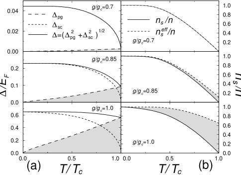
FIG. 1.: (a) Temperature dependence of the excitation gap $\Delta$, superconducting gap $|\Delta_{sc}|$ and pseudogap $\Delta_{pg}$ for coupling strengths $g/g_{c}=0.7$, $0.85$ and $1.0$. (b) Temperature dependence of the superfluid densities $n_{s}$ and $n_{s}^{\text{eff}}$ for the same coupling strengths as in (a). The shaded regions emphasize pseudogap effects.

Following the standard prescription for constructing the proper vertex correction corresponding to the superconducting self-energy [26] one obtains

$$\mathchoice{{\hbox{\boldmath$\displaystyle\delta\Lambda$}}}{{\hbox{\boldmath$\textstyle\delta\Lambda$}}}{{\hbox{\boldmath$\scriptstyle\delta\Lambda$}}}{{\hbox{\boldmath$\scriptscriptstyle\delta\Lambda$}}}_{sc}(K+Q,K)=\Delta_{sc}^{2}\varphi^{2}_{\mathchoice{{\hbox{\boldmath$\displaystyle k$}}}{{\hbox{\boldmath$\textstyle k$}}}{{\hbox{\boldmath$\scriptstyle k$}}}{{\hbox{\boldmath$\scriptscriptstyle k$}}}}G_{o}(-K-Q)G_{o}(K)\mathchoice{{\hbox{\boldmath$\displaystyle\lambda$}}}{{\hbox{\boldmath$\textstyle\lambda$}}}{{\hbox{\boldmath$\scriptstyle\lambda$}}}{{\hbox{\boldmath$\scriptscriptstyle\lambda$}}}(K+Q)\;.$$ (26)

Inserting Eqs. (8,12,26) into Eq. (25), after calculating the Matsubara sum, one arrives at

$$n_{s}=\frac{2}{3}\sum_{\mathchoice{{\hbox{\boldmath$\displaystyle k$}}}{{\hbox{\boldmath$\textstyle k$}}}{{\hbox{\boldmath$\scriptstyle k$}}}{{\hbox{\boldmath$\scriptscriptstyle k$}}}}\frac{\Delta_{sc}^{2}\,\varphi^{2}_{\mathchoice{{\hbox{\boldmath$\displaystyle k$}}}{{\hbox{\boldmath$\textstyle k$}}}{{\hbox{\boldmath$\scriptstyle k$}}}{{\hbox{\boldmath$\scriptscriptstyle k$}}}}}{E_{\mathchoice{{\hbox{\boldmath$\displaystyle k$}}}{{\hbox{\boldmath$\textstyle k$}}}{{\hbox{\boldmath$\scriptstyle k$}}}{{\hbox{\boldmath$\scriptscriptstyle k$}}}}^{2}}\left[\xi_{\mathchoice{{\hbox{\boldmath$\displaystyle k$}}}{{\hbox{\boldmath$\textstyle k$}}}{{\hbox{\boldmath$\scriptstyle k$}}}{{\hbox{\boldmath$\scriptscriptstyle k$}}}}(3-\varphi_{\mathchoice{{\hbox{\boldmath$\displaystyle k$}}}{{\hbox{\boldmath$\textstyle k$}}}{{\hbox{\boldmath$\scriptstyle k$}}}{{\hbox{\boldmath$\scriptscriptstyle k$}}}}^{2})+2\mu\right]\,\left[\frac{1-2\,f(E_{\mathchoice{{\hbox{\boldmath$\displaystyle k$}}}{{\hbox{\boldmath$\textstyle k$}}}{{\hbox{\boldmath$\scriptstyle k$}}}{{\hbox{\boldmath$\scriptscriptstyle k$}}}})}{2\,E_{\mathchoice{{\hbox{\boldmath$\displaystyle k$}}}{{\hbox{\boldmath$\textstyle k$}}}{{\hbox{\boldmath$\scriptstyle k$}}}{{\hbox{\boldmath$\scriptscriptstyle k$}}}}}+f^{\prime}(E_{\mathchoice{{\hbox{\boldmath$\displaystyle k$}}}{{\hbox{\boldmath$\textstyle k$}}}{{\hbox{\boldmath$\scriptstyle k$}}}{{\hbox{\boldmath$\scriptscriptstyle k$}}}})\right]\;.$$ (27)

We may write the superfluid density as $n_{s}=\Delta^{2}_{sc}\,F(\Delta)$ [where the form of the function $F$ can be obtained from Eq. (27)]. The same quantity corresponding to a BCS superconductor with effective gap parameter $\Delta$ is given by $n_{s}^{\text{eff}}=\Delta^{2}\,F(\Delta)$, so that, $n_{s}/n_{s}^{\text{eff}}=(\Delta_{sc}/\Delta)^{2}\leq 1$. In Fig. 1b we plot the temperature dependence of the normalized superfluid density $n_{s}/n$ (solid line) calculated from Eq. (27) for the same three representative values $g/g_{c}$ as above. These curves are compared (dashed line) with the quantity $n_{s}^{\text{eff}}/n$, which is a (BCS-like) function only of the excitation gap. For sufficiently weak coupling ($g/g_{c}\lesssim 0.7$) the two curves are indistinguishable. With increasing $g$ the separation between the two curves become evident, particularly in the vicinity of $T_{c}$, whereas at zero temperature there is no difference since $n_{s}=n$, independent of the coupling. This comparison thus demonstrates how different are these “pseudogap” superconductors. The superfluid density reflects most directly the temperature dependence of $\Delta_{sc}$, not the excitation gap.

The existence of residual pairing correlations below $T_{c}$ will affect thermodynamic properties as well. Indeed, upon analysis of data in underdoped cuprates, Loram et al [27] conjectured that the measured excitation gap squared can be expressed as the sum of the squares of a pseudogap and superconducting order parameter. This purely phenomenological analysis leads to a similar decomposition[28] of the excitation gap, as in Eq. (15) However, in contrast to the present work, these authors presumed that $\Delta_{pg}$ is temperature independent below $T_{c}$.

In summary, in this paper we have demonstrated that, if a pseudogap state arises from pairing correlations (fluctuations) above $T_{c}$, then these pairing fluctuations necessarily persist below $T_{c}$. These pseudogap systems are unconventional superconductors, in which pair fluctuations are present all the way down to the lowest temperatures. At $T=0$ these fluctuations (or $\Delta_{pg}$) vanish. A key manifestation of the “superconducting pseudogap” is in the nature of the excitation gap ($\Delta$), which differs significantly from the superconducting order parameter $\Delta_{sc}$, as $\Delta^{2}=\Delta_{sc}^{2}+\Delta_{pg}^{2}$. At a physical level we view $\Delta_{pg}$ as reflecting an additional energy associated with the attractive interaction, which must be overcome in order to create fermionic-like Bogoliubov quasi-particles. In this way, the excitations from the condensate in a BCS Bose-Einstein crossover theory can be viewed as intermediate between the (free) fermionic Bogoliubov quasi-particles of the BCS limit and the (bound) bosonic pairs in the Bose-Einstein regime. It should be stressed that our previous work on $d$-wave superconductors[19] reinforces the claim that the physics presented here for the $s$-wave case, is not qualitatively sensitive to the symmetry of the pairing interaction.

Experimentally, verification of this pseudogap scenario (for the underdoped cuprate superconductors) involves establishing the relation between $\Delta$ and $\Delta_{sc}$. Measurements of $n_{s}$ and $\Delta$ separately are possible (through penetration depth and ARPES experiments). Even more promising may be tunneling spectroscopy measurements of high $T_{c}$ superconductor-insulator-superconductor junctions in which the Josephson and quasiparticle current data can be simultaneously used to extract $\Delta$ and $\Delta_{sc}$.

We gratefully acknowledge useful discussions with A. Abrikosov, G. Mazenko, M. Norman and A. Zawadowski. This work was supported in part by the Science and Technology Center for Superconductivity founded by the National Science Foundation under award No. DMR91-20000.

REFERENCES

[1]
H. Ding et al, Nature 382 51 (1996).
[2]
A. G. Loeser et al, Science 273 325 (1996).
[3]
J. Loram et al, Phys. Rev. Lett. 71, 1740 (1993) and Physica C
235-240, 134 (1994).
[4]
W. W. Warren et al, Phys. Rev. Lett. 62, 1193 (1989).
[5]
V. Emery, S. A. Kivelson, Phys. Rev. Lett. 74, 3253 (1995); Nature 374 434 (1995).
[6]
P. A. Lee, N. Nagaosa, T. K. Ng and X.-G. Wen, Phys. Rev. B 57 6003
(1998) and references therein.
[7]
M. Randeria, (preprint, cond-mat/9710223), and references therein.
[8]
M. Randeria, in “Bose Einstein Condensation” edited by A. Griffin. D.
Snoke and S. Stringari (Cambridge Univ. Press, 1995), and references therein.
[9]
A. J. Leggett, J. Phys. (Paris) 41, C7 (1980); also in Modern Trends
in the Theory of Condensed Matter, edited by A. Pekalski and J. Przystawa,
Lecture Notes in Physics 115, Berlin (1980).
[10]
P. Nozières and S. Schmitt-Rink, J. Low Temp. Phys. 59, 195 (1985).
[11]
M. Randeria, J.-M. Duan, and L. Y. Shieh, Phys. Rev. Lett. 62, 981
(1989).
[12]
M. Randeria, N. Trivedi, A. Moreo, and R. T. Scalettar, Phys. Rev. Lett. 69, 2001 (1992).
[13]
C. A. R. Sa de Melo, M. Randeria, and J. R. Engelbrecht, Phys. Rev. Lett.
71, 3202 (1993).
[14]
R. Haussmann, Phys. Rev. B 49, 12975 (1994).
[15]
J. M. Serene, Phys. Rev. B. 40, 10873 (1989).
[16]
O. Tchernyshyov, Phys. Rev. B 56, 3372 (1997).
[17]
B. Janko, J. Maly and K. Levin, Phys. Rev. B 56, R 11 407(1997).
[18]
J. Maly, B. Janko, and K. Levin, (preprint,
cond-mat/9710187; 9805018).
[19]
Q. Chen et al., (preprint, cond-mat/9805032).
[20]
L. P. Kadanoff and P. C. Martin, Phys. Rev. 124, 670 (1961).
[21]
B. R. Patton, PhD Thesis, Cornell University, 1971 (unpublished); Phys. Rev.
Lett 27 1273 (1971).
[22]
D. Thouless, Ann. Phys. (NY) 10 553 (1960).
[23]
can be safely ignored for the purposes of calculating physical
quantities which involve only integrals over the self energy (e.g., ,
, etc.) but it must be retained for calculating spectral
functions, and densities of states, etc. Moreover, by including
in the self energy , its simple BCS form is
spoiled: the Bogoliubov quasiparticles acquire a finite lifetime.
[24]
Even if one takes into account the neglected
term, still remains negligibly small
compared to the total excitation gap at .
[25]
A. A. Abrikosov, L. P. Gor’kov, and I. E. Dzyaloshinski, Methods of
quantum field theory in statistical physics (Prentice-Hall, Englewood
Cliffs, N.J., 1963). We use the London gauge in our calculations of .
[26]
J. R. Schrieffer, Theory of Superconductivity, 3rd ed. (The
Benjamin/Cummings Publishing Company, Inc., Reading, Massachusetts, 1983).
[27]
J. W. Loram et al., J. Supercond. 7, 243 (1994).
[28]
J. W. Loram, K. A. Mirza, J. R. Cooper, and J. L. Tallon, Physica C 282-287, 1405 (1997). It should be stressed that these authors reach
different overall conclusions. They argue that the normal state gap results
from competing singlet correlations and not precursor superconducting
pairing, after having deduced the same decomposition of the excitation gap,
as we derive here.