Volume-collapse transitions in the rare earth metals

Abstract

We describe current experimental and theoretical understanding of the pressure-induced volume collapse transitions occurring in the early trivalent rare earth metals. General features of orbitally realistic mean-field based theories used to calculate these transitions are discussed. Potential deficiencies of these methods are assessed by comparing mean field and exact Quantum Monte Carlo solutions for the one-band Hubbard and two-band periodic Anderson lattice models. Relevant parameter regimes for these models are determined from local density constrained occupation calculations.

I INTRODUCTION

Many of the trivalent rare earth metals undergo a dramatic transformation in physical properties under compression, which is generally believed to arise from a change in the degree of $4f$ electron correlation [1, 2]. In some cases these changes appear abruptly across first-order phase transitions accompanied by unusually large volume collapses of 9 to 15%. Similar behavior is observed in the actinides, both for individual members under pressure, as well as across the series as a whole at atmospheric pressure [1]–[3]. Loosely speaking, the $f$ electrons act as if they participate in the crystal bonding in the compressed, more weakly correlated regime, and as if they do not at larger volumes where correlation effects are more dominant. The terms itinerant and localized, respectively, are commonly used to describe the differing $f$ electron behavior in these two regimes. The intuitive concepts underlying these terms permeate the extensive investigations of both series of $f$-electron metals [4, 5] .

Local density functional theory and its gradient approximation improvements appear to do well for the more weakly correlated phases at pressures above these transitions, as may be judged by the considerable success obtained for Ce and the light actinides [3, 6]. Comparable predictive capabilities are lacking in the more strongly correlated regime, as is a satisfactory treatment of the large-volume collapse phase transitions themselves.

It is the purpose of this paper to review current experimental and theoretical understanding of these transitions, with primary focus on efforts to develop a more rigorous and predictive treatment of strongly-correlated f-electron metals. One approach is the use of various corrected forms of local density functional theory which exhibit all-orbital realism, however, are still basically of a mean-field nature. General characteristics of these methods are described and compared to Hartree Fock. In order to assess correlation effects neglected by these methods, we report exact Quantum Monte Carlo (QMC) calculations for few-band effective Hamiltonians, and compare these to Hartree Fock results. In particular, new results are reported for the three-dimensional two-band periodic Anderson Hamiltonian, which represent a step towards using tera-scale computing resources to push QMC calculations into increasingly more realistic regimes.

In the remainder of this paper, Sec. 2 reviews the relevant experimental data as well as some of the simpler theoretical concepts suggested by this data. Section 3 provides parameter values which help place the rare earth transitions in the context of many-body effective Hamiltonians. Approximate but orbitally realistic theoretical approaches to understanding the transitions are discussed in Sec. 4, while results of exact Quantum Monte Carlo solutions for few-band effective Hamiltonians are presented and discussed in Sec. 5. Our summary is given in Sec. 6.

II BACKGROUND

This section reviews experimental data for the rare earth metals which characterize the issues of interest to this paper, as well as some of the associated calculations. Important results include the pressure-volume equations of state, sequences of structural phase transitions, variations in equilibrium volume across the series, and the magnetic moments. The primary focus here will be on the trivalent rare earths in the first half of the series, Ce ($f^{1}$), Pr ($f^{2}$), Nd ($f^{3}$), Pm ($f^{4}$), Sm ($f^{5}$), and Gd ($f^{7}$), excluding divalent Eu ($f^{6}$). In the course of this review, it is useful to simultaneously discuss simple one-electron concepts which help to organize these results. When viewed in this manner, one may interpret the data as showing evidence of $f$-electron participation in the crystal bonding in the higher-pressure more weakly correlated phases, whereas these manifestations appear largely absent in the lower-pressure more strongly correlated phases.

A Structural

Figure 1 shows the room temperature pressure-volume curves for Ce [7], Pr [8]–[11], Nd [12, 13], Pm [14], Sm

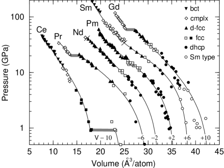
FIG. 1.: Pressure volume data for the rare earths. Structures are identified, with “cmplx” signifiying a number of complex, low-symmetry structures. The volume collapse transitions are marked by the wide hatched lines for Ce, Pr, and Gd, while lines perpendicular to the curves denote the d-fcc to hP3 symmetry change in Nd and Sm. The curves are guides to the eye. Note that the data and curves have been shifted in volume by the numbers (in ų/atom) shown at the bottom of the figure.

[15]–[17], and Gd [18, 19], where some of the more recent, higher-pressure data is plotted, with curves provided as guides to the eye. More complete references may be obtained elsewhere from recent papers dealing with systematics of the whole series [1, 2].  For clarity of presentation, the curves in Fig. 1 have been shifted in volume as shown at the bottom of the figure. The symbols change from open to filled or vice versa at structural phase transitions, which as may be seen are quite frequent. The volume changes at these phase transitions are generally a few percent or less. There are three notable exceptions which are marked with the thick hatched lines at 0.9 GPa in Ce (15% volume change) [7], 20 GPa in Pr (9%) [9]–[11], and 59 GPa in Gd (11%) [19].  These “volume-collapse” transitions demark the itinerant and localized regimes at pressures above and below the transitions, respectively, in these materials. Before discussing possible counterparts for the other three rare earths in Fig. 1, it is useful to first review common structural trends which will be identified with the localized regime.

The regular rare earths, those excepting Ce, Eu, and Yb, show a common structural sequence: hexagonal close packed (hcp) $\rightarrow$ Sm-type $\rightarrow$ double-hexagonal closed packed (dhcp) $\rightarrow$ face-centered cubic (fcc) $\rightarrow$ distorted fcc (d-fcc). The first four phases are all close packed and represent stacking variants of hexagonal layers such as the $ABC\cdots$ versus $AB\cdots$ order in fcc and hcp, respectively. There has been considerable discussion about the last phase [20]–[25], which was initially named distorted-fcc due to the appearance of superstructure reflections in the fcc diffraction pattern. The most recent opinion is that this phase is trigonal with eight atoms in the rhombohedral cell, and is due to a softening (TA) phonon at the $L$ point in the fcc Brillouin zone [23]–[25]. All or the latter part of this general hcp $\rightarrow$ Sm-type $\rightarrow$ dhcp $\rightarrow$ fcc $\rightarrow$ d-fcc sequence is observed under pressure in each of the regular rare earths. The valence electrons in these metals may be viewed as being compressed either by the application of pressure or by reducing the atomic number at fixed pressure [26]. Thus the lighter members of the series enter into the generalized sequence at successively later points, given their ambient, one atmosphere, room temperature phases: hcp (Gd), Sm-type (Sm), dhcp (Pm, Nd, Pr, and Ce). Aside from the lowest hcp and dhcp regions for Gd and Ce, respectively, which lie below the range plotted, the remaining phases in the general sequence may be seen in Fig. 1 for each of Pr–Gd, culminating in the high-pressure d-fcc end (filled up-triangles). While both Pr and Gd are seen to undergo the volume-collapse transition at room temperature from the d-fcc phase, recent work has shown this phase to disappear above a 573-K triple point in Pr, so that the Pr collapse above this temperature occurs directly from the fcc phase [11]. This behavior is similar to Ce, as seen in Fig. 1, which undergoes the collapse transition at room temperature from the fcc phase.

The significance of the regular rare earth sequence lies in the fact that it appears to have no connection whatsoever with $f$ electrons. An elegant demonstration of this fact is provided by the occurrence of this structural series, including the d-fcc phase [20], in compressed Y which has no nearby $f$ states at all [20, 27]. Theoretical calculations have furthermore demonstrated that the origin of the series lies in increased occupation of the $5d$ states caused by pressure-induced shift in the relative position of $6sp$ vs $5d$ bands [28]–[30].

The closed-packed and relatively high symmetry structures of the regular rare earth sequence stand in sharp contrast to the low symmetry structures seen at pressures just above the volume-collapse transitions in Pr (orthorhombic $\alpha$-U structure) and Gd (body-centered monoclinic), both represented in Fig. 1 by open diamonds. While the Ce volume-collapse is isostructural, fcc $\rightarrow$ fcc, at higher pressures in Fig. 1, one obtains a monoclinic or possibly the $\alpha$-U structure (open diamonds), which is a subject of current debate [31]. Beyond this, Ce transforms at 12 GPa into the body-centered tetragonal (bct) phase shown by the filled down-triangles in Fig. 1, a phase also assumed by Sm above 91 GPa and similarly denoted.

Low symmetry orthorhombic and monoclinic phases are of course prevalent among the early actinides, and have been demonstrated to arise from $5f$ electron participation in the bonding [6, 32]. Such phases are likewise taken to be evidence of itinerant $4f$ character in the high-pressure rare earths. However, it should be noted that for low $f$ band filling as well as for increasing pressure it is also possible to obtain higher-symmetry structures in the presence of $f$ electron bonding. The fcc structures of the collapsed $\alpha$-Ce phase as well as Th [33, 34] are characteristic of the $f^{1}$ metals, while high pressure bct phases are seen in Ce, Sm, Th, and predicted for U [6, 35]. Ultimately, U is predicted to reach an even higher symmetry bcc structure, as are a number of the other early actinides [6].

Finally, we turn to the three rare earths, Nd, Pm, and Sm, in Fig. 1 which do not appear to exhibit volume-collapse transitions. Recent experiments have identified Sm(V), indicated in Fig. 1 by the open diamonds, as a hexagonal phase with three atoms in the primitive cell (hP3). This is a rather unusual structure with open channels of roughly helical shape running along the $c$ direction, and an approximate fourfold coordination [2, 17]. An analysis of anomalies in the pressure-volume equation of state for Sm has led to the conclusion that a rapid increase of $4f$ bonding most likely begins with this phase [17]. Thus in the last part of the Sm sequence, d-fcc $\rightarrow$ hP3 $\rightarrow$ bct, the 91 GPa transition between d-fcc and hP3, marked by the line perpendicular to the $P$–$V$ curve in Fig. 1, is tentatively identified as the onset of itinerant $4f$ character in Sm. The same d-fcc $\rightarrow$ hP3 transition is seen in Nd [17], and is similarly marked in Fig. 1. Earlier work had noted a structural change in Nd at about 40 GPa, denoted by the open diamond in the figure [12, 13]. More recent measurements report the hP3 phase from 40 to 65 GPa in Nd, however do not publish pressure-volume data [17]. Data taken to date for Pm still falls within the regular rare earth sequence, as may be seen by the highest pressure d-fcc points in Fig. 1 (filled up-triangles), so it is not yet possible to speculate as to the onset of itinerant behavior in this material.

B Equilibrium volumes

Comparison of the atmospheric pressure or equilibrium volumes, $V_{0}$, of the $f$ and $d$ electron metals provides graphic evidence of regimes where the respective narrow-band electrons appear to be participating in the bonding or not, as has been appreciated for some years [3, 36]. Figure 2 shows these equilibrium volumes for the rare earths ($4f$), actinides ($5f$), and the $4d$ transition metal series [37]. The horizontal axis is band filling, $n/N$, i.e., the nominal number of $f$ or $d$ electrons divided by the shell capacity, $N=14$ or $10$, respectively.

Aside from the two divalent rare earths, the dependence of $V_{0}(n)$ for the rare earths is flat with a downward slope for increasing $n$ associated with the lanthanide contraction, i.e., the added $f$ electrons do not fully screen the valence electrons from the increased core charge. In contrast, the $4d$ transition series has a parabolic shape, which may be understood from simple tight-binding arguments [3]. Suppose the narrow band broadens symmetrically with compression about the atomic energy level,

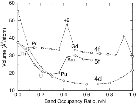
FIG. 2.: Atmospheric pressure volumes of the $4d$ transition metals, the rare earths ($4f$), and the actinides ($5f$). The two rare earths with large volumes are divalent.

and that it is characterized by a rectangular density of states, $D(\varepsilon)$, extending from $-W/2$ to $W/2$, as sketched in Fig. 3. The reduction in total energy, $\Delta E$, associated with having a finite band width and the corresponding pressure correction, $\Delta P$, is then

$$\Delta E = \int^{\mu}d\varepsilon\,\varepsilon\,D(\varepsilon)=-\frac{W}{2}\,\frac{n}{N}(N-n)\,,$$ (1)

$$\Delta P = -\frac{dE}{dV}=\frac{dW}{dV}\frac{n}{2N}(N-n)\,,$$ (2)

where $\mu$ is the Fermi energy. As the band width, $W$, grows with decreasing volume, $V$, Eq.(2) implies a negative contribution to the pressure which has a parabolic dependence on the band filling, $n(N-n)$. Such a dependence is clearly in evidence for the $4d$ transition metal series.

The actinides show mixed character as can be seen from Fig. 2. The first part of the series (Ac–Pu) exhibits similar parabolic dependence on band filling with increasingly lower values of $V_{0}$ suggestive of a $5f$ bonding contribution via Eq.(2). These same phases as already noted tend to exhibit complex low-symmetry structures also attributed to $5f$ bonding effects. The latter part of the series (Am and beyond), on the other hand, acts like a second rare earth series in which the bonding contribution, Eq.(2), no longer appears in evidence, and crystal

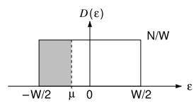
FIG. 3.: Schematic rectangular density of states of a band of width $W$ and capacity $N$, with $\mu$ the Fermi level.

structures are again of high symmetry [3].

While the present paper is concerned with the rare earth transitions, the pronounced similarities between the two series of $f$-electron metals serves to strengthen the combined understanding. In both cases the valence electrons may be effectively compressed either by the application of external pressure or by the reduction of atomic number at fixed pressure [26]. Thus the drop in volume from Am to Pu at ambient pressure is the volume-collapse in the actinides, which may therefore be viewed as occurring at negative pressures for the first five members (Th–Pu) of the series. The rare earth series is simply off-set in pressure, requiring the application of positive pressure to drive any of the rare earths through the collapse.

C Magnetic moments

Another key distinction between the localized and itinerant regimes appears to be the presence or absence, respectively, of magnetic moments on the $f$-electron sites. This is an especially important signature for theoretical simulations, since moment formation or loss is more amenable to study by simpler model calculations than is, for example, change in crystalline symmetry. Note that the loss of moment as detected by, e.g., magnetic susceptibility measurements may be due either to quenching of the $f$-shell moment itself or to its screening by the surrounding valence electrons. These two possibilities underly the Mott transition model of Johansson [38], and the Kondo volume collapse model of Allen and Martin [39] and Lavagna et. al. [40], for the rare earth collapse transitions, respectively. In both cases it is important to understand when the $f$-shell can support a stable moment. Simple one-electron concepts provide some insight into this issue, and are briefly discussed here after summarizing the experimental data.

The localized phases with magnetic moments generally undergo some kind of magnetic ordering transition at low temperatures, with Gd ($f^{7}$) having the highest ordering temperature at 293 K, followed by Tb ($f^{8}$) at 230 K among the rare earths [41], with the late actinides ordering at $\sim$50 K or below [42]. Since the room-temperature data in Figs. 1 and 2 is all in the respective paramagnetic regimes, the critical characteristic is the moment itself and not possible ordering, which we shall ignore in this paper. As well be seen later in discussing the exact Quantum Monte Carlo calculations, magnetic order can in fact be an unwanted distraction.

Figure 4 gives the observed atmospheric-pressure moments in the rare earth [41] and actinide [42] metals. The paramagnetic moments are extracted from the slope of the inverse magnetic susceptibility versus temperature in the paramagnetic regime, and may be compared to the corresponding free-ion values (solid line) given by

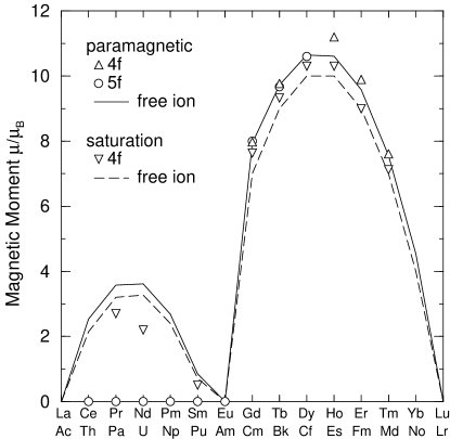
FIG. 4.: Atmospheric pressure magnetic moments of the rare earth and actinide metals (symbols), and simple free ion estimates (curves). Both paramagnetic and saturation moments are shown.

$g\,[J(J+1)]^{1/2}$. In the latter, one assumes Russel-Saunders coupling and takes the Hund’s rules ground state for each ion to obtain the total angular momentum, $J$, while $g$ is the Landé factor. Saturation moments are obtained either from the value of the magnetization at low temperature, or from extrapolations of magnetization data to infinite field. The corresponding free-ion value here is $gJ$ as plotted by the dashed line in Fig. 4.

It is evident from Fig. 4 that atoms in the late rare earth and actinide metals exhibit moments very close to their free ion values, which attests to $f$ electrons relatively unperturbed by their crystalline environment, consistent with localized $f$ electron behavior. The early actinides, Th–Pu, on the other hand, all exhibit temperature-independent paramagnetic susceptibility [42], consistent with the absence of magnetic moments. This is a dramatic change from free-ion behavior suggesting strong interaction between the $f$ electrons in these metals and their local environment. A temperature-independent paramagnetic susceptibility is also observed for Am [42], however, the $f^{6}$, $J\!=\!0$ ion should not have a moment even in the free ion limit, so that magnetic behavior is not particularly illuminating in this case.

The early rare earths are somewhat more complicated, since crystal field interactions split their Hund’s rules multiplets impacting their magnetic properties. The saturation moment of 2.7 $\mu_{\rm B}$ for Pr in Fig. 4 was obtained at 4.2 K [41], for example, while at a temperature on the order of the crystal field splitting, 40 mK, the size of the moment obtained from neutron scattering appears to be 0.36 $\mu_{\rm B}$ [43]. Nevertheless, these crystal field splittings are still rather small, so that the $2J\!+\!1$-level multiplet and its associated magnetic moment may be viewed as intact on the more coarse energy scale of interest to this paper. These crystal field interactions do serve as a reminder, however, of an approaching threshold beyond which the crystalline environment will destroy the local moments.

Simple one-electron concepts provide some understanding of the competing factors which determine whether an $f$-shell can support a stable moment. The Coulomb interaction, $\hat{I}$, within the manifold of $f$ states on a particular atomic site, $i$, may be written [44]

$$\hat{I}=\frac{1}{2}F^{0}\,\hat{n}_{if}\,(\hat{n}_{if}-1)+\mbox{\rm multipole terms}\,,$$ (3)

where $\hat{n}_{if}=\sum_{m\sigma}c_{ifm\sigma}^{\dagger}c_{ifm\sigma}$ is the total number operator for all 14 $f$ states indexed by $m\sigma$, and the monopole Slater integral, $F^{0}=U_{f}$, is the usual scalar Hubbard parameter describing the repulsion between each pair of $f$ electrons on the site. A Hartree-Fock expectation of the monopole part of Eq.(3) yields

$$\langle I\rangle_{0} = \frac{1}{2}F^{0}\,[(tr\,{\bf\rho}_{if})^{2}-tr\,{\bf\rho}_{if}^{2}]\,,$$ (4)

$$= \frac{1}{2}F^{0}n_{if}(n_{if}-1)+\frac{1}{2}F^{0}\sum_{\alpha}n_{i\alpha}(1-n_{i\alpha})\,,$$ (5)

where $n_{if}=tr\,{\bf\rho}_{if}$, and the $n_{i\alpha}$ are the eigenvalues of the $f\!f$ one-particle density matrix for the site $i$, ${\bf\rho}_{if}$, given by

$$({\bf\rho}_{if})_{m\sigma,m^{\prime}\sigma^{\prime}}\equiv\langle c^{\dagger}_{ifm\sigma}c_{ifm^{\prime}\sigma^{\prime}}\rangle\,.$$ (6)

It is the second term in Eq.(5) which is interesting, as it is minimized by having “sharp” orbital occupations, $n_{i\alpha}=0$ or 1. This is achieved in Hartree-Fock by one-electron energies, $\epsilon_{{\bf k}\alpha}$, containing the term $U_{f}(n_{f}-n_{\alpha})$, where $n_{f}$ and $n_{\alpha}$ are site-independent values of $n_{if}$ and $n_{i\alpha}$, respectively. This term discriminates between occupied and empty states, placing the latter higher by $U_{f}$ when the $n_{\alpha}=0,1$. The multipole terms in Eq.(3) supplement Eq.(5) in impacting the nature of the orbitals which diagonalize the $f\!f$ density matrix, ${\bf\rho}$, as well as helping to select those which will be populated. The exchange terms, for example, favor all parallel spins for $n_{if}\!\leq\!7$ (Hund’s first rule). Other multipole terms seek to maximize the total angular momentum for the $f$ shell (second rule), or an approximation to this in mean field. The net effect in the exact (with intraatomic correlations) solution is of course to build large values of the total spin, $S_{if}$, and total angular momentum, $L_{if}$, from the multi-$f$-electron shell, which may then be combined by spin-orbit (third rule) into a total moment $gJ$.

This behavior is in contrast with the one-electron bonding effect in Eq.(1), where to a rough approximation one can find all spin and orbital types in the lower part of the band. This follows from the fact that the overall size of the one-body, intersite hopping matrix elements, $\langle\phi_{iflm}|H|\phi_{jflm^{\prime}}\rangle$, is set by the tail of the radial wavefunction which to first approximation is independent of $m$, and that geometric effects on these matrix elements tend to be smeared out both by the variety of neighboring atom positions as well as by the range of phase relations associated with points throughout the Brillouin zone. As a consequence, the band broadening mechanism of Eq.(1) is relatively indiscriminate in terms of spin-orbital occupations, favoring roughly $n_{i\alpha}\sim n_{if}/14$ which serves to quench spin and orbital moments.

It seems clear in the extremes $W_{f}>>U_{f}$ and $W_{f}<<U_{f}$ that the competition between Eqs.(1) and (3) results in the absence or presence of a moment, respectively. It is also evident how at least Hartree-Fock goes about reducing the $f$ bonding effect of Eq.(1) in the latter regime, by splitting the occupied and empty states to create a new entirely full band for which $n(N-n)\!=\!0$. The major current debate concerns how the experimentally observed moment is actually first lost with increasing pressure (or $W_{f}/U_{f}$) for the $4f$ and $5f$ metals, whether the $f$ moment is first quenched similar to the manner discussed here and by the Mott transition model [38], or whether while still in a robust state it is first screened away by a surrounding cloud of valence electrons as in the Kondo volume collapse model [39, 40].

III PARAMETERS

To provide contact with the intuitive concepts discussed in the previous section as well as to motivate model problems which can be exactly solved by Quantum Monte Carlo techniques, it is useful to characterize the rare earth metals in terms of the effective Coulomb repulsion between $f$ electrons on the same site, $U_{f}$, the position of the $f$ level, $\varepsilon_{f}$, and the $f$–$f$ and $f$–valence hopping interactions, $t_{f\!f}$ and $t_{fv}$, or the equivalent expressions in band widths, $W_{f\!f}$ and $W_{fv}$, respectively. These results were obtained as a function of compression for fcc phases of the rare earths using a scalar-relativistic linear muffin-tin orbitals (LMTO) method in the atomic-sphere approximation plus combined correction [45, 46]. All electrons were treated self consistently. The specific approximations used to calculate the different parameters have been discussed at length elsewhere [44, 47, 48]. While not rigorous, they are reasonable, and known to give values of the Coulomb interactions and hopping parameters within $\sim 20$% of values deduced from experiment in other materials [44, 47, 48].

The monopole contribution to the $f$–$f$ Coulomb interaction, $U_{f}$, and the site energy, $\varepsilon_{f}$, may be obtained from self-consistent calculations of the total energy, $E(n)$, or the $f$-orbital eigenvalue, $\lambda_{f}(n)=dE(n)/dn$, as a function of $f$ occupation, $n$. Although more sophisticated methods exist for decoupling the orbitals so as to control their occupations [48], the $4f$ orbitals are sufficiently well localized in the present materials that we have simply treated them as part of the self-consistent core [47]. The formal definition of $U_{f}$ is

$$U_{f} = E(n_{f}\!+\!1)+E(n_{f}\!-\!1)-2E(n_{f})\,,$$ (7)

$$\approx \lambda_{f}(n_{f}\!+\!\mbox{$\frac{1}{2}$})-\lambda_{f}(n_{f}\!-\!\mbox{$\frac{1}{2}$})\,,$$ (8)

while the site energy, $\varepsilon_{f}$, may be defined in terms of the removal energy, $E(n_{f})-E(n_{f}\!-\!1)$,

$$\varepsilon_{f}+U_{f}(n_{f}\!-\!1) \approx E(n_{f})-E(n_{f}\!-\!1)$$ (9)

$$\approx \lambda_{f}(n_{f}\!-\!\mbox{$\frac{1}{2}$})\,.$$ (10)

These equations provide the best quadratic approximation, $E_{0}+\varepsilon_{f}n+U_{f}n(n-1)/2$, to $E(n)$ in the vicinity of the nominal integer occupation, $n\!=\!n_{f}$. In principle one should probe the dependence on occupation of only a single $f$ site in the infinite solid. For metals, however, the screening is so effective that one may in practice alter the occupation at every site. This requires use of a neutralizing electrostatic background, or exchanging the electrons between the $f$ site and the valence band Fermi level, $\mu$. In the latter case, case $-\mu$ should be added to the left side of Eq.(9).

Figure 5 shows $U_{f}$ versus atomic volume for the five rare earth metals which have exhibited anomalies under pressure. The pluses mark the boundaries of the volume collapse transitions (Ce, Pr, Gd) or the d-fcc $\rightarrow$ hP3 symmetry change (Nd, Sm). The open squares are the atmospheric-pressure values calculated by Herbst and Wilkins [49], however, omitting their correlation and Hund’s rules corrections to be consistent with the present work. These corrections to $U_{f}$ are less than 1 eV for Ce,

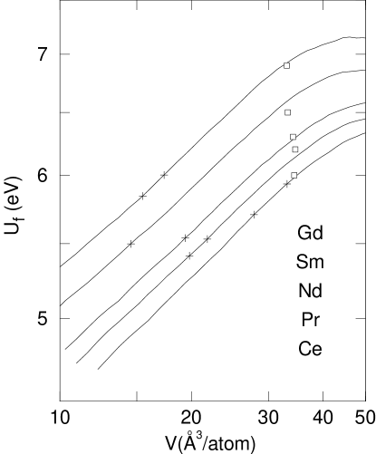
FIG. 5.: Calculated Coulomb interaction, $U_{f}$, for the rare earth metals as a function of volume.

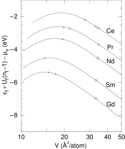
FIG. 6.: Calculated removal energy, $\varepsilon_{f}+U_{f}(n_{f}\!-\!1)$, relative to the valence Fermi energy, $\mu_{v}$, for the rare earth metals as a function of volume. $n_{f}$ is the nominal integer $f$ occupation.

Pr, Nd, and Sm, however, increase the Gd value by 5.4 eV. With the corrections, Herbst and Wilkins found quite good agreement with electron spectroscopy data [49]. The general trends evident in Fig. 5 are as expected. The heavier rare earths have more narrow $4f$ bands, reflecting more compact orbitals, and therefore exhibit larger values of $U_{f}$. In all cases the effect of compression is to enhance screening and therefore reduce $U_{f}$. In the range of interest these reductions are $\sim 20$%.

The removal energies, $E(n_{f})-E(n_{f}\!-\!1)\approx\varepsilon_{f}+U_{f}(n_{f}\!-\!1)$, are shown in Fig. 6 relative to the Fermi energy, $\mu_{v}$, of the three valence electrons per site. As before, the pluses mark the location of the anomalies, while the open circles simply locate the atmospheric-pressure volumes. The comparable values of Herbst and Wilkins [49] (absent correlation and Hund’s rules corrections) show about the same dependence on atomic number, however, are $\sim 2$ eV higher in energy than the present results. Their correlation and Hund corrections then lower these values by 1–3 eV for Ce–Sm (4.6 eV for Gd), so that their final results are within about an eV of the uncorrected values in Fig. 6 for Ce–Sm. Herbst and Wilkins found the same characteristic volume dependence as also seen here. In particular, the maxima seen in Fig. 6 in the range 15–20 ų/atom corresponds to the end of an electronic $s$–$d$ transition caused by the rising $6sp$ levels dumping their electrons into the $5d$ states. As they note, the shifting balance of kinetic and potential energies under compression will eventually cause the $5d$ band to move upward relative to $4f$ states, as seen at the lower volumes. The

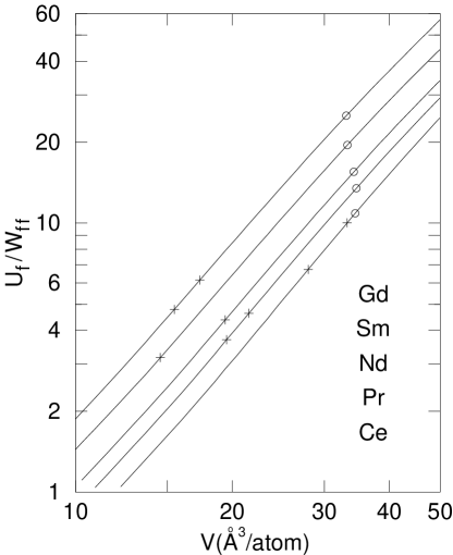
FIG. 7.: Calculated ratio, $U_{f}/W_{f\!f}$, where $W_{f\!f}$ is the $f$ band width due to $f$–$f$ hybridization, for the rare earth metals as a function of volume. These results were obtained for an fcc lattice, so that near-neighbor hopping interactions, $t$, may be estimated by dividing the corresponding band widths by 16.

important conclusion to draw from Fig. 6, is that the $4f$ levels are rising as a function of compression throughout the range leading up to the pressure anomalies.

The contribution to the $4f$ band width due to $ff$ hopping interactions may be simply determined by the width of the pure $f$ Wigner-Seitz band, which is given by the energy difference between $f$ orbitals whose logarithmic derivatives at the atomic-sphere boundary are 0 (band bottom) and infinite (band top), respectively. The $4f$ band widths, $W_{f\!f}$, obtained in this way for the five rare earths are plotted in Fig. 7 in the ratio $U_{f}/W_{f\!f}$ as a function of volume. As before, circles and pluses mark values at the atmospheric-pressure and the transition volumes, respectively. The heavier rare earths may be expected to have both narrower $f$ bands and larger Coulomb interactions, leading to the ordering shown. The functions $U_{f}$, $W_{f\!f}^{-1}$, and $U_{f}/W_{f\!f}$ depend on the 0.2, 2.0, and 2.2 powers of volume in compression, to within about $\pm 0.05$ in these exponents. Canonical band arguments suggest a $d^{-l-l^{\prime}-1}$ dependence for the overlap of $l$ and $l^{\prime}$ orbitals a distance, $d$, apart [45, 46], or $W_{f\!f}^{-1}\sim V^{2.3}$, which is close to what is observed here.

The width in energy over which $f$ states are spread also arises from $f$-valence hopping interactions or hybridization. We have obtained root-mean-square widths, $W^{\,\rm rms}$,

$$W^{\,\rm rms}=\left[\int d\varepsilon\,D_{f}(\varepsilon)(\varepsilon-\bar{\varepsilon})^{2}/\int d\varepsilon\,D_{f}(\varepsilon)\right]^{1/2}\,,$$ (11)

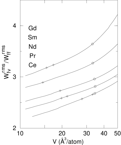
FIG. 8.: Calculated ratio, $W^{\,\rm rms}_{fv}/W^{\,\rm mrs}_{f\!f}$, for the rare earth metals as a function of volume. Here, $W^{\,\rm rms}_{f\!f}$ and $W^{\,\rm rms}_{fv}$ are the rms $f$ band widths due to $f$–$f$ and $f$–valence hybridization, respectively.

using $f$ partial densities of states, $D_{f}(\varepsilon)$, obtained in three ways. In one case we have taken the orthogonalized one-electron Hamiltonian matrices obtained from the self-consistent one-electron potentials and set all $f$-valence matrix elements to zero, so that the resultant band width, $W^{\,\rm rms}_{f\!f}$, is due predominantly to $ff$ interactions with some small crystal field contributions. In the second case, we replace the $ff$ blocks by the identity matrix times the average $f$ energy, obtaining a width, $W^{\,\rm rms}_{fv}$, due to $f$-valence interactions. In the third case, we have used the unmodified orthogonalized Hamiltonian matrices, obtaining the full $f$ width, $W^{\,\rm rms}_{f}$. Note that it is rigorously the case for these rms widths that

$$W^{\,\rm rms}_{f}=[\,(W^{\,\rm rms}_{f\!f})^{2}+(W^{\,\rm rms}_{fv})^{2}\,]^{1/2}\,.$$ (12)

The ratios, $W^{\,\rm rms}_{fv}/W^{\,\rm rms}_{f\!f}$, are shown in Fig. 8 for the five rare earths. In compression they depend on the 0.16 power of the volume to within $\pm 0.06$ in the power. If the $f$–$f$ overlap acts like $l\sim 2.5$ in its $d^{-l-l^{\prime}-1}$ dependence ($W_{f\!f}\sim V^{-2.0}$), then the volume dependence of the ratio in Fig. 8 suggests a valence $l\sim 2$. This is consistent with the general belief that the important intersite $f$-valence hybridization is with $d$ states.

The implication of Fig. 8 is that $f$-valence hybridization is a more important contributor to the overall $f$ band width in the rare earths than is direct $f$–$f$ hybridization. Earlier work suggested comparable impact, based on the boundaries of one-electron bands of $f$ symmetry [50]. Equation (11), however, also measures $f$ orbital admixtures which can occur farther out in energy as parts of bands identified by symmetry as of other $l$ character.

If we define $W_{fv}\equiv W_{f\!f}\,W^{\,\rm rms}_{fv}/W^{\,\rm rms}_{f\!f}$, then Figs. 5–8 imply that the rare earth collapse transitions (or symmetry changes in Nd and Sm) occur over the ranges $U_{f}/W_{fv}=$ 3.7–2.6 (Ce), 1.8–1.5 (Pr), 1.6 (Nd), 1.1 (Sm), and 1.9–1.5 (Gd). These ratios are all in the range 1–2 except for $f^{1}$ Ce, which has the lowest band filling. If the combined $f$ band width, $W_{f}$, is given by an expression such as Eq.(12), then the corresponding values for $U_{f}/W_{f}$ would be reduced by 5%–7%.

To make contact between the parameters presented in this section and the models to be discussed in Sec. 5, note that for near-neighbor interactions and only $t_{f\!f}$ hopping, the full $f$ band width, $W_{f}=W_{f\!f}$, is $16\,t_{f\!f}$ for the fcc structure used in Fig. 7 while $12\,t_{f\!f}$ for the simple cubic structure assumed in Sec. 5. As a matter of convenience, and to acknowledge the scaling in Eq.(12), we shall also define the width $W_{f}=W_{fv}\equiv 12\,t_{fv}$ for the simple-cubic two-band periodic Anderson model calculations in Sec. 5 with a dispersionless ($t_{f\!f}\!=\!0$) $f$ band.

IV MODIFIED MEAN FIELD THEORIES

It is generally believed that the volume collapse transitions also occur at zero temperature, in which case they should in principle be reproduced by density functional theory [51] as properties of the ground state total energy. In practice, however, local density functional (LDF) theory, which resembles a modified Hartree mean field [52], does not give the transitions. There has been much effort to find improvements which are more successful in this regard. These include the use of spin [53]–[56] and orbital [57, 58] polarization, self-interaction corrections [58]– [61], and the LDA+U method [62]. A critical comparison of these methods has been given recently for the related problem of transition metal monoxides [63]. Here, we briefly review such calculations for the $f$ electron metals. Then we describe results of screened Hartree-Fock calculations on orbitally realistic effective Hamiltonians which are similar to some of these methods, and by this means illustrate a number of common features of the modified mean field theories.

A Corrected local density functional theory

One of the most successful applications of spin-polarized LDF theory was to the actinides, in which the jump in equilibrium volumes seen in Fig. 2 was reproduced [53], as well as the delocalization transition in compressed Am [54]. Similar calculations for compressed Ce [55] and Pr [56] were less successful, with too little of the $f$ bonding contribution removed in the large volume spin-polarized region. Note that the collapse between Pu and Am in Fig. 2 occurs near half filling of the $5f$ shell so that spin polarization potentially reduces $n(N\!-\!n)$ in Eq.(2) by a factor of eight for Am, in contrast to only about a factor of two for the early rare earths, Ce and Pr.

The solution to this difficulty has been orbital polarization [57], in which a term proportional to the square of the $z$ component of the total angular momentum is added into the total energy functional so as to simulate Hund’s second rule. Combined with spin polarization, the resulting calculations discriminate amongst the 14 $f$ states in favor of large values of the $z$ components of total spin, $M_{S}$, and angular momentum, $M_{L}$, for the $f$ shell. Both effects arise from the multipole terms in Eq.(3), and their size is dictated by combinations of the material specific values of Slater’s $F^{2}$, $F^{4}$, and $F^{6}$ integrals. The consequence is the possibility of splitting off occupied bands of any integral number of $f$ electrons per site, i.e., reducing $n(N\!-\!n)$ to potentially zero for any value of $n$. Such calculations for the collapse transitions in Ce [57] and Pr [58] have yielded reasonably good agreement with experiment, in the latter case supplemented also by generalized gradient corrections to the exchange-correlation potential. Plots of the spin and orbital polarization in the first case show roughly maximal values in the localized regime, which decay to zero in the vicinity of the transition [57].

One may also discriminate amongst the 14 $f$ orbitals purely on the basis of their occupation, as noted in regard to the second term in Eq.(5), with the size of the effect given by the monopole integral, $F^{0}$, the familiar Hubbard $U_{f}$. Because of the poorly cancelled self-interaction of an electron with itself in LDF theory as well as its spin and orbitally polarized generalizations, this effect is largely absent from the above calculations. It may be reintroduced by performing self-interaction corrected (SIC) LDF calculations generally combined with spin polarization. Such calculations split the occupied and empty $f$ states, determined self-consistently, by $U_{f}$ and therefore also serve to reduce $n(N\!-\!n)$ of Eq. (2) potentially to zero, for any value of $n$, in the large volume localized regime. Quite satisfactory results have been obtained for both the Ce [59]–[61] and Pr [58] volume collapse transitions. The LDA+U method [64] is an ad hoc way of achieving the same end in a much easier calculation by simply adding the second term in Eq.(5) to the LDF-total energy functional. Apparently, a value of $U_{f}\sim 3$ eV, about half of what would be expected, is required to make the Ce transition occur in the right place [62]. This is interesting, since judging from the separations between the centers of gravity of the empty and occupied $4f$ states, SIC calculations for Ce [59] and Pr [65] both correspond to $U_{f}\sim 9$–10 eV. It might also be noted that $\sim$40% smaller effective $U$ values are also required in analytic random phase and conserving approximations when attempting to fit exact Quantum Monte Carlo results [66].

B Hartree Fock with static screening

The Hartree-Fock (HF) method has no self interaction problem. Unfortunately, its electron-electron interactions are unscreened so that the one-electron spectrum reflects the full value of the bare Slater monopole integrals, e.g., $F^{0}\sim 26$ eV for the $4f$ states in Ce [67, 68]. If the Hamiltonian is written in second quantized form, however, it is trivial to replace $F^{0}$ by a screened value. HF solution of such a Hamiltonian includes some correlation effects via this static screening, and might be viewed as a further approximation to the GW method [69] .

We report here such Hartree-Fock calculations for the Hamiltonian,

$$H= \sum_{{\bf k},\alpha,\beta}h_{\alpha\beta}^{\rm LDF}({\bf k})\,c^{\dagger}_{{\bf k}\alpha}c_{{\bf k}\beta}\;+\;\sum_{{\bf k},m,\sigma}(\varepsilon_{f}-\varepsilon_{f}^{\rm LDF})\,c^{\dagger}_{{\bf k}fm\sigma}c_{{\bf k}fm\sigma}$$ (14)

$$+\;\frac{1}{2}U_{f}\sum_{i}\hat{n}_{if}(\hat{n}_{if}-1)\,,$$

where ${\bf k}$ are vectors in the Brillouin zone, $\alpha\equiv lm\sigma$ represents the usual angular, magnetic, and spin quantum numbers, $i$ are the lattice sites, and $\hat{n}_{if}=\sum_{m\sigma}c^{\dagger}_{ifm\sigma}c_{ifm\sigma}$ is the total $f$ number operator for site $i$. We consider only one atom per unit cell, so that the localized HF solutions of Eq.(14) will be ferromagnetic. Rather than the limited hopping parameter information given in Figs. 7–8, we use the full, converged, ${\bf k}$-dependent LDF Hamiltonians, $h^{\rm LDF}_{\alpha\beta}({\bf k})$, which are 32$\times$32 matrices ($s$–$f$ basis plus spin) that have been orthogonalized. They are corrected by replacing the LDF $f$ site energy by its constrained occupation counterpart from Fig. 6, and adding the screened, $f$–$f$ monopole Coulomb interaction, though as yet, no multipole contributions such as exchange. Note that each of $h^{\rm LDF}$, $\varepsilon^{\rm LDF}_{f}$, $\varepsilon_{f}$, and $U_{f}$ is volume and material dependent.

Figure 9 summarizes the ground state HF solutions of Eq.(14) for Ce. We have omitted the spin-orbit interaction here for simplicity, however, we obtain similar results with this interaction added to Eq.(14). The figure shows the total $f$ occupancy per site, $n_{f}\!=\!n_{if}\!\equiv\!\langle\hat{n}_{if}\rangle$ as a function of position of the $f$ level, $\varepsilon_{f}$, relative to the valence Fermi level, $\mu_{v}$, i.e. that for just three $spd$ electrons per site. Each curve corresponds to a different volume. The calculated values of $\varepsilon_{f}\!-\!\mu_{v}$ from Fig. 6 are shown as the open circles on the appropriate curves. The use of $\varepsilon_{f}$ as an independent variable here is both instructive and offers some sense of the impact of the $\sim 1$ eV uncertainty in these values discussed in Sec. 3.

Note first that at large volume (solid curve, $V\!=\!56.7\,$ų/atom), where the hybridization interactions are weak, one obtains a staircase structure of integer values for $n_{f}$. As $\varepsilon_{f}$ drops below $\mu_{v}$, only one $f$ electron state

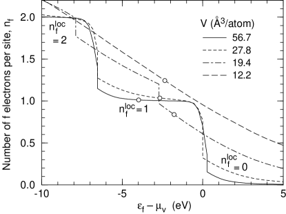
FIG. 9.: Static-screened Hartree-Fock calculations for Ce. The number of $f$ electrons per site, $n_{f}$, is shown as a function of the $f$ level position, $\varepsilon_{f}$, relative to the valence Fermi energy, $\mu_{v}$, at four different volumes. The calculated values of $\varepsilon_{f}$ from Fig. 6 are shown by the open circles. The solutions exhibit different branches characterized by integer numbers, $n_{f}^{\rm loc}$, of occupied split-off $f$ bands.

is occupied at first due to the cost, $U_{f}$, for adding a second. Only when $\varepsilon_{f}$ is lowered an additional $U_{f}$ below $\mu_{v}$ is the second $f$ electron picked up, and so on. Such a plot is similar to an integral over the $f$-decomposed density of states, so that the plateaus correspond to Mott-like gaps in the $f$ spectrum. A related plot, where the chemical potential is varied, is a standard tool used in analyzing the results of many-body simulations [70]. This staircase structure is smeared out with the increasing hybridization width of the $f$ band as volume is reduced. When this width becomes so large that $U_{f}$ is effectively unimportant, $n_{f}$ grows linearly with decreasing $\varepsilon_{f}\!-\!\mu_{v}$. The idealized limits of localized and itinerant character are associated with such staircase versus linear behavior, respectively. The usefulness of a plot such as Fig. 9 is that it provides a visual sense of where a given material at a specific volume lies between these two limits. In particular, the short dashed curve in Fig. 9 corresponds to a volume very close to that of the collapsed $\alpha$ phase of Ce, suggesting that the Ce transition lies closer to the localized limit. The ratios $U_{f}/W_{ff}=6.7$ and $U_{f}/W_{fv}=2.6$ from Figs. 7–8 for Ce at the $\alpha$ volume are consistent with this observation, and might be compared to 3–5 and 1.1–1.5, respectively, on the low-volume side of the other rare earth transitions.

We have labeled the HF solutions in Fig. 9 by integer values of $n_{f}^{\rm loc}$, referring to the number of $f$ electrons split off in low energy fully occupied bands. The partial $f$ density of states (DOS) shown in Fig. 10 illustrates the differences at essentially the $\alpha$-Ce conditions ($V\!=\!27.8$ ų/atom and $\varepsilon_{f}\!-\!\mu_{v}=-2.2$ eV). The ground state $n_{f}^{\rm loc}\!=1$ solution (dashed/shaded curve) exhibits the features associated with one localized electron: 98% occupancy of a single spin-orbital (total $n_{f}\!=\!1.05$), and a separation

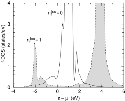
FIG. 10.: Ce $f$ densities of states for stable $n_{f}^{\rm loc}\!=\!1$ and metastable $n_{f}^{\rm loc}\!=\!0$ Hartree-Fock solutions for Ce at essentially the $\alpha$ phase volume and $\varepsilon_{f}$. The zero of energy is the full system Fermi energy, $\mu$.

between occupied and empty $f$ states of $\sim U_{f}\!=\!6.7$ eV. The metastable $n_{f}^{\rm loc}\!=0$ solution, on the other hand, has its $n_{f}\!=\!0.71$ $f$ electrons distributed across all of 14 $f$ states, and is consistent with itinerant $f$ electron behavior. While one might have expected the latter solution to have the lower energy, Sandalov et. al. [62] have found a similar result in their tight-binding and LDA+U calculations, observing that they would need to reduce $U_{f}$ to $\sim\!2.7$ eV to put the itinerant state lower.

While it occurs at too high compression, Fig. 9 does ultimately predict a transition in Ce, since the boundary between $n_{f}^{\rm loc}\!=\!1$ and 0 solutions shifts to lower values of $\varepsilon_{f}\!-\!\mu_{v}$ with compression. The open circle for $V\!=\!19.4$ ų/atom (dash-dot curve) may be seen to lie on the $n_{f}^{\rm loc}\!=\!0$ branch. We find the same behavior in compressed Pr however, the analogous transition is from $n_{f}^{\rm loc}\!=\!2$ to 1, as if the two $f$ electrons in Pr delocalize one at a time in the present calculations.

The present HF results could be improved by including multipole terms and, as noted by Sandalov et. al. [62], by using state-dependent hopping interactions. Nonetheless, the present results illustrate some features which appear to be characteristic of the modified mean-field theories as a class. In all cases these theories model the localized regime by polarized solutions with an integer number, $n^{\rm loc}_{f}$, of filled split-off bands of relatively select spin-orbital character. The pressure induced transitions predicted by these methods involve a shift of these bands to the vicinity of the Fermi level, i.e., a transfer of spectral weight in roughly integer units of electrons per atom. Moreover, these transitions are abrupt in the sense that there are generally two distinct solutions (e.g., Fig. 10) with total energies which cross at some point. To anticipate the next section, correlation effects enable a more continuous and nonintegral transfer of $f$ spectral weight from the low-lying localized or polarized $f$ states to higher energies [71]. In the case of Ce, however, Svane [61] has claimed that such effects modify the total energy in the vicinity of the crossing, but not further away where the Maxwell common-tangent touches the two energy curves.

V EXACT QUANTUM MONTE CARLO CALCULATIONS

As emphasized above, electronic correlations play an important role in volume collapse transitions, yet approximate mean-field treatments of their effects, such as Hartree-Fock theory, suffer serious deficiencies. We therefore turn to an approach, Quantum Monte Carlo (QMC), which can treat electron–electron interactions exactly. QMC is computationally very expensive, and while models of increasingly accurate orbital realism can now be simulated, it is still not feasible to study a system with the full complexity of, for example, Ce. A crucial task is to put together LDF calculations which do treat the full electronic structure, with a QMC treatment of simpler Hamiltonians which can focus on the physics missed by LDF theory.

A Quantum Monte Carlo method

The idea of QMC is to use an exact mathematical transformation to rewrite the interactions between two electrons as a coupling of a single electron with a classical fluctuating field, which then mediates the interactions indirectly. The resulting single–particle quantum mechanical problem can be solved, leaving only an integration over all possible values of the classical field. This integration is in an extremely high dimensional space. For every pair of interacting orbitals in the original Hamiltonian, there are $L$ auxiliary field variables, where $L$ is roughly the ratio of the bandwidth to the temperature. Such high dimensional integrals can be done by classical monte carlo methods.

This formalism is straightforward and exact, but there are a number of difficulties in its implementation. The first is the scaling of the computation time with system size. While the integral to be done is classical, the integrand is non–local. Each field variable interacts with all the others, not just with a few “neighbors”. To update every component of the field takes a computation time which scales as the cube of the number of orbitals. Thus to change the number of orbitals per site from a Hamiltonian with one conduction and one local orbital per site, to a fully realistic all–orbital description in which 16 orbitals are retained, increases the computational expense by a factor of $8^{3}$.

Going to lower temperatures also involves increased effort, since the number of field variables scales as bandwidth over temperature. This is only a linear cost. That is, to double $\beta=1/T$ only doubles the cpu requirements. However, a more serious difficulty is also encountered. In many situations the integrand, which one is using as a sampling probability, can go negative. When this occurs, QMC simulations are no longer feasible. This “sign problem” does not occur for certain “symmetric” choices of the parameters in the Hamiltonian, and also does not occur at high temperatures. Nevertheless, it is a significant limitation to the fillings and interaction strengths for QMC in general.

The state–of–the–art in QMC on vector supercomputers are simulations of Hamiltonians with roughly a hundred orbitals. This means periodic lattices of, for example, 4x4, 6x6, 8x8, and 10x10 for a two dimensional single orbital model, and 4x4, 6x6, and 8x8 for a two dimensional two orbital model [72, 73, 74]. Such sets allow for extrapolations to the thermodynamic limit, particularly when the form of the finite size correction is known [75, 76]. It is clear that simulations with increased orbital realism, in three dimensions, require significantly more powerful hardware, such as is now becoming available with the parallel platforms. QMC is ideally suited for parallelization; it achieves an almost linear speedup as more and more processors are applied to a problem. We will discuss finite size effects in more detail later, but for the moment let us say that we do not expect them to be too significant for the thermodynamics, since the energy involves only local quantities [78]. Therefore our work will focus on the issue of more orbitals per site, as opposed to increased spatial size. This is also the direction desired for increased contact with LDF theory.

B The Hubbard and Anderson Lattice Hamiltonians

The determinant Quantum Monte Carlo calculations we will use consider electrons which move on a discrete lattice of atomic sites, and their associated orbitals [77]. Continuum QMC methods, like Green’s Function Monte Carlo, do exist, but as yet appear less easily applied to the problems of magnetic moment formation, magnetic ordering, and singlet formation, which are relevant to the volume collapse transition. The simplest lattice model which might be applied to the present system is the single–band “Hubbard Hamiltonian.” Originally formulated for “d” electron systems, in the present case one might consider a single effective $f$ electron. If we denote by $f_{i\sigma}^{\dagger}$ an operator which creates such an electron on site $i$ with spin $\sigma$, then this Hamiltonian may be written

$$H = -t_{ff}\sum_{\langle ij\rangle\sigma}(f_{i\sigma}^{\dagger}f_{j\sigma}+f_{j\sigma}^{\dagger}f_{i\sigma})$$ (16)

$$+U_{f}\sum_{i}(n_{i\uparrow}-\frac{1}{2})(n_{i\downarrow}-\frac{1}{2})-\mu\sum_{i\sigma}n_{i\sigma}\,.$$

The kinetic energy and interactions in this model are as local as possible, hopping between near–neighbor sites $\langle ij\rangle$ only, and interactions between the density of electrons, $n_{i\sigma}=f_{i\sigma}^{\dagger}f_{i\sigma}$, only on the same site. The interaction term has been written in a special form which makes “half–filling,” a density of one electron per site on average, occur precisely at $\mu=0$ for any choice of temperature $T$ or parameters $t_{ff},U_{f}$ in the Hamiltonian. Furthermore there is no sign problem. These desirable properties require a bipartite lattice, composed of two sublattices, such that all near neighbors of an atom on one sublattice lie on the other. Body-centered cubic and simple cubic are examples, however, face-centered cubic is not. Since, for near-neighbor interactions, the first structure has a divergent noninteracting density of states at $\mu=0$, the present simulations have considered the simple cubic structure.

The kinetic energy term in Eq.(16) can be equivalently written in terms of operators $f_{k\sigma}^{\dagger}$ which create electrons of momentum $k$ as $\sum_{k\sigma}\epsilon_{k\sigma}f_{k\sigma}^{\dagger}f_{k\sigma}$. For a 3–d simple cubic lattice

$$\epsilon_{k\sigma}=-2t_{ff}\,(\cos k_{x}a+\cos k_{y}a+\cos k_{z}a)\,,$$ (17)

where $a$ is the lattice constant. This gives a bandwidth $W_{f}=12\,t_{ff}$. As a function of atomic volume, $V$, Figs. 5 and 7 shows the parameters in Eq.(16) to scale roughly like $U_{f}\sim$ constant and $t_{f\!f}\propto W_{f}\sim V^{-2}$. We shall therefore present the phase diagram of the one band Hubbard model in dimensionless units $T/U_{f}$ versus $U_{f}/W_{f}$ to approximate $T$ versus $V^{2}$, respectively.

Despite its simplicity, even this single band Hubbard model cannot be solved analytically, and while some of its properties are fairly well established, other features, both qualitative and quantitative, are subject to considerable debate [79]. What is fairly certain is that on a 3–d simple cubic lattice the ground state is an antiferromagnetic insulator at half–filling, for all values of the ratio $U_{f}/W_{f}$. The magnetic ordering can most simply be understood as a consequence of the divergence of the noninteracting magnetic susceptibility,

$$\chi_{0}({\bf q}_{*},T)={1\over N}\sum_{{\bf p}}{{\rm tanh}(\beta\epsilon_{{\bf p}}/2)\over 2\epsilon_{{\bf p}}}\,,$$ (18)

at ordering wavevector ${\bf q_{*}}=(\pi,\pi,\pi)$. Since $\chi_{0}({\bf q}_{*},T)\rightarrow\infty$ as $T\rightarrow 0$, the Stoner criterion $U_{f}\chi_{0}=1$ is satisfied for any value of the interaction strength at sufficiently low temperatures. At strong coupling, large $U_{f}/W_{f}$, the insulating behavior is usually explained by noting that for densities less than half–filling the system can be in configurations in which no sites are doubly occupied, that is, no sites contain both an up and down spin electron. However, at densities greater than half–filling, double occupation is inevitable, and hence the system suddenly finds itself in a manifold of states of an energy $U_{f}$ higher. Thus the density of states of the model consists of “upper–”

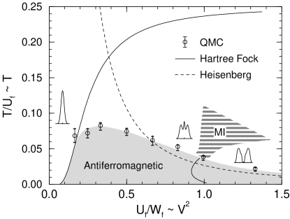
FIG. 11.: Phase diagram of the single–band Hubbard Model; 1 effective f orbital per site. The Néel temperature $T_{N}$ below which antiferromagnetic ordering takes place is indicated by the boundary between the shaded (antiferromagnetic) and unshaded regions. For small $U_{f}/W_{f}$, $T_{N}$ is well–approximated by Hartree–Fock (solid line). For large $U_{f}/W_{f}$, $T_{N}$ matches onto the spin–1/2 antiferromagnetic Heisenberg Model (dashed line). QMC, which is exact, picks up both limits and the intermediate coupling regime [80], which both Hartree Fock and Heisenberg fail to capture. The inserts show the density of states for the infinite dimensional Hubbard model, and the continuous metal-insulator (MI) transition where the central resonance is lost [83]. The solid curve below is an extension of this MI boundary which might apply were the magnetic order suppressed [83].

and “lower–Hubbard bands”, which are separated in energy by the on–site repulsion $U_{f}$. If $U_{f}$ exceeds the bandwidth of the system, this gives rise to a “Mott–Hubbard” gap at half–filling. At weak coupling, small $U_{f}/W_{f}$, these upper and lower Hubbard bands overlap, but the system remains insulating because of the doubling of the unit cell due to the antiferromagnetic order.

Considering now finite temperature, but remaining at half–filling, one finds that the Néel temperature $T_{N}$ below which antiferromagnetic ordering takes place exhibits a non–monotonic behavior with the ratio $U_{f}/W_{f}$. This is shown in Fig. 11. At weak coupling $T_{N}$ grows with $U_{f}/W_{f}$ in a manner well–described by the Stoner criterion, and manifested in the Hartree-Fock result shown by the solid curve. However, at strong coupling the single band Hubbard model maps onto the quantum spin–1/2 antiferromagnetic Heisenberg model, with exchange constant $J=4t_{f\!f}^{2}/U_{f}$. Thus at strong coupling the Hubbard model $T_{N}$ turns over and falls, as seen in the QMC results (data points) in Fig. 11 [80]. Indeed, high temperature series calculations give $T_{N}=3.83\,t_{f\!f}^{2}/U_{f}$ [81], shown by the dashed curve in Fig. 11.

It is important to realize that Hartree-Fock (HF) mean field theory completely misidentifies the strong coupling behavior of $T_{N}$, and, instead of the correct Heisenberg result, predicts that $T_{N}$ approaches $U_{f}/4$ with increasing $U_{f}/W_{f}$. At the HF Néel temperature, local moments do become well–formed, but contrary to the HF results, these moments remain unordered until much lower temperatures set by the scale $J$. The QMC calculations, on the other hand, can separately resolve these two different energy scales, either by studying the appropriate correlation functions, the local moment and the magnetic structure factor [76], or else directly from the thermodynamics [82, 78].

This single band model already includes a number of features of possible interest to the volume collapse, particularly to Johansson’s Mott transition picture [38]. QMC simulations find the evolution of the density of electrons with chemical potential shows flat plateaus indicative of a well–formed gap as the occupation per site passes through $\langle n\rangle=1$ [76]. Unlike mean-field treatments, however, the transfer of spectral weight as the ratio of $U_{f}/W_{f}$ increases is much less abrupt, and includes the development of a resonance at the Fermi surface before the formation of upper and lower Hubbard bands, as sketched in the inserts in Fig. 11 [83]. Calculations for the infinite dimensional Hubbard model suggest a continuous metal-insulator (MI) transition in the vicinity of $U_{f}/W_{f}\sim 1$ (shaded region labeled “MI”) associated with the loss of this resonance [83]. The solid line below is an artificial extension of this boundary into the antiferromagnetic region, which might apply were the magnetic order suppressed, for example, by frustrating interactions. Similar infinite dimensional calculations for the antiferromagnetic-paramagnetic boundary are in reasonable agreement with the three-dimensional QMC results in Fig. 11, suggesting the relevance of this work to the 3–d case of interest here.

The single band Hubbard model can, of course, be generalized by including longer range hopping or Coulomb interactions. Including multiple orbitals, however, allows one to describe a number of phenomena, like the screening of f–electron spins by conduction bands, which occur in rare earth systems like Ce. The most commonly considered two band Hamiltonian is the Periodic Anderson Model (PAM).

$$H = \sum_{k\sigma}\epsilon_{k}d_{k\sigma}^{\dagger}d_{k\sigma}-\sum_{k\sigma}V_{k}(d_{k\sigma}^{\dagger}f_{k\sigma}+f_{k\sigma}^{\dagger}d_{k\sigma})$$ (21)

$$+U_{f}\sum_{i}(n_{if\uparrow}-\frac{1}{2})(n_{if\downarrow}-\frac{1}{2})$$

$$+\sum_{i\sigma}\epsilon_{f}n_{if\sigma}-\mu\sum_{i\sigma}(n_{if\sigma}+n_{id\sigma})\,.$$

For the simple cubic structure considered here, we have taken

$$\epsilon_{k} = -2t_{dd}\,[\cos{k_{x}a}+\cos{k_{y}a}+\cos{k_{z}a}]\,,$$ (22)

$$V_{k} = -2t_{fd}\,[\cos{k_{x}a}+\cos{k_{y}a}+\cos{k_{z}a}]\,,$$ (23)

where $a$ is the lattice constant. We now have two sets of orbitals, $d$ and $f$. The first is “itinerant”– the valence or $d$ orbitals are hybridized on neighboring sites, giving rise to a dispersive band $\epsilon_{k}$, with no interactions, $U_{d}=0$. The second is “localized,” with a flat, non–dispersive band $\epsilon_{f}$, and also highly correlated, electrons of spin up and down repel with an on–site energy $U_{f}$. The $f$ orbitals hybridize with the itinerant $d$ band with matrix element $V_{k}$. There are different choices of $V_{k}$ used in the literature, the most common being a $k$-independent constant for which the localized and itinerant electrons hybridize on the same site. Our choice, Eq.(23), corresponds to the localized orbitals hybridizing with the near–neighbor itinerant orbitals.

The case $\epsilon_{f}\!=\!0$ is termed the “symmetric limit” of this model and, as in the single band Hubbard model, at chemical potential $\mu\!=\!0$ both the localized and itinerant orbitals are precisely half–filled for any temperature and choice of the parameters $t_{dd},t_{fd}$, and $U_{f}$ for a bipartite lattice. Again, there is no sign problem in this limit. Because of the particle-hole symmetric form in which the third term of Eq.(21) is written, this limit corresponds to the site energy choice $\varepsilon_{f}=\epsilon_{f}\!-\!U_{f}/2=-U_{f}/2$ in the notation of Fig. 6. It is our intention to eventually consider both non-symmetric limits as well as to introduce a dispersive $f$ band. Nonetheless, the present simpler case is of some interest, especially since Fig. 8 suggests the $f$–valence interaction may be the more important origin of the overall $f$-band width. From this perspective, the 1-band Hubbard Hamiltonian and the present Periodic Anderson Hamiltonian may be viewed as the simplest nontrivial correlated models within which to examine the effects of $f$–$f$ and $f$–valence interactions, respectively.

The physics of the PAM is by no means entirely sorted out. Again, it is at half–filling where our understanding is most complete. There, a competition between an “RKKY” energy scale $E_{{\rm RKKY}}\propto J^{2}/W_{d}$ and a Kondo energy scale $E_{{\rm K}}\propto W_{d}\,{\rm exp}(-W_{d}/J)$, where $J\propto t_{fd}^{2}/U_{f}$, that determines which of two possible ground states occurs. If $E_{{\rm RKKY}}$ is dominant, at low temperatures the moments on the localized orbitals organize in an antiferromagnetic pattern via a coupling mediated by the itinerant band. If $E_{{\rm K}}$ is dominant, at low temperatures the moments on the localized orbitals form singlets with electrons in the conduction band. In this phase the low temperature Curie contribution to the uniform susceptibility is suppressed, even though the localized orbitals remain singly occupied.

The phase diagram in the $T/U_{f}$–$U_{f}/W_{f}$ plane for $t_{dd}=1$ eV and $U_{f}=6$ eV is rather reminiscent of the corresponding phase diagram of the single band Hubbard Hamiltonian, where in analogy to that case we have taken $W_{f}\equiv 12\,t_{fd}$ for the PAM, as discussed at the end of Section 3. As shown in Fig. 12, there is a low temperature antiferromagnetic phase, whose transition temperature exhibits a non–monotonic dependence on $U_{f}/W_{f}$ similar to the one band case. There is also a cross–over temperature which separates the paramagnetic phase into a

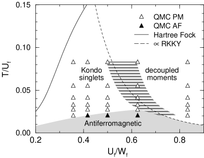
FIG. 12.: Phase diagram of the 3–d, symmetric Periodic Anderson Model (PAM) at half–filling (1 electron per orbital per site) from QMC simulations. Here $U_{f}=6t_{dd}$ is fixed, $W_{f}=12\,t_{fd}$ is varied, and the number of sites $N=4\times 4\times 4=64.$ QMC data points are shown by triangles, the dark triangles indicate antiferromagnetic ordering in the f–band. The antiferromagnetic region is indicated by shading. At higher temperatures and high $U_{f}/W_{f}$ free f–band moments still exist, but are decoupled and not ordered. As $U_{f}/W_{f}$ decreases, the f–band electrons begin to form singlets with the conduction–band electrons, until in the regime labeled “Kondo singlets” the Kondo–like singlets are fully–formed. The hashed region marks the Kondo singlet formation cross–over. Experimentally the two regimes are distinguished by the absence of a Curie–like $1/T$ divergence of the uniform susceptibility in the Kondo regime. Hartree Fock and RKKY curves are shown for comparison.

region with decoupled moments (to the right of the hatched boundary), and a region where these moments form singlets with electrons in the conduction band (to the left). This cross–over region is the counterpart of the metal-insulator transition in Fig. 11, in that in both cases this boundary is associated with appearance of the central resonance for decreasing $U_{f}/W_{f}$. The Hartree-Fock prediction for $T_{N}$ (solid curve) in Fig. 12 also has the same appearance as in Fig. 11, first rising and then saturating at $U_{f}/4$ (not shown) for increasing $U_{f}/W_{f}$. The RKKY energy, $E_{\rm RKKY}/U_{f}\propto(U_{f}/W_{f})^{-4}$ for constant $W_{d}$ and $U_{f}$, is analogous to the Heisenberg curve in Fig. 11. The ratio $E_{\rm RKKY}/U_{f}$ is plotted as the dashed curve in Fig. 12, and has been scaled to be consistent with the QMC location of $T_{N}$ near $U_{f}/W_{f}=0.6$.

The parameters in Figs. 5–8 may be used to translate the location of the observed rare earth volume collapse transitions (or symmetry changes in Nd and Sm) into values of $U_{f}/W_{f}$. Considering only the $f$-valence hopping, these are in the range $U_{f}/W_{f}=$ 1.1–1.9 except for Ce which is 3.7–2.6, as noted earlier. It is not unreasonable to associate these values with the cross–over region just discussed, $U_{f}/W_{f}\sim 0.8$ or larger if extrapolated to room temperature, whereas by contrast, the Hartree-Fock predictions for the symmetric two-band model indicate a transition for $U_{f}/W_{f}\sim 0.2$. It should also be emphasized that the one and two-band models discussed here correspond to half-filled $f$ bands, and that lower $f$-band filling should favor the “itinerant” states, pushing transitions to larger values of $U_{f}/W_{f}$, as may occur with Ce.

C Density of States in the PAM

The behavior of the quasiparticle density of states (DOS) $N(\omega/U_{f})$ provides an especially graphic illustration of how QMC differs from mean field theories such as HF in its treatment of correlations.

In Fig. 13 we show $N(\omega/U_{f})$ of the localized band of the PAM for different inverse hybridizations $U_{f}/W_{f}$ at a temperature above the Néel temperature $T_{N}$ at which antiferromagnetic ordering occurs. The DOS was obtained by numerical analytic continuation of the single–particle imaginary–time Green’s function, $G(\tau)=\frac{1}{N}\sum_{\bf p}\langle T_{\tau}c_{\bf p}(\tau)c_{\bf p}^{\dagger}(0)\rangle$, using the relation

$$G(\tau)=\int_{-\infty}^{\infty}d(\omega/U_{f}){e^{-\tau\omega/U_{f}}\over{1+e^{-\omega/T}}}N(\omega/U_{f})$$ (24)

FIG. 13.: The f-band quasi-particle density of states $N(\omega)$ as a function of distance from the Fermi energy ($\omega_{F}=0$) of the PAM for $T/U_{f}=1/30$, $U_{f}=6t_{dd}$, and at half-filling $\langle n\rangle=2$. Two values of $U_{f}/W_{f}$ are shown. For $U_{f}/W_{f}$ large, the two Hubbard-band peaks contain all of the weight in the DOS (solid line). [The solid line values have been reduced by a factor of $3$.] As $U_{f}/W_{f}$ decreases, the Kondo-singlet formation regime is entered and spectral weight shifts continually to the center, Fermi–energy region. The dot–dashed line represents a small $U_{f}/W_{f}$ where the singlets are well–formed. The pseudo–gap, or reduction in the spectral function $N(\omega)$ at the Fermi energy, is due to the insulating nature of the symmetric, half–filled PAM at small $U_{f}/W_{f}$.

for imaginary time $\tau$, temperature $T/U_{f}$, and frequency $\omega/U_{f}$. We use the maximum entropy method [84] to perform the analytic continuation in a technique which utilizes the full imaginary–time covariance matrix.

For a large $U_{f}/W_{f}$ (solid line), the spectral weight is concentrated in the lower and upper ’Hubbard’ bands, corresponding to singly–occupied localized orbitals and to doubly–occupied localized orbitals, respectively. As $U_{f}/W_{f}$ is decreased, the hybridization between the bands increases and the spectral weight simultaneously begins to shift continuously from the two peaks to the region near the Fermi energy ($\omega/U_{f}=0$). The build–up of the central peak in the DOS corresponds to the formation of singlets between electrons on the localized and itinerant orbitals as will be discussed shortly. At a sufficiently small $U_{f}/W_{f}$ a fully–developed three–peak structure is seen in the DOS (dot–dashed line). The pseudo–gap, or reduction in the spectral function $N(\omega)$ at the Fermi energy, is due to the insulating nature of the symmetric, half–filled PAM at small $U_{f}/W$.

There is no mean–field analogy either for the three peak structure in the DOS, or for this continuous shift in the spectral weight. At these same conditions, HF yields a partial $f$-DOS similar to Fig. 13 for the localized limit, $U_{f}/W_{f}=5$. However, by $U_{f}/W_{f}=0.5$, these same lower and upper Hubbard peaks are still present, although considerably broadened. Not until $U_{f}/W_{f}=0.22$, at $T/U_{f}=0.033$, do the HF antiferromagnetic and paramagnetic free energies cross, at which point a single broad central HF $f$-DOS peak is observed for smaller $U_{f}/W_{f}$.

D Magnetic Properties of the Periodic Anderson Hamiltonian

The ultimate goal of using QMC to compute precisely the contribution of the correlation energy for the volume collapse transition is still in the future, both in determining the specific appropriate lattice Hamiltonian and in then carrying out the computations. Here we will show some further results which illustrate that QMC can sensitively pick up the basic physics of correlations between moments like Kondo singlet formation and long range antiferromagnetic order. We will continue to simulate the PAM, Eq.(21) for $t_{dd}=1$ eV, $U_{f}=6$ eV, and a range of $t_{fd}$ values indicated as before by $W_{f}=12\,t_{fd}$. These results will provide some of the background to the phase diagram shown in Fig. 12.

While we are primarily interested in determining the thermodynamics to infer the equation of state, it is useful to look at magnetic properties such as the local moment and magnetic structure factor. In Fig. 14 we show the square of the local moment $\mu_{d(f)}^{2}=\langle{\bf S}_{id(f)}\cdot{\bf S}_{id(f)}\rangle$ on the itinerant ($d$) and localized ($f$) orbitals. $\mu_{d}^{2}$ takes on a

FIG. 14.: Square of the local moment on the itinerant (lower curve) and localized (upper curve) orbitals at various temperatures $T/U_{f}$ and $U_{f}/W_{f}$. The values shown have the total moment for a non-interacting system subtracted, so that $0$ on the curves corresponds to the moment of a non–interacting electron system. The itinerant orbital electrons remain at approximately the non-interacting moment value. The local (f) orbitals have increasingly well–formed moments as $U_{f}/W_{f}$ becomes larger.

value essentially equal to that for a non-interacting electron gas. This is a consequence of the lack of correlations, $U_{d}=0$, between up and down spin electrons. In contrast, $\mu_{f}^{2}$ shows a significant enhancement throughout the range of interband hybridization $t_{fd}$.

$\mu_{f}^{2}$ is the most local measure possible of magnetism– the presence or absence of a moment on a site. The magnetic structure factor determines the degree of the order between spins on different sites across the entire lattice,

$$S_{ff}(T,{\bf q}_{*}=(\pi,\pi,\pi))={1\over N}\sum_{ij}(-1)^{i+j}{\bf S}_{if}\cdot{\bf S}_{jf}\,.$$ (25)

This quantity is shown in Fig. 15 for various values of the temperature and interorbital hybridization, $t_{fd}$, reflected in the ratio $U_{f}/W_{f}$. A careful finite size scaling study is necessary before rigorous conclusions concerning the presence of long range antiferromagnetic order are drawn. The above data, however, suggest a strong tendency for the moments to order antiferromagnetically, with an ordering temperature which is maximal around $U_{f}/W_{f}\approx 0.6$.

As discussed above, singlet formation between the spins of the localized and itinerant electrons competes with antiferromagnetic order. Fig. 16 shows a quantity which measures this tendency. Here, $c_{fd}$ is essentially $\langle{\bf S}_{if}\cdot{\bf S}_{jd}\cdot\rangle$ averaged over near-neighbor pairs, $i,j$, and

FIG. 15.: Anti-ferromagnetic structure factor, $S_{ff}(T/U_{f},{\bf q}_{*}=(\pi,\pi,\pi)\,)$ for various values of $U_{f}/W_{f}$. The horizontal line demarks the existence of antiferromagnetic long–range order in the system.

appropriately normalized to reflect the number of such pairs and the average on-site local moments. The crossing of these curves through 40–60 percent of their lowest saturated value, indicated by the horizontal lines, gives an estimate of the Kondo temperature below which singlet formation takes place [85].

From the results shown in Figs. 14–16, and analysis of other quantities such as the density of states, we infer the

FIG. 16.: A measure of the tendency for Kondo singlet formation. The horizontal lines indicate the approximate range of the cross–over between the paramagnetic and Kondo singlet phases (hatched region of Fig. 12.)

magnetic phase diagram in the $(U_{f}/W_{f}$, $T/U_{f})$ plane for the PAM on a 3–d simple cubic lattice at $t_{dd}=1$ eV, $U_{f}=6$ eV, and half–filling, shown in Fig. 12.

Low–temperature HF calculations of the squared local moments, $\mu^{2}_{d(f)}$, resemble the QMC results in Fig. 14 for the antiferromagnetic phase. However, neither $f$ or $d$ moment shows any enhancement in the paramagnetic phase, demonstrating the well known fact that moment formation and magnetic order coincide in HF. Both antiferromagnetic and paramagnetic solutions exhibit values of $\langle{\bf S}_{1f}\cdot{\bf S}_{2d}\rangle$ which decrease from $\sim 0$ to $\sim-1/4$ as $U_{f}/W_{f}$ is reduced, where 1 and 2 are the two sites of a doubled unit cell. While a crude immitation of the Kondo-like behavior in Fig. 16, even at $T\!=\!0$, this variation is quite gradual, and the mean–field expectation can of course never approach the full singlet limit of $-3/4$.

E Thermodynamic Properties of the Periodic Anderson Hamiltonian

The energy can be easily measured as a function of temperature in QMC. From this data, the specific heat can be obtained, for example using a finite difference approximation for the derivative at two relatively closely spaced temperature values. A more useful way to proceed is to measure $E(T)$ on a sufficiently fine grid of temperatures and fit to a physically motivated functional form. We have chosen

$$E(T)=E(0)+\sum_{n=1}^{N}c_{n}e^{-\beta n\Delta}\,,$$ (26)

where $\Delta$ and $c_{n}$ are free parameters. $N$ is chosen to be 5–6 to compromise between allowing sufficient flexibility to pick up the full structure without overfitting. A check on this procedure is provided by computing the integrated area,

$$\int_{0}^{\infty}dT{C(T)\over T}=\sum_{n=1}^{N}{c_{n}\over n\Delta}=4\,{\rm ln}\,2-S_{0}\,.$$ (27)

Here the presence of the term $S_{0}$ is a result of the use of a finite periodic cluster where the entropy does not go to zero at $T=0$ [86]. We find this sum rule on the total entropy is obeyed to within less than 2 percent for $t_{fd}\geq 0.8$. For smaller $t_{fd}$ the system orders antiferromagnetically at temperatures below those accessed in the simulations ($T\geq 0.1$ eV), and the integral instead approaches $3\,{\rm ln}\,2-S_{0}$, correctly reflecting the missing entropy of spin ordering. Note that the QMC calculations were extended to sufficiently high temperatures to establish the large $T$ asymptotic dependence of $C(T)/T$. We have also tried other fitting forms, and find our results for the specific heat are rather insensitive to the particular functions involved.

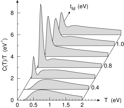
FIG. 17.: Specific heat of the PAM obtained by fitting the QMC energies. The area under the curves satisfy the sum rule, Eq. 27. The peaks in the specific heat appear to be associated with antiferromagnetic ordering. (See, also, Fig. 12.) The corresponding peaks at $t_{fd}=0.2$ and 0.4 lie below $T<0.1$ eV, the temperature range sampled by QMC, and so are absent.

The results of this procedure are shown in Fig. 17. The specific heat exhibits a broad bump at high temperatures, the energy scale $U_{f}$ of charge fluctuations, that is, excitations to the manifold of doubly occupied states. At low temperatures there is a much sharper peak which, given the data on the magnetic correlations, we believe is associated with antiferromagnetic ordering. We do not see any sharp feature associated with singlet formation, which drives the volume collapse transition according to the Kondo picture [39, 40]. However, it is well known that the signature of singlet formation in the specific heat becomes sharp only for relatively small $t_{fd}$, where, in this symmetric half–filled model, antiferromagnetism strongly competes [87].

The resolution of this difficulty is to study the PAM in parameter regimes where the antiferromagnetic order is suppressed, either by going away from the symmetric limit $\epsilon_{f}=0$ or else away from half–filling $\mu=0$. As discussed above, doing so is also suggested by the LDF analysis, where the $f$ site energy, $\varepsilon_{f}=\epsilon_{f}-U_{f}/2$, is seen in Fig. 6 to rise with compression relative to the valence chemical potential. Moreover, HF calculations show there is a significant suppression of the Néel temperature by changing $\epsilon_{f}$ or $\mu$. We have found this result using the difference in HF energies between the antiferromagnetic and ferromagnetic solutions as an estimate of $T_{N}$. This approximation gives the correct strong coupling Heisenberg scaling $T_{N}\propto t^{2}/U$ in the single band model, as opposed to $T_{N}\propto U$ which is the formally correct HF prediction obtained from looking at the temperature at which the free energy of the antiferromagnetic solution becomes lower than the paramagnetic one.

HF calculations of $C(T)/T$ for the same $4^{3}$-site two-band model bear only a gross resemblance to Fig. 17. There is the appearance of a magnetic ordering peak caused by the drop in $C(T)/T$ from antiferromagnetic to paramagnetic solutions with increasting $T$ at $T_{N}$. However, this occurs at the HF $T_{N}$ which incorrectly approaches $U_{f}/4=1.5$ eV, rather than $0$, as $t_{fd}\rightarrow 0$. Assuming the same band widths, $W_{fd}$, the rare earth transitions would occur for values of $t_{fd}$ in the range 0.1–0.3 eV for near-neighbor interactions in the simple cubic structure. At $t_{fd}=0.2$ eV, the HF paramagnetic $C(T)/T$ is in reasonable agreement with the corresponding curve in Fig. 17 except for having a larger area ($4\ln 2\!-\!2S_{0}$ versus $3\ln 2\!-\!S_{0}$). In the experimentally observed paramagnetic regime, the HF paramagnetic calculation provides a better approximation to the true thermodynamics than does the HF antiferromangnetic solution even though the latter may have lower free energy.

VI SUMMARY

This paper has discussed our current experimental and theoretical understanding of the volume collapse transitions in the trivalent rare earth metals. The data exhibit “localized” $4f$-electron behavior at low pressure, characterized by isolated-ion-like magnetic moments and the absence of these electrons in the crystal bonding, and “itinerant” $4f$-electron behavior at higher pressures, without apparent moments but with clear evidence of $4f$ bonding participation. The two regimes are separated by first order phase transitions which in three cases (Ce, Pr, and Gd) are accompanied by unusually large (9%–15%) volume changes. It is generally believed that these volume collapse transitions are associated with change in the degree of $4f$ electron correlation. Consistent with this idea, we have reported calculations of relevant parameters which indicate the transitions occur in the range $U_{f}/W_{f}=1$–2, where $U_{f}$ is the onsite Coulomb repulsion between $4f$ electrons, and $W_{f}$ is a measure of the $4f$ band width including both $f$–$f$ and $f$–valence hybridization effects. The one exception is Ce, where the transition occurs at a larger ($\sim 3$) value of this ratio which may reflect the low ($f^{1}$) $f$-band filling in this case.

We have compared a variety of orbitally realistic, mean-field based methods used to calculate these transitions: spin and orbital polarized local density functional theory, self-interaction corrections, the LDA+U method, and Hartree-Fock (HF) with static screening. As a class, these methods represent the localized phases by polarized solutions with an integer number of occupied, split-off $4f$ bands, and the itinerant phases, by a single broad collection of $4f$ bands overlapping the Fermi level. The transition is therefore accompanied by an abrupt transfer of spectral weight (the split-off bands) to the vicinity of the Fermi level. Both the loss of moment and the onset of $4f$ bonding are clear from these calculations. At very small and large volumes, $U_{f}<<W_{f}$ and $U_{f}>>W_{f}$, respectively, such mean-field solutions should provide the correct ground states, aside from mistreatment of intraatomic correlation for multi-$f$ electron atoms in the latter limit. Indeed, Anderson has used the HF solution to elucidate the limits of the one-band Hubbard model [88]. The problem lies in between these limits where competition between the two energy scales leads in general to a correlated solution. Thus, while several calculations have reported reasonable agreement with experiment for the location of the transitions [57]–[61], there are substantial differences between HF and exact Quantum Monte Carlo (QMC) solutions for few band Hamiltonians which raise doubts about these approaches.

To assess correlation effects, we have reviewed exact QMC solutions for the one band Hubbard model, and reported new QMC results for the two-band periodic Anderson lattice model. We contrast both solutions with HF results for the same Hamitonians. The QMC results for both one and two-band models show non-monotonic behavior of the Néel temperature, $T_{N}$, as a function of $U_{f}/W_{f}$, where this ratio scales like volume to a power $\sim 2$. $T_{N}$ first rises with increasing $U_{f}/W_{f}$ as antiferromagnetic order accompanies moment formation, and then falls as decreasing exchange interactions lead to moment disorder. HF misses the latter effect, so that its $T_{N}$ continues to rise to a large saturation value of $U_{f}/4\sim 1.5$ eV. The HF transitions are therefore always intrinsically associated with both moment formation and magnetic ordering. The region of magnetic order is greatly suppressed in the QMC solutions, e.g., lying below $\sim 0.1$ eV for the present PAM results based on realistic parameters. This value can be further suppressed by changing the $f$ level position (non-symmetric PAM), consistent with the experimental observation that the volume collapse transitions occur entirely within the paramagnetic regime.

The dramatic new feature in the correlated QMC solutions, which has no counterpart in mean field, is the three peak structure in the $f$ density of states (DOS) found especially at temperatures just above the region of magnetic order. The growth of the central Fermi-level resonance for decreasing $U_{f}/W_{f}$ comes from a continuous transfer of spectral weight from the outer split peaks, and is accompanied in the QMC results with reduction of the magnetic moment as might be deduced from the magnetic susceptibility. This reduction occurs at considerably larger values of $U_{f}/W_{f}$ or volume than does the HF transition, and is in much better agreement with our “experimental” $U_{f}/W_{f}$ placement of the collapse transitions.

The central resonance is the well known signature of the Kondo effect for the PAM, and in its impurity Anderson model context, the critical aspect of the Kondo volume collapse model for Ce [39, 40]. However, it is intriguing that the infinite dimensional one-band Hubbard model reduces formally to the impurity Anderson model and exhibits a similar central resonance, which might be associated with $f$ electrons screening their own moments [83]. This blurs the distinction between the Mott transition picture [38], traditionally associated with the Hubbard model, and the Kondo volume collapse [39, 40]. The distinction is further complicated in any mean field approach which would pick up only half (e.g., $f_{\uparrow}d_{\downarrow}$ but not $f_{\downarrow}d_{\uparrow}$) of a Kondo like singlet, and might therefore still look like $f$ magnetic order. This is not the case for QMC calculations which can separately identify reduction in the local moments as well as their screening by the valence electrons, as seen in the present PAM results. More definitive use of QMC in this manner, however, awaits studies in other parameter regimes (e.g., non symmetric PAM) in search of thermodynamic features, for example, which might unambiguously demonstrate that the given model does indeed capture the essential nature of the rare earth volume collapse transitions.

A natural future direction for the theory of the rare earth volume collapse transitions would be to compromise between the all-orbital mean-field based methods and few-orbital exact treatments, so as to incorporate only the most important correlation effects within a sufficiently rich multi-orbital framework. There appears to be, for example, a growing awareness that some form of dynamic screening is critical to incorporate features such as the three peak density of states, requiring inclusion of an energy-dependent self-energy. Some success has been achieved with local, k-independent approximations to such self energies [89, 90, 91]. In principal this approach reduces to a correlated impurity problem which could be solved by QMC methods for far more orbitals per site that possible in the fully correlated lattice. Should intermediate or longer-range correlations be critical, a new modified dynamical mean field technique may allow inclusion of such correlations in addition to multiple bands [92]. All of these techniques form a bridge between local density functional methods which serve to define realistic multi-orbital Hamiltonians which may then be solved by correlated approaches such as QMC.

Prepared for a 1998 issue of the Journal of Computer-Aided Materials Design

REFERENCES

- [1] Benedict, U., J. Alloys Comp. 193 (1993) 88.
- [2] Holzapfel, W.B., J. Alloys Comp. 223 (1995) 170.
- [3] Brooks, M.S.S., Johansson, B. and Skriver, H.L., in Freeman, A.J. and Lander, G.H. (Eds) Handbook on the Physics and Chemistry of the Actinides, Vol. 1, North-Holland, Amsterdam, 1984, p. 153.
- [4] See, e.g., articles in Gschneidner, Jr. K.A. and Eyring, L.R. (Eds), Handbook on the Physics and Chemistry of Rare Earths, North-Holland, Amsterdam, 1978, Vol. 1: Metals.
- [5] See., e.g., articles in Freeman, A.J. and Lander, G.H. (Eds), Handbook on the Physics and Chemistry of the Actinides, North-Holland, Amsterdam, 1984, Vols. 1–3.
- [6] Söderlind, P., Adv. Phys., in press.
- [7] Olsen, J.S., Gerward, L., Benedict, U., Itié, J.P., Physica 133B (1985) 129.
- [8] Mao, H.K., Hazen, R.M., Bell, P.M., Wittig, J., J. Appl. Phys. 52 (1981) 4572.
- [9] Smith, G.S. and Akella, J., J. Appl. Phys. 53 (1982) 9212.
- [10] Grosshans, W.A. and Holzapfel, W.B., J. Phys. (Paris) 45 (1984) C8.
- [11] Zhao, Y.C., Porsch, F., and Holzapfel, W.B., Phys. Rev. B 52 (1995) 134. This paper suggests a 13% volume change for the room temperature volume collapse in Pr.
- [12] Akella, J., Xu, J., Smith, G.S., Physica 139 & 140 B (1986) 285; Akella, J. and Smith, G.S., J. Less-Common Met. 116 (1986) 313.
- [13] Grosshans, W.A., Ph.D. thesis, University of Paderborn, 1987.
- [14] Haire, R.G., Heathman, S., and Benedict, U., High Pres. Res. 2 (1990) 273.
- [15] Olsen, J.S., Steenstrup, S., Gerward, L., Benedict, U., Akella, J., and Smith. G., High Press. Res. 4 (1990) 366. Following [17], the last four points of this work are not included in Fig. 1.
- [16] Vohra, Y.K., Akella, J., Weir, S., and Smith, G.S., Phys. Lett. A 158 (1991) 89.
- [17] Zhao, Y.C., Porsch, F., and Holzapfel, W.B., Phys. Rev. B 50 (1994) 6603.
- [18] Akella, J., Smith, G.S., and Jephcoat, A.P., J. Phys. Chem. Solids. 49 (1988) 573.
- [19] Akella, J., Weir S.T., Hua, H., Vohra, Y.K., Rev. High Pres. Sci. & Tech. 7 (1998), in press. The volumes from the author’s two “modified universal equation of state” fits give a collapse of 10.6% at 59 GPa relative to the large volume side of the transition.
- [20] Grosshans, W.A., Vohra, Y.K., and Holzapfel, W.B., Phys. Rev. Lett. 49 (1982) 1572.
- [21] Smith, G.S., and Akella, J., Phys. Lett. 105A, (1984) 132.
- [22] Vohra, Y.K., Vijayakumar, V., Godwal, B.K., and Sikka, S.K., Phys. Rev. B 30 (1984) 6205.
- [23] Hamaya, N., Sakamoto, Y., Fujihisa, H., Fujii, Y., Takemura, K., Kikegawa, T., and Shimomura, O., J. Phys.: Condens. Matter 5 (1993) L369.
- [24] Porsch, F., Holzapfel, W.B., Phys. Rev. B 50 (1994) 16212.
- [25] Seipel, M., Porsch, F., and Holzapfel, W.B., High Pres. Res. 15 (1997) 321.
- [26] Johansson, B., and Rosengren, A., Phys. Rev. B 11, 2836 (1975).
- [27] Vohra, Y.K., Olijnik, H., Grosshans, W., and Holzapfel, W.B., Phys. Rev. Lett. 47 (1981) 1065.
- [28] Duthie, J.C. and Pettifor, D.G., Phys. Rev. Lett. 38 (1977) 564.
- [29] Skriver, H.L., in Sinha, S.P. (Ed.) Systematics and the Properties of the Lanthanides, Reidel Publishing Co., Dordrecht, 1983, p. 213.
- [30] Skriver, H.L. Phys. Rev. B 31 (1985) 1909.
- [31] See., e.g., discussion and references in Ravindran, P., Nordström, L., Ahuja, R., Wills, J.M., Johansson, B., and Eriksson, O., Phys. Rev. B 57 (1998) 2091.
- [32] Söderlind,P., Eriksson, O., Johansson, B., Wills, J.M., and Boring, A.M., Nature 374 (1995) 524.
- [33] Söderlind, P., Eriksson, O., Johansson, B., Wills, J.M., Phys. Rev. B 52 (1995) 13169.
- [34] Vohra, Y.K., and Akella, J., Phys. Rev. Lett. 67 (1991) 3563; ibid, High Press. Res. 10 (1992) 681.
- [35] Akella, J., Weir, S., Wills, J.M., Söderlind, P., J. Phys.: Condens. Mat. 9 (1997) L549.
- [36] Johansson, B., Phys. Rev. B 15 (1977) 5890.
- [37] Young, D.A., Phase Diagrams of the Elements, University of California Press, Berkeley, 1991.
- [38] Johansson, B., Philos. Mag. 30 (1974) 30.
- [39] Allen, J.W. and Martin, R.M., Phys. Rev. Lett. 49 (1982) 1106; Allen, J.W. and Liu, L.Z. Phys. Rev. 46 (1992) 5047.
- [40] Lavagna, M., Lacroix, C. and Cyrot, M., Phys. Lett. 90A (1982) 210; J. Phys. F 13 (1983), 1008.
- [41] McEwen, K.A., in Gschneidner, Jr., K.A. and Eyring L.R. (Eds) Handbook on the Physics and Chemistry of Rare Earths, North-Holland, Amsterdam, 1978, Vol. 1 – metals, p. 411, see Table 6.1.
- [42] Ward, J.W., Kleinschmidt, P.D. and Peterson, D.E., in Freeman, A.J. and Keller, C., (Eds), Handbook on the Physics and Chemistry of the Actinides, North-Holland, Amsterdam, 1986, Vol. 4, p. 309.
- [43] Mller, H.B., Jensen, J.Z., Wulff, M., Mackintosh, A.R., McMasters, O.D. and Gschneidner, Jr., K.A., Phys. Rev. Lett. 49 (1982) 482.
- [44] McMahan, A.K., in Kaplan, T.A. and Mahanti, S.D., Electronic Properties of Solids Using Cluster Methods, Plenum Press, New York, 1995, p. 157.
- [45] Andersen, O.K., Phys. Rev. B 12 (1975) 3060.
- [46] Skriver, H.L., The LMTO Method, Springer, Berlin, 1984.
- [47] McMahan, A.K., Martin, R.M., Satpathy, S., Phys. Rev. 38 (1988) 6650.
- [48] McMahan, A.K., Annett, J.F., and Martin, R.M., Phys. Rev. B 42 (1990) 6268.
- [49] Herbst, J.F. and Wilkins, J.W., in Gschneidner, Jr., K.A., Eyring, L, and Hüfner, S. (Eds), Handbook on the Physics and Chemistry of Rare Earths, Vol. 10, p. 321.
- [50] Boring, A.M., Albers, R.C., Eriksson, O., and Koelling, D.D., Phys. Rev. Lett. 68 (1992) 2652.
- [51] Hohenberg, P. and Kohn, W., Phys. Rev. 136 (1964) B864.
- [52] Jones, R.O. and Gunnarsson, O., Rev. Mod. Phys. 61 (1989) 689.
- [53] Skriver, H.L., Andersen, O.K. and Johansson, B., Phys. Rev. Lett. 41 (1978) 42.
- [54] Skriver, H.L., Andersen, O.K. and Johansson, B., Phys. Rev. Lett. 44 (1980) 1230.
- [55] Glötzel, D., J. Phys. F. 8 (1978) L163. Phys. Rev. Lett. 44 (1980) 1230.
- [56] Skriver, H.L. in Schilling, J.S. and Shelton, R.N. (Eds), Physics of Solids Under High Pressure, North-Holland, Amsterdam, 1981, p. 279.
- [57] Eriksson, O., Brooks, M.S.S. and Johansson, B., Phys. Rev. B 41 (1990) 7311.
- [58] Svane, A., Trygg, J., Johansson, B., and Eriksson, O., Phys. Rev. B 56 (1997) 7143.
- [59] Szotek, Z., Temmerman, W.M., and Winter, H., Phys. Rev. Lett. 72 (1994) 1244
- [60] Svane, A., Phys. Rev. Lett., 72 (1994), 1248.
- [61] Svane, A., Phys. Rev. B 53 (1996) 4275.
- [62] Sandalov, I.S., Hjortstam, O., Johansson, B. and Eriksson, O., Phys. Rev. B. 51 (1995) 13987.
- [63] Mazin, I.I. and Anisimov, V.I., Phys. Rev. B 55 (1997) 12822.
- [64] Anisimov,V.I., Zaanen, J. and Andersen, O.K., Phys. Rev. B 44 (1991) 943; Anisimov, V.I., Aryasetiawan, F., and Lichtenstein, A.I., J. Phys. Condens. Matter 9 (1997) 767.
- [65] Temmerman, W.M., Szotek, Z. and Winter, H., Phys. Rev. B 47 (1993) 1184.
- [66] Bulut, N., Scalapino, D.J., and White, S.R., Phys. Rev. B 50 (1994) 9623.
- [67] Mann, J.B., Atomic Structure Calculations, Los Alamos Sci. Lab. Report LA-3690, May 1967.
- [68] The bare for Ni is eV [67], and is evident in the gap between occupied and empty Ni states in recent Hartree-Fock calculations for NiO: Towler, M.D., Allan, N.L., Harrison, N.M., Saunder, V.R., Mackrodt, W.C., Aprà, E., Phys. Rev. B 50 (1994) 5041.
- [69] Surh,M.P., private communication. See also references and discussion in the second paper in [64], which compares the LDA+U method to the GW approximation.
- [70] Scalettar, R.T., White, S.R., Scalapino, D.J., and Sugar, R.L., Phys. Rev. B44, (1991) 770.
- [71] Lundin, U., Eriksson, O., Johansson, B., and Sandalov, I., Physica 230-232 (1997) 445.
- [72] Dagotto, E., Reviews of Modern Physics, 66, (1994) 763.
- [73] Vekic, M., Cannon, J.W., Scalapino, D.J., Scalettar, R.T., and Sugar, R.L., Phys. Rev. Lett. 74, (1995) 2367.
- [74] Motome, Y., and Imada, M., Journal of the Physical Society of Japan, 66, (1997) 1872.
- [75] Huse, D.A., Phys. Rev. B 37 (1988) 2380.
- [76] White, S.R., Scalapino, D.J., Sugar, R.L., Loh, Jr., E.Y., Gubernatis, J.E., and Scalettar, R.T., Phys. Rev. B 40 (1989) 506.
- [77] Blankenbecler, R., Scalapino, D.J., and R.L. Sugar, R.L., Phys. Rev. 24 (1981) 2278.
- [78] Duffy, D. and Moreo, A., Phys. Rev. B 55 (1997) 12918.
- [79] Montorsi, A., Ed., The Hubbard Model, World Scientific, 1992.
- [80] Scalettar, R.T., Scalapino, D.J., Sugar, R.L., and Toussaint, D., Phys. Rev. B 39 (1989) 4711.
- [81] Rushbrook, G.S., Baker Jr., G.A., and Wood, P.J., in Comb, C. and Green, M.S. (Eds) Phase Transitions and Critical Phenomena, Vol. 3, Academic, New York, p. 245.
- [82] Scalettar, R.T., Scalapino, D.J., Sugar, R.L., and Toussaint, D., Phys. Rev. B 36 (1987) 8632.
- [83] Jarrell, M. and Pruschke, T., Z. Phys. B 90 (1993) 187; Pruschke, T., Cox., D.L. and Jarrell, M.,Phys. Rev. B 47 (1993) 3553.
- [84] Jarrell, M., and Gubernatis, J.E., Phys. Rep. 269 (1996) 135.
- [85] For the single-impurity Anderson Model, one may obtain from fitting the spin susceptibility to a low-temperature solution. Hirsch, J.E., and Fye, R.M., Phys. Rev. Lett. 56, 2521 (1986). Here, we note that both the interband moment and and the spin susceptibility saturate as singlets are formed, and use the saturation of the interband moment as the signal of singlet formation.
- [86] The value of is determined by the one–body part of the Hamiltonian. It has been separately calculated and agrees with the QMC results. for Eq.(22) and sites.
- [87] A peak is seen in the specific heat when . Hewson, A.C., The Kondo Problem to Heavy Fermions, 157 (Cambridge 1993) [s-d model].
- [88] Anderson, P.W., Concepts in Solids, W. A. Benjamin, Inc., Reading, 1963, p. 157.
- [89] Steiner, M.M., Albers, R.C. and Sham, L.J., Phys. Rev. B 45 (1992) 13272.
- [90] Han, J.E., Alouani, M. and Cox, D.L., Phys. Rev. Lett. 78 (1997) 939.
- [91] Lichtenstein, A.I. and Katsnelson, M.I., Phys. Rev. B 57 (1998) 6884.
- [92] Hettler, M.H., Tahvildar-Zadeh, A.N., Jarrell, M., Prushke, T., and Krishnamurthy, H.R., unpublished (cond-mat/9803295).