Kondo Effect in Single Quantum Dot Systems
— Study with Numerical Renormalization Group Method —

1 Introduction

Coulomb oscillations behavior in quantum dot systems is well known as one of the typical phenomena due to the Coulomb repulsion between electrons in the dot. But it is one aspect of the electron-electron interaction effects. Local spin moment is induced by the Coulomb repulsion in the dot sometime. It will fluctuate by exchanging spin moment with leads and thus cause the strong inelastic scattering. But the local spin disappears in the lowest temperature due to the spin singlet formation between leads and the dot. These effects have been investigated as the Kondo effect for the magnetic impurity systems in many years, ${}^{\hbox{\immediate{\bf{?}})}}$ and for the quantum dot systems recently. ${}^{\hbox{\immediate{\bf{?}},\penalty 1000\hskip 0.91003pt plus 0.70004pt minus 0.70004pt{\bf{?}},\penalty 1000\hskip 0.91003pt plus 0.70004pt minus 0.70004pt{\bf{?}},\penalty 1000\hskip 0.91003pt plus 0.70004pt minus 0.70004pt{\bf{?}},\penalty 1000\hskip 0.91003pt plus 0.70004pt minus 0.70004pt{\bf{?}},\penalty 1000\hskip 0.91003pt plus 0.70004pt minus 0.70004pt{\bf{?}},\penalty 1000\hskip 0.91003pt plus 0.70004pt minus 0.70004pt{\bf{?}},\penalty 1000\hskip 0.91003pt plus 0.70004pt minus 0.70004pt{\bf{?}},\penalty 1000\hskip 0.91003pt plus 0.70004pt minus 0.70004pt{\bf{?}},\penalty 1000\hskip 0.91003pt plus 0.70004pt minus 0.70004pt{\bf{?}})}}$

The origins of the non-vanishing spin moment in the dot are not unique. Of course unpaired electron in the odd number electrons in the dot brings the spin moment. Furthermore, degenerate orbitals, or strong Hund’s rule coupling can induce the non-vanishing spin moment even in the even electron number cases. ${}^{\hbox{\immediate{\bf{?}})}}$ This will cause varieties in the behavior of the spin state when the electron number is changed by the gate voltage. In the low temperature range that the Kondo singlet state is formed, the inelastic scattering due to the spin fluctuation is suppressed. Therefore the coherent process will dominate the tunneling. This process is considered as the resonant tunneling through the Kondo peak at the Fermi level in some sense. The Kondo peak sensitively diminishes as the temperature increases and disappears at high temperatures because the characteristic temperature for the many body singlet formation, the Kondo temperature, is usually very low. In general, the tunneling conductance will show various types of the interference effect depending on the geometry and the connectivity of the dot systems. The coherency of the system is disturbed by the inelastic scattering due to the spin moment revived at finite temperatures. However, calculation of the conductance in such the intermediate temperature has not been done theoretically because the reliable method to treat the Kondo effect has not been established.

In this paper, we consider the system shown in Fig. 1, a quantum dot and connected two leads.

Fig.  1: The configuration of the system. The $z$-axis is perpendicular to the $xy$ plane.

We calculate the tunneling conductance in wide temperature range from the high temperature region in which the usual Coulomb oscillations are observed, to the lower temperature region in which the Kondo singlet state is formed. Conductance is calculated as the function of the gate voltage. We assume that two orbitals of the dot are active for the tunneling process. The following two cases are considered for the tunneling Hamiltonian (TH) between the conduction channels in the leads and the orbitals in the dot: (THi) There is one conduction channel in each lead, and it hybridizes with both of two orbitals in the dot. This means that the tunneling processes via the two orbitals interfere each other. (THii) There are two conduction channels in each lead, and each of the channels hybridizes separately with one of two orbitals in the dot. In this case the tunneling processes of the two channels are independent and do not interfere. (But the electronic state of the dot itself is affected by the interaction between electrons in the different channels.) In such two situations, we study the following three cases for the orbital state in the dot; (1) orbital energies in the dot are not degenerate, (2) orbital energies in the dot are degenerate, (3) electrons on the orbitals have strong Hund’s rule coupling. The six combinations of the situation, from THi-1 to THii-3, are studied systematically.

There have been several methods to calculate the conductance in finite temperatures; perturbation theory, non-crossing approximation, quantum Monte Calro method, numerical renormalization group (NRG) method. ${}^{\hbox{\immediate{?},\penalty 1000\hskip 0.91003pt plus 0.70004pt minus 0.70004pt{?},\penalty 1000\hskip 0.91003pt plus 0.70004pt minus 0.70004pt{?},\penalty 1000\hskip 0.91003pt plus 0.70004pt minus 0.70004pt{?},\penalty 1000\hskip 0.91003pt plus 0.70004pt minus 0.70004pt{?},\penalty 1000\hskip 0.91003pt plus 0.70004pt minus 0.70004pt{?})}}$ The NRG is a reliable method in the temperature region $T\mathrel{\mathchoice{\lower 2.58334pt\vbox{\halign{$\m@th\displaystyle\hfil#\hfil$\cr<\crcr\sim\crcr}}}{\lower 2.58334pt\vbox{\halign{$\m@th\textstyle\hfil#\hfil$\cr<\crcr\sim\crcr}}}{\lower 2.58334pt\vbox{\halign{$\m@th\scriptstyle\hfil#\hfil$\cr<\crcr\sim\crcr}}}{\lower 2.58334pt\vbox{\halign{$\m@th\scriptscriptstyle\hfil#\hfil$\cr<\crcr\sim\crcr}}}}T_{\rm K}$, where $T_{\rm K}$ is the Kondo temperature. ${}^{\hbox{\immediate{?},\penalty 1000\hskip 0.91003pt plus 0.70004pt minus 0.70004pt{\bf{?}},\penalty 1000\hskip 0.91003pt plus 0.70004pt minus 0.70004pt{\bf{?}},\penalty 1000\hskip 0.91003pt plus 0.70004pt minus 0.70004pt{\bf{?}})}}$ This method directly calculates the tunneling matrices between wave functions of many electron states. Therefore we can obtain the tunneling probabilities in a general way for the coherent process in the low temperatures and the incoherent process in the high temperatures. The numerical calculations are performed by using NRG method through this paper.

We found that the tunneling through the Kondo resonance fully develops in the temperature region, $T\mathrel{\mathchoice{\lower 2.58334pt\vbox{\halign{$\m@th\displaystyle\hfil#\hfil$\cr<\crcr\sim\crcr}}}{\lower 2.58334pt\vbox{\halign{$\m@th\textstyle\hfil#\hfil$\cr<\crcr\sim\crcr}}}{\lower 2.58334pt\vbox{\halign{$\m@th\scriptstyle\hfil#\hfil$\cr<\crcr\sim\crcr}}}{\lower 2.58334pt\vbox{\halign{$\m@th\scriptscriptstyle\hfil#\hfil$\cr<\crcr\sim\crcr}}}}0.1T_{\rm K}^{*}\sim 0.2T_{\rm K}^{*}$, where $T_{\rm K}^{*}$ is the lowest Kondo temperature of the dot system when the gate voltage is varied. The interference effect of the tunneling process also becomes important in this region. In high temperature region $T\gg T_{\rm K}^{*}$, the Coulomb oscillations type conductance is observed commonly. In the intermediate temperature range among these, various types of conductance behaviors appear, especially in THi cases, because the coherency of each orbital channel is sensitively changed by the temperature and the gate voltage.

In §2, the cases classified to the THi are studied, and the cases classified to the THii are studied in §3. In §4, summary and discussion of this study are given.

2 One Conduction Channel in Each Lead

To study the system shown in Fig. 1, following things are contained in the model: i) Electronic states in the two leads are written as the conduction band states. ii) There are two orbitals in the dot. iii) Electron-electron interactions in the dot are considered. And, iv) the electrons have tunneling matrices between the leads and the dot. For simplicity, we consider the situation that there are only two orbitals in the dot instead of considering many orbitals. We assume that the system has the mirror symmetry with respect to the $yz$ and $zx$ planes. (The $z$-axis is perpendicular to the $xy$ plane.)

In this section, we discuss the situation classified to the THi that there are only one conduction channel in each lead, and tunneling processes via the different orbital channels interfere each other. We consider the one-dimensional degree of freedom in each lead. This situation would appear in the case that leads are very narrow, or the joint part between the leads and the dot are very narrow.

2.1 Model Hamiltonian

We consider the two orbitals in the dot, which are even and odd, respectively, under the $yz$ mirror, and are even under the $zx$ mirror. These orbitals in the dot are named as the even orbital and the odd orbital, respectively. We consider the one-dimensional degree of freedom with even symmetry under the $zx$ mirror in each lead. We use the following Anderson Hamiltonian,

$$H = H_{\rm l}+H_{\rm d}+H_{\rm l-d},$$ (2.1)

$$H_{\rm l} = \sum_{k\sigma}\varepsilon_{k}c_{{\rm L}k\sigma}^{\dagger}c_{{\rm L}k\sigma}+\sum_{k\sigma}\varepsilon_{k}c_{{\rm R}k\sigma}^{\dagger}c_{{\rm R}k\sigma},$$ (2.2)

$$H_{\rm d} = (\varepsilon_{\rm d}-t)\sum_{\sigma}n_{{\rm e}\sigma}+(\varepsilon_{\rm d}+t)\sum_{\sigma}n_{{\rm o}\sigma}$$ (2.3)

$$+U\sum_{p={\rm e,o}}n_{p\uparrow}n_{p\downarrow}+U\sum_{\sigma,\sigma^{{}^{\prime}}}n_{{\rm e}\sigma}n_{{\rm o}\sigma^{{}^{\prime}}}$$

$$+J_{\rm H}\sum_{\sigma_{1}\sigma_{2}\sigma_{3}\sigma_{4}}({\mbox{\boldmath$\sigma$}})_{\sigma_{1}\sigma_{2}}\cdot({\mbox{\boldmath$\sigma$}})_{\sigma_{3}\sigma_{4}}d_{{\rm e}\sigma_{1}}^{\dagger}d_{{\rm e}\sigma_{2}}d_{{\rm o}\sigma_{3}}^{\dagger}d_{{\rm o}\sigma_{4}},$$

$$H_{\rm l-d} = \frac{1}{\sqrt{2}}\sum_{k\sigma}V_{\rm e}d_{{\rm e}\sigma}^{\dagger}\left(c_{{\rm L}k\sigma}+c_{{\rm R}k\sigma}\right)+\frac{1}{\sqrt{2}}\sum_{k\sigma}V_{\rm o}d_{{\rm o}\sigma}^{\dagger}\left(c_{{\rm L}k\sigma}-c_{{\rm R}k\sigma}\right)+{\rm h.c.}$$ (2.4)

The terms $H_{\rm l}$ and $H_{\rm d}$ give the electron orbitals in the two leads and in the dot, respectively. The term $H_{{\rm l-d}}$ gives the electron tunneling between the two leads and the dot. The annihilation operator of the left (right) lead state is denoted by $c_{{\rm L}k\sigma}$ ($c_{{\rm R}k\sigma}$), and that of the even (odd) orbital in the dot is denoted by $d_{{\rm e}\sigma}$ ($d_{{\rm o}\sigma}$). The quantity $\varepsilon_{k}$ is the energy of the lead state. The quantity $\varepsilon_{\rm d}$ corresponds to dot’s potential, and is able to change by applying gate voltage. The energy level of the even (odd) orbital is given by $\varepsilon_{\rm d}-t$ ($\varepsilon_{\rm d}+t$). The energy separation between the even and odd orbitals is defined as $\Delta\varepsilon_{\rm d}\equiv 2t$. The Coulomb interaction constant is given by $U$ for both the intra- and inter-orbital terms. We consider the exchange interaction between electrons on the even and odd orbitals with strength $J_{\rm H}$. The operator $\sigma$ is the Pauli matrix. The quantity $V_{\rm e}$ ($V_{\rm o}$) is the hybridization matrix for the even (odd) orbital. (We neglect the $k$ dependence of the tunneling matrices.)

We introduce the even and the odd combinations of the lead orbitals, $s_{k\sigma}=(c_{{\rm L}k\sigma}+c_{{\rm R}k\sigma})/\sqrt{2}$ and $a_{k\sigma}=(c_{{\rm L}k\sigma}-c_{{\rm R}k\sigma})/\sqrt{2}$, respectively. The terms $H_{\rm l}$ and $H_{\rm l-d}$ are rewritten as,

$$H_{{\rm l}} = \sum_{k\sigma}\varepsilon_{k}s_{k\sigma}^{\dagger}s_{k\sigma}+\sum_{k\sigma}\varepsilon_{k}a_{k\sigma}^{\dagger}a_{k\sigma},$$ (2.5)

$$H_{{\rm l-d}} = \sum_{k\sigma}\left(V_{\rm e}d_{{\rm e}\sigma}^{\dagger}s_{k\sigma}+{\rm h.c.}\right)+\sum_{k\sigma}\left(V_{\rm o}d_{{\rm o}\sigma}^{\dagger}a_{k\sigma}+{\rm h.c.}\right).$$ (2.6)

The hybridization strength for the even (odd) orbital channel is denoted as $\Delta_{\rm e}=\pi V_{\rm e}^{2}\rho(\varepsilon_{\rm F})$ ($\Delta_{\rm o}=\pi V_{\rm o}^{2}\rho(\varepsilon_{\rm F})$), where $\rho(\varepsilon_{\rm F})$ is the density of states of the lead states. Hereafter we denote the even and the odd orbitals by $p$ as $p={\rm e}$ and $p={\rm o}$, respectively.

2.2 Linear response conductance

In this paper we restrict ourselves to the linear response conductance for the applied bias voltage between the left and the right leads. We generally define an electric current from the left lead L to the right lead R as follows;

$$I \equiv -e\frac{-\langle\dot{N_{\rm L}}\rangle+\langle\dot{N_{\rm R}}\rangle}{2},$$ (2.7)

where $-e$ is the charge of an electron, $\langle\dot{N_{\rm L}}\rangle$ is the expectation value of the time differentiation of the electron number operator in the lead L. The quantity $\langle\dot{N_{\rm R}}\rangle$ is that of the lead R. We obtain the following expression for the linear response conductance formula, ${}^{\hbox{\immediate{\bf{?}})}}$

$$G \equiv \frac{I}{2V}$$ (2.8)

$$= \frac{2e^{2}}{h}\lim_{\omega\rightarrow 0}\frac{P^{{}^{\prime\prime}}(\omega)}{\omega},$$

with

$$P^{{}^{\prime\prime}}(\omega) = \frac{\pi^{2}\hbar^{2}}{4}\frac{1}{Z}\sum_{n,m}\left({\rm e}^{-\beta E_{m}}-{\rm e}^{-\beta E_{n}}\right)$$ (2.9)

$$\times\left|\langle n\left|\dot{N_{\rm L}}-\dot{N_{\rm R}}\right|m\rangle\right|^{2}$$

$$\times\delta\left(\omega-\left(E_{n}-E_{m}\right)\right),$$

where $Z=\sum_{n}e^{-\beta E_{n}}$ is the partition function, $\beta$ is the inverse of the temperature, $\beta=1/T$. (See Appendix of the ref. ? for the derivation of eqs. (2.8) and (2.9).) We note that we do not have done restrictive assumptions for the electric current such as the ‘coherent tunneling’ or the ‘sequential tunneling’ in the derivation of (2.8). The conductance for the case of THi, $G^{(1)}$, is calculated by using eqs. (2.8) and (2.9) with $N_{\rm L}=\sum_{k\sigma}c_{{\rm L}k\sigma}^{\dagger}c_{{\rm L}k\sigma}$ and $N_{\rm R}=\sum_{k\sigma}c_{{\rm R}k\sigma}^{\dagger}c_{{\rm R}k\sigma}$. We note that the tunneling processes via the even and the odd orbitals interfere each other in the tunneling between leads. Following the method described in ref. ?, the current spectrum, $P^{{}^{\prime\prime}}(\omega)$, is calculated by NRG method.

Here we briefly consider the tunneling at absolute zero temperature. The system would be the local Fermi liquid state at very low temperatures. In this case there are no spin scattering processes. In such the coherent tunneling process at zero temperature, the conductance for the case of THi, $G_{\rm F}^{(1)}$, is written as follows; ${}^{\hbox{\immediate{?},\penalty 1000\hskip 0.91003pt plus 0.70004pt minus 0.70004pt{?})}}$

$$G_{\rm F}^{(1)} = \frac{2e^{2}}{h}\sin^{2}\left\{\frac{\pi}{2}\left(\langle n_{\rm e}\rangle-\langle n_{\rm o}\rangle\right)\right\}.$$ (2.10)

This expression is the extension of the relation $G_{\rm F}=(2e^{2}/h)\sin^{2}\left\{\left(\pi/2\right)\langle n\rangle\right\}$ for the single orbital case. ${}^{\hbox{\immediate{?},\penalty 1000\hskip 0.91003pt plus 0.70004pt minus 0.70004pt{?})}}$ The quantity $\langle n_{\rm e}\rangle-\langle n_{\rm o}\rangle$ appears through the interference of the tunneling processes via the even and odd orbitals. In derivation of eq. (2.10), we have applied Friedel’s sum rule to the even and the odd orbital channels separately. ${}^{\hbox{\immediate{\bf{?}},\penalty 1000\hskip 0.91003pt plus 0.70004pt minus 0.70004pt{\bf{?}},\penalty 1000\hskip 0.91003pt plus 0.70004pt minus 0.70004pt{\bf{?}})}}$

2.3 Numerical results with NRG method

2.3.1 Non-degenerate orbital case

In this subsection we present the numerical results for the non-degenerate orbital case. The parameters are chosen to satisfy the relations $\Delta_{\rm e},\Delta_{\rm o}\ll\Delta\varepsilon_{\rm d}$: $\Delta_{\rm e}=0.003\pi$, $\Delta_{\rm o}=0.002\pi$, $\Delta\varepsilon_{\rm d}=0.1$, $U=0.1$ and $J_{\rm H}=0$. (In this paper we choose the band width $D$ as an energy unit. The density of states for the conduction bands in each orbital channel are assumed to be constant within the region $-1<\omega/D<1$.)

First we present the electron occupation numbers at absolute zero temperature, $\langle n_{p}\rangle$, as a function of the dot’s potential, $\varepsilon_{\rm d}$. The conductance $G_{\rm F}^{(1)}$ at $T=0$, which is calculated from (2.10), is also shown in Fig. 2. (The conductance $G_{\rm F}^{(2)}$ at $T=0$ for the case of THii is also shown in the same figure. This quantity will be discussed in §3.)

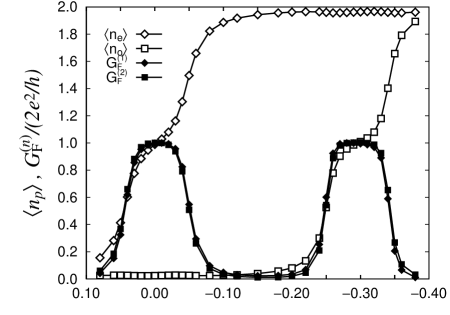
Fig.  2: The expectation value of the electron occupation numbers $\langle n_{p}\rangle$ for the even ($p={\rm e}$) and the odd ($p={\rm o}$) orbitals, and the conductance $G_{\rm F}^{(n)}$ for the THi case ($n=1$) and the THii case ($n=2$), as a function of the potential $\varepsilon_{\rm d}$ at $T=0$ for the non-degenerate orbital case.

As the potential $\varepsilon_{\rm d}$ is gradually decreased by applying gate voltage, the first electron occupies the even orbital at about $\varepsilon_{\rm d}\sim t=0.05$ ($\langle n_{\rm e}\rangle\sim 0.5$), and then the second electron occupies at about $\varepsilon_{\rm d}\sim t-U=-0.05$ ($\langle n_{\rm e}\rangle\sim 1.5$). The third and the forth electrons occupy the odd orbital at about $\varepsilon_{\rm d}\sim-t-2U=-0.25$ ($\langle n_{\rm o}\rangle\sim 0.5$) and at $\varepsilon_{\rm d}=-t-3U=-0.35$ ($\langle n_{\rm o}\rangle\sim 1.5$), respectively. (The potential values $\varepsilon_{\rm d}=t,t-U,-t-2U$ and $-t-3U$ are just the cross points of energies of the states with different electron number in the dot, if one neglects the hybridizations between leads and dot.) The conductance $G_{\rm F}^{(1)}$ has the finite value $\sim 2e^{2}/h$ (unitarity limit value) in the region of $t-U\mathrel{\mathchoice{\lower 2.58334pt\vbox{\halign{$\m@th\displaystyle\hfil#\hfil$\cr<\crcr\sim\crcr}}}{\lower 2.58334pt\vbox{\halign{$\m@th\textstyle\hfil#\hfil$\cr<\crcr\sim\crcr}}}{\lower 2.58334pt\vbox{\halign{$\m@th\scriptstyle\hfil#\hfil$\cr<\crcr\sim\crcr}}}{\lower 2.58334pt\vbox{\halign{$\m@th\scriptscriptstyle\hfil#\hfil$\cr<\crcr\sim\crcr}}}}\varepsilon_{\rm d}\mathrel{\mathchoice{\lower 2.58334pt\vbox{\halign{$\m@th\displaystyle\hfil#\hfil$\cr<\crcr\sim\crcr}}}{\lower 2.58334pt\vbox{\halign{$\m@th\textstyle\hfil#\hfil$\cr<\crcr\sim\crcr}}}{\lower 2.58334pt\vbox{\halign{$\m@th\scriptstyle\hfil#\hfil$\cr<\crcr\sim\crcr}}}{\lower 2.58334pt\vbox{\halign{$\m@th\scriptscriptstyle\hfil#\hfil$\cr<\crcr\sim\crcr}}}}t$ in which the even orbital is almost half-filled, and in the region of $-t-3U\mathrel{\mathchoice{\lower 2.58334pt\vbox{\halign{$\m@th\displaystyle\hfil#\hfil$\cr<\crcr\sim\crcr}}}{\lower 2.58334pt\vbox{\halign{$\m@th\textstyle\hfil#\hfil$\cr<\crcr\sim\crcr}}}{\lower 2.58334pt\vbox{\halign{$\m@th\scriptstyle\hfil#\hfil$\cr<\crcr\sim\crcr}}}{\lower 2.58334pt\vbox{\halign{$\m@th\scriptscriptstyle\hfil#\hfil$\cr<\crcr\sim\crcr}}}}\varepsilon_{\rm d}\mathrel{\mathchoice{\lower 2.58334pt\vbox{\halign{$\m@th\displaystyle\hfil#\hfil$\cr<\crcr\sim\crcr}}}{\lower 2.58334pt\vbox{\halign{$\m@th\textstyle\hfil#\hfil$\cr<\crcr\sim\crcr}}}{\lower 2.58334pt\vbox{\halign{$\m@th\scriptstyle\hfil#\hfil$\cr<\crcr\sim\crcr}}}{\lower 2.58334pt\vbox{\halign{$\m@th\scriptscriptstyle\hfil#\hfil$\cr<\crcr\sim\crcr}}}}-t-2U$ in which the odd orbital is almost half-filled. Both cases have odd electron numbers. Therefore, there will appear spin moment when the temperature rises near the Kondo temperature. This will cause inelastic scattering process and will strikingly change the conductance from that of $T=0$.

Next, we present the temperature dependence of the conductance in Fig. 3. It is calculated from the current spectrum $P^{{}^{\prime\prime}}(\omega)$ by using eqs. (2.8) and (2.9).

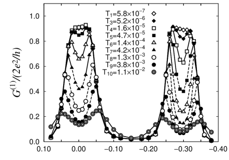
Fig.  3: The temperature dependence of the conductance as a function of the parameter $\varepsilon_{\rm d}$ for the THi-1 case. (For the non-degenerate orbital case.) The regions given by broken lines are considered to be the magnetic state and solid lines region are the non-magnetic state (spin singlet state). This classification is done by comparing the temperature and the Kondo temperature estimated from the magnetic excitation spectra. The suffixes for the temperature are chosen to be common throughout §2.3.1 and Fig. 11 in §3.

Let us see Fig. 3 from high temperature side. There are four peaks at the potentials $\varepsilon_{\rm d}\sim 0.05,-0.05,-0.25$ and $-0.35$ in high temperature region $T\mathrel{\mathchoice{\lower 2.58334pt\vbox{\halign{$\m@th\displaystyle\hfil#\hfil$\cr>\crcr\sim\crcr}}}{\lower 2.58334pt\vbox{\halign{$\m@th\textstyle\hfil#\hfil$\cr>\crcr\sim\crcr}}}{\lower 2.58334pt\vbox{\halign{$\m@th\scriptstyle\hfil#\hfil$\cr>\crcr\sim\crcr}}}{\lower 2.58334pt\vbox{\halign{$\m@th\scriptscriptstyle\hfil#\hfil$\cr>\crcr\sim\crcr}}}}10^{-3}$. These structures correspond to the usual Coulomb oscillations, because the each potential coincides with the point at which the electron number in the dot changes. The thermally broadened peak structures in $T_{10}=1.1\times 10^{-2}$ case change to more sharp peak structures in $T_{9}=3.8\times 10^{-3}$ case. When the temperature gradually decreases below about $T\sim 10^{-3}$, the conductance grows up in the regions $t-U\mathrel{\mathchoice{\lower 2.58334pt\vbox{\halign{$\m@th\displaystyle\hfil#\hfil$\cr<\crcr\sim\crcr}}}{\lower 2.58334pt\vbox{\halign{$\m@th\textstyle\hfil#\hfil$\cr<\crcr\sim\crcr}}}{\lower 2.58334pt\vbox{\halign{$\m@th\scriptstyle\hfil#\hfil$\cr<\crcr\sim\crcr}}}{\lower 2.58334pt\vbox{\halign{$\m@th\scriptscriptstyle\hfil#\hfil$\cr<\crcr\sim\crcr}}}}\varepsilon_{\rm d}\mathrel{\mathchoice{\lower 2.58334pt\vbox{\halign{$\m@th\displaystyle\hfil#\hfil$\cr<\crcr\sim\crcr}}}{\lower 2.58334pt\vbox{\halign{$\m@th\textstyle\hfil#\hfil$\cr<\crcr\sim\crcr}}}{\lower 2.58334pt\vbox{\halign{$\m@th\scriptstyle\hfil#\hfil$\cr<\crcr\sim\crcr}}}{\lower 2.58334pt\vbox{\halign{$\m@th\scriptscriptstyle\hfil#\hfil$\cr<\crcr\sim\crcr}}}}t$ and $-t-3U\mathrel{\mathchoice{\lower 2.58334pt\vbox{\halign{$\m@th\displaystyle\hfil#\hfil$\cr<\crcr\sim\crcr}}}{\lower 2.58334pt\vbox{\halign{$\m@th\textstyle\hfil#\hfil$\cr<\crcr\sim\crcr}}}{\lower 2.58334pt\vbox{\halign{$\m@th\scriptstyle\hfil#\hfil$\cr<\crcr\sim\crcr}}}{\lower 2.58334pt\vbox{\halign{$\m@th\scriptscriptstyle\hfil#\hfil$\cr<\crcr\sim\crcr}}}}\varepsilon_{\rm d}\mathrel{\mathchoice{\lower 2.58334pt\vbox{\halign{$\m@th\displaystyle\hfil#\hfil$\cr<\crcr\sim\crcr}}}{\lower 2.58334pt\vbox{\halign{$\m@th\textstyle\hfil#\hfil$\cr<\crcr\sim\crcr}}}{\lower 2.58334pt\vbox{\halign{$\m@th\scriptstyle\hfil#\hfil$\cr<\crcr\sim\crcr}}}{\lower 2.58334pt\vbox{\halign{$\m@th\scriptscriptstyle\hfil#\hfil$\cr<\crcr\sim\crcr}}}}-t-2U$. The pairs of the peaks at high temperatures in the each region gradually change to the one peak structures. In the lowest temperature limit $T\mathrel{\mathchoice{\lower 2.58334pt\vbox{\halign{$\m@th\displaystyle\hfil#\hfil$\cr<\crcr\sim\crcr}}}{\lower 2.58334pt\vbox{\halign{$\m@th\textstyle\hfil#\hfil$\cr<\crcr\sim\crcr}}}{\lower 2.58334pt\vbox{\halign{$\m@th\scriptstyle\hfil#\hfil$\cr<\crcr\sim\crcr}}}{\lower 2.58334pt\vbox{\halign{$\m@th\scriptscriptstyle\hfil#\hfil$\cr<\crcr\sim\crcr}}}}10^{-6}$, the conductance $G^{(1)}$ coincides to $G_{\rm F}^{(1)}$ in Fig. 2 except the numerical errors brought by the calculation of $P^{{}^{\prime\prime}}(\omega)/\omega$ with NRG method. (From comparison of the conductance $G_{\rm F}^{(1)}$ in Fig. 2 and $G^{(1)}$ at $T_{1}=5.8\times 10^{-7}$ in Fig. 3, $G^{(1)}$ has about $15{\%}$ smaller magnitude at $\varepsilon_{\rm d}=-0.30$. This accuracy of the conductance through the calculation of $P^{{}^{\prime\prime}}(\omega)/\omega$ is not so good in a quantitative sense, but seems to be sufficient to extract the qualitative temperature dependence caused by the change of the electronic state.) As shown later, the Kondo temperature $T_{\rm K}$ strongly depends on $\varepsilon_{\rm d}$. Hereafter, we denote $T_{\rm K}^{*}$ as the lowest Kondo temperature when the potential $\varepsilon_{\rm d}$ is changed. It is estimated to be about $T_{\rm K}^{*}=2.7\times 10^{-5}$ for $\varepsilon_{\rm d}=-0.30$ case, which is near $T_{4}=1.6\times 10^{-5}$ in Fig. 3. The valley of the conductance at $\varepsilon_{\rm d}=-0.30$ becomes very shallow in the cases $T\mathrel{\mathchoice{\lower 2.58334pt\vbox{\halign{$\m@th\displaystyle\hfil#\hfil$\cr<\crcr\sim\crcr}}}{\lower 2.58334pt\vbox{\halign{$\m@th\textstyle\hfil#\hfil$\cr<\crcr\sim\crcr}}}{\lower 2.58334pt\vbox{\halign{$\m@th\scriptstyle\hfil#\hfil$\cr<\crcr\sim\crcr}}}{\lower 2.58334pt\vbox{\halign{$\m@th\scriptscriptstyle\hfil#\hfil$\cr<\crcr\sim\crcr}}}}T_{3}\sim 0.2T_{\rm K}^{*}$. The conductance changes from the usual Coulomb oscillations type to the Kondo resonance type at about $T\sim 0.2T_{\rm K}^{*}$. In the non-degenerate orbital case of this subsection, the interference between tunneling processes via the even and odd orbital channels seems to be not so operative. We expect that the temperature dependence of the growing up of the pair peaks to the flat one peak is almost identical to that of the single orbital case.

Next we present the excitation spectra in detail. Hereafter in this subsection, we mainly discuss only the region $\varepsilon_{\rm d}\leq-3U/2=-0.15$. In this case the Kondo effect of the odd channel electron is important. We have calculated the single particle excitation spectra for the even and the odd orbitals, $\rho_{p}(\omega)$ ($p={\rm e,o}$), which are given as follows,

$$\rho_{p}(\omega) \equiv \frac{1}{Z}\sum_{n,m}\left({\rm e}^{-\beta E_{m}}-{\rm e}^{-\beta E_{n}}\right)$$ (2.11)

$$\times\left(\left|\langle n|d_{p}^{\dagger}|m\rangle\right|^{2}\delta\left(\omega-\left(E_{n}-E_{m}\right)\right)\right.$$

$$\left.+\left|\langle n|d_{p}|m\rangle\right|^{2}\delta\left(\omega+\left(E_{n}-E_{m}\right)\right)\right).$$

The single particle excitation spectra at several temperatures for the case of $\varepsilon_{\rm d}=-0.30$ are shown in Fig. 2.3.1.

[htb]

The single particle excitation spectra at several temperatures for the potential $\varepsilon_{\rm d}=-0.30$ ($\langle n_{\rm o}\rangle\sim 1.0$, in which the odd channel is the Kondo regime). The results are for the non-degenerate orbital case. The spectra are plotted as a function of the logarithm of the energy except the inset plotted by the energy.

In $\rho_{\rm e}(\omega)$ we have no fine structures near the Fermi energy because the even orbital is almost full-filled. On the other hand the odd orbital is almost half-filled, $\langle n_{\rm o}\rangle\sim 1.0$, $\rho_{\rm o}(\omega)$ has fine structures at low temperatures. The Kondo peak on the Fermi energy gradually grows up in the energy region $|\omega|\mathrel{\mathchoice{\lower 2.58334pt\vbox{\halign{$\m@th\displaystyle\hfil#\hfil$\cr<\crcr\sim\crcr}}}{\lower 2.58334pt\vbox{\halign{$\m@th\textstyle\hfil#\hfil$\cr<\crcr\sim\crcr}}}{\lower 2.58334pt\vbox{\halign{$\m@th\scriptstyle\hfil#\hfil$\cr<\crcr\sim\crcr}}}{\lower 2.58334pt\vbox{\halign{$\m@th\scriptscriptstyle\hfil#\hfil$\cr<\crcr\sim\crcr}}}}10^{-4}$ as temperature decreases from $T\sim 10^{-4}$. Growing up of the Kondo peak completes at about $T\mathrel{\mathchoice{\lower 2.58334pt\vbox{\halign{$\m@th\displaystyle\hfil#\hfil$\cr<\crcr\sim\crcr}}}{\lower 2.58334pt\vbox{\halign{$\m@th\textstyle\hfil#\hfil$\cr<\crcr\sim\crcr}}}{\lower 2.58334pt\vbox{\halign{$\m@th\scriptstyle\hfil#\hfil$\cr<\crcr\sim\crcr}}}{\lower 2.58334pt\vbox{\halign{$\m@th\scriptscriptstyle\hfil#\hfil$\cr<\crcr\sim\crcr}}}}10^{-6}$. Reflecting these facts, the conductance near $\varepsilon_{\rm d}\sim-0.30$ increases as temperature decreases. The odd channel seems to be in the Kondo regime. In Fig. 2.3.1 the potential is raised to $\varepsilon_{\rm d}=-0.26$ so that the odd channel is in the mixed valence regime ($\langle n_{\rm o}\rangle\sim 0.8$).

[htb]

The single particle excitation spectra at several temperatures for the potential $\varepsilon_{\rm d}=-0.26$ ($\langle n_{\rm o}\rangle\sim 0.8$). The results are for the non-degenerate orbital case. In this case the odd channel is in the mixed valence regime.

In $\rho_{\rm o}(\omega)$, we can see an excitation peak near $\omega\sim-0.01$ in the case of $T_{10}=1.1\times 10^{-2}$. This corresponds to the excitation from the $N_{\rm o}=1$ state to the $N_{\rm o}=0$ state. As the temperature decreases gradually, the peak position shifts to the Fermi energy, and the peak height increases. It grows up completely in the temperature region $T\mathrel{\mathchoice{\lower 2.58334pt\vbox{\halign{$\m@th\displaystyle\hfil#\hfil$\cr<\crcr\sim\crcr}}}{\lower 2.58334pt\vbox{\halign{$\m@th\textstyle\hfil#\hfil$\cr<\crcr\sim\crcr}}}{\lower 2.58334pt\vbox{\halign{$\m@th\scriptstyle\hfil#\hfil$\cr<\crcr\sim\crcr}}}{\lower 2.58334pt\vbox{\halign{$\m@th\scriptscriptstyle\hfil#\hfil$\cr<\crcr\sim\crcr}}}}10^{-4}$, and has structures seem to be a composite of the two components: the electron excitation of $N_{\rm o}=1\rightarrow N_{\rm o}=0$ and the Kondo peak. As seen in Fig. 2.3.1, these two components are separated with each other when the system is in the Kondo regime. Any way, the intensity of $\rho_{\rm o}(\omega)$ on the Fermi energy increases as temperature decreases, and causes the growth of the conductance in the potential region $-t-3U\mathrel{\mathchoice{\lower 2.58334pt\vbox{\halign{$\m@th\displaystyle\hfil#\hfil$\cr<\crcr\sim\crcr}}}{\lower 2.58334pt\vbox{\halign{$\m@th\textstyle\hfil#\hfil$\cr<\crcr\sim\crcr}}}{\lower 2.58334pt\vbox{\halign{$\m@th\scriptstyle\hfil#\hfil$\cr<\crcr\sim\crcr}}}{\lower 2.58334pt\vbox{\halign{$\m@th\scriptscriptstyle\hfil#\hfil$\cr<\crcr\sim\crcr}}}}\varepsilon_{\rm d}\mathrel{\mathchoice{\lower 2.58334pt\vbox{\halign{$\m@th\displaystyle\hfil#\hfil$\cr<\crcr\sim\crcr}}}{\lower 2.58334pt\vbox{\halign{$\m@th\textstyle\hfil#\hfil$\cr<\crcr\sim\crcr}}}{\lower 2.58334pt\vbox{\halign{$\m@th\scriptstyle\hfil#\hfil$\cr<\crcr\sim\crcr}}}{\lower 2.58334pt\vbox{\halign{$\m@th\scriptscriptstyle\hfil#\hfil$\cr<\crcr\sim\crcr}}}}-t-2U$.

As seen from comparison of Fig. 2.3.1 and Fig. 2.3.1, the Kondo temperature is different in each potential case. To see this point clearly we calculate the magnetic excitation spectrum at zero temperature, $\chi_{\rm m}^{{}^{\prime\prime}}(\omega)$,

$$\chi_{\rm m}^{{}^{\prime\prime}}(\omega) \equiv \sum_{n}\sum_{{\rm Gr}}\left|\langle n\left|\left(S_{{\rm e},z}+S_{{\rm o},z}\right)\right|{\rm Gr}\rangle\right|^{2}$$ (2.12)

$$\times\delta\left(\omega-\left(E_{n}-E_{{\rm Gr}}\right)\right),$$

where $S_{p,z}=(d_{p,\uparrow}^{\dagger}d_{p,\uparrow}-d_{p,\downarrow}^{\dagger}d_{p,\downarrow})/2$ is the spin operator on the $p$-th orbital and ${\rm Gr}$ denotes the ground state of the system. The peak position of the magnetic excitation reflects the characteristic energy of the spin fluctuation. The Kondo temperature $T_{\rm K}$ is defined as the energy of the peak position. ${}^{\hbox{\immediate{?},\penalty 1000\hskip 0.91003pt plus 0.70004pt minus 0.70004pt{\bf{?}})}}$ It is shown in Fig. 4 as a function of the potential $\varepsilon_{\rm d}$, and has the sharp local minima at $\varepsilon_{\rm d}=-0.30$ (where $\langle n_{\rm o}\rangle\sim 1.0$) and $\varepsilon_{\rm d}=0.00$ ($\langle n_{\rm e}\rangle\sim 1.0$).

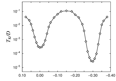
Fig.  4: The Kondo temperature as a function of the potential $\varepsilon_{\rm d}$ for the non-degenerate orbital case.

These minima characterize the temperature at which the conductance behavior changes from the Coulomb oscillations type to the Kondo resonance type.

We point out that the Kondo temperature is also very sensitive to the change of the hybridization $\Delta$ as seen from comparison of the $T_{\rm K}(\varepsilon_{\rm d}=-0.30)=2.7\times 10^{-5}$ ($\Delta_{\rm o}=0.002\pi$) and $T_{\rm K}(\varepsilon_{\rm d}=0.00)=2.7\times 10^{-4}$ ($\Delta_{\rm e}=0.003\pi$), or from the analytical expression for the Kondo temperature. ($T_{\rm K}=\sqrt{U\Delta/2}\exp{[-(\pi U)/(8\Delta)+\Delta/(2U)]}$ for the single orbital impurity Anderson model in the electron-hole symmetric case ${}^{\hbox{\immediate{\bf{?}})}}$). This means that the Kondo temperature of the quantum dot systems is sensitive to the effective distance between leads and dot.

2.3.2 Degenerate orbital case

Next, we consider the situation that the two orbitals have degenerate energy levels. Even if the orbital energies are not degenerate in the strict sense, they should be considered as to be degenerate when the energy difference $\Delta\varepsilon_{\rm d}$ is less than $T_{\rm K}$. (See in Appendix.) The effect of spin fluctuation will appear even when electron number in the dot is even. In this subsection, we present the numerical results for the degenerate orbital case. The parameters are chosen as $\Delta_{\rm e}=0.003\pi$, $\Delta_{\rm o}=0.002\pi$, $\Delta\varepsilon_{\rm d}(=2t)=0$, $U=0.1$ and $J_{\rm H}=0$ for numerical calculation.

The electron occupation numbers for the even and the odd orbitals increase almost simultaneously when the potential $\varepsilon_{\rm d}$ is dropped as shown in Fig. 5.

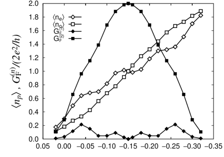
Fig.  5: The expectation value of the electron occupation numbers $\langle n_{p}\rangle$ for the even ($p={\rm e}$) and the odd ($p={\rm o}$) orbitals, and the conductance $G_{\rm F}^{(n)}$ for the THi case ($n=1$) and the THii case ($n=2$), as a function of the potential $\varepsilon_{\rm d}$ at $T=0$ for the degenerate orbital case.

Small but finite difference of the occupation numbers $\langle n_{\rm e}\rangle-\langle n_{\rm o}\rangle$ is caused by the difference between $\Delta_{\rm e}$ and $\Delta_{\rm o}$. The two regions, $\langle n_{\rm e}\rangle>\langle n_{\rm o}\rangle$ and $\langle n_{\rm e}\rangle<\langle n_{\rm o}\rangle$, are separated at $\varepsilon_{\rm d}=-0.15$ because the effective energy levels of the even and the odd orbitals coincide at this point. Conductance at zero temperature, $G_{\rm F}^{(1)}$, is also presented in Fig. 5, and is small in all region, especially near the potential $\varepsilon_{\rm d}\sim-0.15$ since $\langle n_{\rm e}\rangle-\langle n_{\rm o}\rangle$ is small. We note that the factor $\langle n_{\rm e}\rangle-\langle n_{\rm o}\rangle$ in eq. (2.10) is caused by the interference between the tunneling processes via the even and the odd orbitals. The result at $T=0$ is contrasted with the non-degenerate orbital case shown in §2.3.1, and is also contrasted with $G_{\rm F}^{(2)}$ for the case of THii which will be discussed in §3.

Next, we present the temperature dependence of the conductance in Fig. 6. The single particle excitation spectra for the potential $\varepsilon_{\rm d}=-0.15$ ($\langle n_{\rm e}\rangle+\langle n_{\rm o}\rangle=2.0$) are shown in Fig. 2.3.2, and the Kondo temperature as a function of the potential $\varepsilon_{\rm d}$ is also shown in Fig. 7.

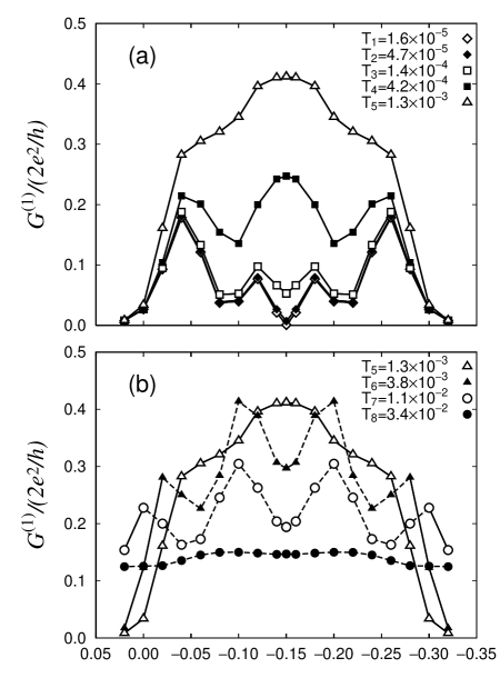
Fig.  6: The temperature dependence of the conductance as a function of the parameter $\varepsilon_{\rm d}$ for the THi-2 case. (For the degenerate orbital case.) The regions given by broken lines are the magnetic state and solid lines region are the non-magnetic state (spin singlet state). The suffixes for the temperature are common throughout §2.3.2 and Fig. 12 in §3.

[htb]

The single particle excitation spectra at several temperatures for the potential $\varepsilon_{\rm d}=-0.15$ ($\langle n_{\rm e}\rangle=\langle n_{\rm o}\rangle=1.0$). The results are for the degenerate orbital case.

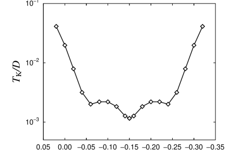
Fig.  7: The Kondo temperature as a function of the potential $\varepsilon_{\rm d}$ for the degenerate orbital case.

In high temperature region (for example $T_{7}=1.1\times 10^{-2}$) of Fig. 6, there are the Coulomb oscillations peaks near $\varepsilon_{\rm d}\sim 0.00,-0.10,-0.20$ and $-0.30$, which correspond to cross points of energies of states with different electron numbers; $\varepsilon_{\rm d}\sim 0,-U,-2U$ and $-3U$, respectively. When the temperature gradually falls down, the conductance in the potential region $-3U\mathrel{\mathchoice{\lower 2.58334pt\vbox{\halign{$\m@th\displaystyle\hfil#\hfil$\cr<\crcr\sim\crcr}}}{\lower 2.58334pt\vbox{\halign{$\m@th\textstyle\hfil#\hfil$\cr<\crcr\sim\crcr}}}{\lower 2.58334pt\vbox{\halign{$\m@th\scriptstyle\hfil#\hfil$\cr<\crcr\sim\crcr}}}{\lower 2.58334pt\vbox{\halign{$\m@th\scriptscriptstyle\hfil#\hfil$\cr<\crcr\sim\crcr}}}}\varepsilon_{\rm d}\mathrel{\mathchoice{\lower 2.58334pt\vbox{\halign{$\m@th\displaystyle\hfil#\hfil$\cr<\crcr\sim\crcr}}}{\lower 2.58334pt\vbox{\halign{$\m@th\textstyle\hfil#\hfil$\cr<\crcr\sim\crcr}}}{\lower 2.58334pt\vbox{\halign{$\m@th\scriptstyle\hfil#\hfil$\cr<\crcr\sim\crcr}}}{\lower 2.58334pt\vbox{\halign{$\m@th\scriptscriptstyle\hfil#\hfil$\cr<\crcr\sim\crcr}}}}0$ once increases, and then decreases to approach to $G_{\rm F}^{(1)}$ at $T=0$. This up-and-down behavior of the conductance with decreasing temperature seems to reflect the partial growth of the coherency in each orbital channel. For example at $T=T_{5}$, the peak height of the Kondo resonance in even channel is about $60\%$ of that of the $T=0$ limit while $50\%$ in odd channel as seen from Fig. 2.3.2. We note the relation, $T_{5}=1.3\times 10^{-3}\sim T_{\rm K}^{*}\equiv T_{\rm K}(\varepsilon_{\rm d}=-0.15)=1.2\times 10^{-3}$. When the temperature decreases below the Kondo temperature, the interference cancellation between the even and the odd orbital channels becomes gradually complete, and the conductance decreases to approach to $G_{\rm F}^{(1)}$. At about $T\mathrel{\mathchoice{\lower 2.58334pt\vbox{\halign{$\m@th\displaystyle\hfil#\hfil$\cr<\crcr\sim\crcr}}}{\lower 2.58334pt\vbox{\halign{$\m@th\textstyle\hfil#\hfil$\cr<\crcr\sim\crcr}}}{\lower 2.58334pt\vbox{\halign{$\m@th\scriptstyle\hfil#\hfil$\cr<\crcr\sim\crcr}}}{\lower 2.58334pt\vbox{\halign{$\m@th\scriptscriptstyle\hfil#\hfil$\cr<\crcr\sim\crcr}}}}T_{3}=1.4\times 10^{-4}\sim 0.1T_{\rm K}^{*}$, the conductance reaches to the low temperature limit. We have weak four peak structures in $G_{\rm F}^{(1)}$, but the peak positions do not coincide with those of the Coulomb oscillations.

We note that the minimum of the Kondo temperature, $T_{\rm K}^{*}$, is much higher than that of the non-degenerate orbital case presented in the previous subsection, even though the hybridization strengths are same. This behavior has been recognized in the 4-fold degeneracy cases of the impurity Anderson model where the parameters satisfy $\Delta_{\rm e}=\Delta_{\rm o}$. ${}^{\hbox{\immediate{?},\penalty 1000\hskip 0.91003pt plus 0.70004pt minus 0.70004pt{\bf{?}})}}$

2.3.3 Effect of Hund’s rule coupling

The energy splitting due to Hund’s rule coupling has been observed in the quantum dot which have high geometrical symmetry. ${}^{\hbox{\immediate{?})}}$ This coupling brings the triplet spin state for the two electrons configuration of the dot. The Kondo temperature would be strongly reduced because the hybridization processes are restricted in this case. ${}^{\hbox{\immediate{\bf{?}})}}$ In this subsection the numerical results for the presence of Hund’s rule coupling are shown. We choose the parameters $\Delta_{\rm e}=0.003\pi$, $\Delta_{\rm o}=0.002\pi$, $\Delta\varepsilon_{\rm d}=0$, $U=0.1$ and $J_{\rm H}=0.020$.

The numerical results of $\langle n_{p}\rangle$ and $G_{\rm F}^{(1)}$ as a function of the potential $\varepsilon_{\rm d}$ are shown in Fig. 8.

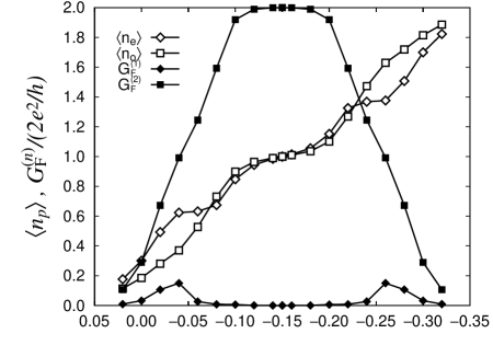
Fig.  8: The expectation value of the electron occupation numbers $\langle n_{p}\rangle$ for the even ($p={\rm e}$) and the odd ($p={\rm o}$) orbital, and the conductance $G_{\rm F}^{(n)}$ for the THi case ($n=1$) and the THii case ($n=2$), as a function of the potential $\varepsilon_{\rm d}$ at $T=0$ for the presence of Hund’s rule coupling case.

When the potential $\varepsilon_{\rm d}$ is dropped, the first electron occupies the dot at $\varepsilon_{\rm d}\sim 0.00$ ($\langle n_{\rm e}\rangle+\langle n_{\rm o}\rangle\sim 0.5$), the second electron at $\varepsilon_{\rm d}\sim-U+\left|J_{\rm H}\right|=-0.08$ ($\langle n_{\rm e}\rangle+\langle n_{\rm o}\rangle\sim 1.5$), the third electron at $\varepsilon_{\rm d}\sim-2U-\left|J_{\rm H}\right|=-0.22$ ($\langle n_{\rm e}\rangle+\langle n_{\rm o}\rangle\sim 2.5$), and the forth electron at $\varepsilon_{\rm d}\sim-3U=-0.30$ ($\langle n_{\rm e}\rangle+\langle n_{\rm o}\rangle\sim 3.5$). (The potential values at $\varepsilon_{\rm d}=0,-U+\left|J_{\rm H}\right|,-2U-\left|J_{\rm H}\right|$ and $-3U$ are the cross points of the energies of the states with different electron number without the hybridization term.) The difference of the occupation numbers $\langle n_{\rm e}\rangle-\langle n_{\rm o}\rangle$ is brought from the difference of the hybridization strengths as previously noted. The way of the electrons occupancy and the behavior of the conductance as a function of the potential $\varepsilon_{\rm d}$ at zero temperature, $G_{\rm F}^{(1)}$, are roughly similar to that of the case shown in §2.3.2, in which Hund’s rule coupling energy is neglected. But the effect of Hund’s rule coupling can be recognized in the potential region $-2U-\left|J_{\rm H}\right|\mathrel{\mathchoice{\lower 2.58334pt\vbox{\halign{$\m@th\displaystyle\hfil#\hfil$\cr<\crcr\sim\crcr}}}{\lower 2.58334pt\vbox{\halign{$\m@th\textstyle\hfil#\hfil$\cr<\crcr\sim\crcr}}}{\lower 2.58334pt\vbox{\halign{$\m@th\scriptstyle\hfil#\hfil$\cr<\crcr\sim\crcr}}}{\lower 2.58334pt\vbox{\halign{$\m@th\scriptscriptstyle\hfil#\hfil$\cr<\crcr\sim\crcr}}}}\varepsilon_{\rm d}\mathrel{\mathchoice{\lower 2.58334pt\vbox{\halign{$\m@th\displaystyle\hfil#\hfil$\cr<\crcr\sim\crcr}}}{\lower 2.58334pt\vbox{\halign{$\m@th\textstyle\hfil#\hfil$\cr<\crcr\sim\crcr}}}{\lower 2.58334pt\vbox{\halign{$\m@th\scriptstyle\hfil#\hfil$\cr<\crcr\sim\crcr}}}{\lower 2.58334pt\vbox{\halign{$\m@th\scriptscriptstyle\hfil#\hfil$\cr<\crcr\sim\crcr}}}}-U+\left|J_{\rm H}\right|$ (where $\langle n_{\rm e}\rangle+\langle n_{\rm o}\rangle\sim 2.0$). The difference of the occupation number between the even and the odd orbitals $\langle n_{\rm e}\rangle-\langle n_{\rm o}\rangle$ is suppressed compared with the results in §2.3.2. Therefore the conductance at zero temperature, $G_{\rm F}^{(1)}$, is very small in the potential region where the interference cancellation occurs.

The temperature dependence of the conductance is presented in Fig. 9.

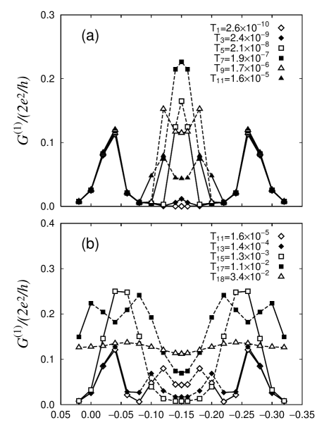
Fig.  9: The temperature dependence of the conductance as a function of the parameter $\varepsilon_{\rm d}$ for the THii-3 case. (Hund’s rule coupling case.) The regions given by broken lines are the magnetic state and solid lines region are the non-magnetic state (spin singlet state). The suffixes for the temperature are common throughout §2.3.3 and Fig. 13 in §3.

The single particle excitation spectra at the potential $\varepsilon_{\rm d}=-0.15$ ($\langle n_{\rm e}\rangle+\langle n_{\rm o}\rangle=2.0$) are shown in Fig. 2.3.3, and the Kondo temperature as a function of the potential $\varepsilon_{\rm d}$ is shown in Fig. 10.

[htb]

The single particle excitation spectra at several temperatures for the potential $\varepsilon_{\rm d}=-0.15$ ($\langle n_{\rm e}\rangle+\langle n_{\rm o}\rangle=2.0$). The results are for the presence of Hund’s rule coupling case.

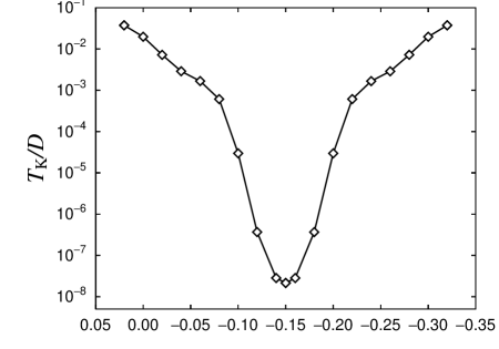
Fig.  10: The Kondo temperature as a function of the potential $\varepsilon_{\rm d}$ for the presence of Hund’s rule coupling case.

The Kondo temperature in the region $-2U-\left|J_{\rm H}\right|\mathrel{\mathchoice{\lower 2.58334pt\vbox{\halign{$\m@th\displaystyle\hfil#\hfil$\cr<\crcr\sim\crcr}}}{\lower 2.58334pt\vbox{\halign{$\m@th\textstyle\hfil#\hfil$\cr<\crcr\sim\crcr}}}{\lower 2.58334pt\vbox{\halign{$\m@th\scriptstyle\hfil#\hfil$\cr<\crcr\sim\crcr}}}{\lower 2.58334pt\vbox{\halign{$\m@th\scriptscriptstyle\hfil#\hfil$\cr<\crcr\sim\crcr}}}}\varepsilon_{\rm d}\mathrel{\mathchoice{\lower 2.58334pt\vbox{\halign{$\m@th\displaystyle\hfil#\hfil$\cr<\crcr\sim\crcr}}}{\lower 2.58334pt\vbox{\halign{$\m@th\textstyle\hfil#\hfil$\cr<\crcr\sim\crcr}}}{\lower 2.58334pt\vbox{\halign{$\m@th\scriptstyle\hfil#\hfil$\cr<\crcr\sim\crcr}}}{\lower 2.58334pt\vbox{\halign{$\m@th\scriptscriptstyle\hfil#\hfil$\cr<\crcr\sim\crcr}}}}-U+\left|J_{\rm H}\right|$ is far less than that shown in Fig. 7. This small $T_{\rm K}$ is caused by the reduction of the hybridization processes due to Hund’s rule coupling which restricts the two electrons states in the dot to be the triplet state.

In high temperature region (for example $T_{17}=1.1\times 10^{-2}$) of Fig. 9, there are the Coulomb oscillations at $\varepsilon_{\rm d}\sim 0.00,-0.08,-0.22$ and $\varepsilon_{\rm d}\sim-0.30$. The conductance approaches to $G_{\rm F}^{(1)}$ at about $T\sim T_{3}\sim 0.1T_{\rm K}^{*}$ ($T_{\rm K}^{*}\equiv T_{\rm K}(\varepsilon_{\rm d}=-0.15)=2.1\times 10^{-8}$).

We compare the results in Fig. 9 with those in Fig. 6. The conductance in the two cases shows almost identical behavior in the region $\varepsilon_{\rm d}\mathrel{\mathchoice{\lower 2.58334pt\vbox{\halign{$\m@th\displaystyle\hfil#\hfil$\cr>\crcr\sim\crcr}}}{\lower 2.58334pt\vbox{\halign{$\m@th\textstyle\hfil#\hfil$\cr>\crcr\sim\crcr}}}{\lower 2.58334pt\vbox{\halign{$\m@th\scriptstyle\hfil#\hfil$\cr>\crcr\sim\crcr}}}{\lower 2.58334pt\vbox{\halign{$\m@th\scriptscriptstyle\hfil#\hfil$\cr>\crcr\sim\crcr}}}}-U+\left|J_{\rm H}\right|=-0.08$ and $\varepsilon_{\rm d}\mathrel{\mathchoice{\lower 2.58334pt\vbox{\halign{$\m@th\displaystyle\hfil#\hfil$\cr<\crcr\sim\crcr}}}{\lower 2.58334pt\vbox{\halign{$\m@th\textstyle\hfil#\hfil$\cr<\crcr\sim\crcr}}}{\lower 2.58334pt\vbox{\halign{$\m@th\scriptstyle\hfil#\hfil$\cr<\crcr\sim\crcr}}}{\lower 2.58334pt\vbox{\halign{$\m@th\scriptscriptstyle\hfil#\hfil$\cr<\crcr\sim\crcr}}}}-2U-\left|J_{\rm H}\right|=-0.22$. They reach to the lowest temperature behavior for $T\mathrel{\mathchoice{\lower 2.58334pt\vbox{\halign{$\m@th\displaystyle\hfil#\hfil$\cr<\crcr\sim\crcr}}}{\lower 2.58334pt\vbox{\halign{$\m@th\textstyle\hfil#\hfil$\cr<\crcr\sim\crcr}}}{\lower 2.58334pt\vbox{\halign{$\m@th\scriptstyle\hfil#\hfil$\cr<\crcr\sim\crcr}}}{\lower 2.58334pt\vbox{\halign{$\m@th\scriptscriptstyle\hfil#\hfil$\cr<\crcr\sim\crcr}}}}10^{-4}$ in that region. In the region $-2U-\left|J_{\rm H}\right|\mathrel{\mathchoice{\lower 2.58334pt\vbox{\halign{$\m@th\displaystyle\hfil#\hfil$\cr<\crcr\sim\crcr}}}{\lower 2.58334pt\vbox{\halign{$\m@th\textstyle\hfil#\hfil$\cr<\crcr\sim\crcr}}}{\lower 2.58334pt\vbox{\halign{$\m@th\scriptstyle\hfil#\hfil$\cr<\crcr\sim\crcr}}}{\lower 2.58334pt\vbox{\halign{$\m@th\scriptscriptstyle\hfil#\hfil$\cr<\crcr\sim\crcr}}}}\varepsilon_{\rm d}\mathrel{\mathchoice{\lower 2.58334pt\vbox{\halign{$\m@th\displaystyle\hfil#\hfil$\cr<\crcr\sim\crcr}}}{\lower 2.58334pt\vbox{\halign{$\m@th\textstyle\hfil#\hfil$\cr<\crcr\sim\crcr}}}{\lower 2.58334pt\vbox{\halign{$\m@th\scriptstyle\hfil#\hfil$\cr<\crcr\sim\crcr}}}{\lower 2.58334pt\vbox{\halign{$\m@th\scriptscriptstyle\hfil#\hfil$\cr<\crcr\sim\crcr}}}}-U+\left|J_{\rm H}\right|$ in Fig. 9, the conductance initially increases with decreasing temperature, and then it decreases in the very low temperature. This behavior is similar to the up-and-down behavior in the region of $-2U\mathrel{\mathchoice{\lower 2.58334pt\vbox{\halign{$\m@th\displaystyle\hfil#\hfil$\cr<\crcr\sim\crcr}}}{\lower 2.58334pt\vbox{\halign{$\m@th\textstyle\hfil#\hfil$\cr<\crcr\sim\crcr}}}{\lower 2.58334pt\vbox{\halign{$\m@th\scriptstyle\hfil#\hfil$\cr<\crcr\sim\crcr}}}{\lower 2.58334pt\vbox{\halign{$\m@th\scriptscriptstyle\hfil#\hfil$\cr<\crcr\sim\crcr}}}}\varepsilon_{\rm d}\mathrel{\mathchoice{\lower 2.58334pt\vbox{\halign{$\m@th\displaystyle\hfil#\hfil$\cr<\crcr\sim\crcr}}}{\lower 2.58334pt\vbox{\halign{$\m@th\textstyle\hfil#\hfil$\cr<\crcr\sim\crcr}}}{\lower 2.58334pt\vbox{\halign{$\m@th\scriptstyle\hfil#\hfil$\cr<\crcr\sim\crcr}}}{\lower 2.58334pt\vbox{\halign{$\m@th\scriptscriptstyle\hfil#\hfil$\cr<\crcr\sim\crcr}}}}-U$ in Fig. 6. However in the present case, the temperature at which the conductance reaches to the lowest temperature behavior is much lower because $T_{\rm K}^{*}$ is very low. The difference of the occupation number is suppressed by Hund’s rule coupling, so the conductance $G_{\rm F}^{(1)}$ in this region becomes almost zero.

The qualitative features of the temperature dependence of the spectra shown in Fig. 2.3.3 are similar to those shown in Fig. 2.3.2 except that the temperature scale of the former is very low. The peak at $\omega\sim 0$ in $\rho_{\rm e}(\omega)$ gradually begins to grow up at about $T\sim 10^{-5}$, while the peak in $\rho_{\rm o}(\omega)$ starts to grow up at about $T\sim 10^{-7}$. The difference of the temperatures at which the Kondo peak starts to grow up in each channel is enhanced by Hund’s rule term, though $\Delta_{\rm e}$ and $\Delta_{\rm o}$ are chosen commonly to those of Fig. 2.3.2. But we note that the peaks reach almost simultaneously to the low temperature limit at about $T\sim 10^{-9}$. The finite conductance value in the temperature region $10^{-7}\mathrel{\mathchoice{\lower 2.58334pt\vbox{\halign{$\m@th\displaystyle\hfil#\hfil$\cr<\crcr\sim\crcr}}}{\lower 2.58334pt\vbox{\halign{$\m@th\textstyle\hfil#\hfil$\cr<\crcr\sim\crcr}}}{\lower 2.58334pt\vbox{\halign{$\m@th\scriptstyle\hfil#\hfil$\cr<\crcr\sim\crcr}}}{\lower 2.58334pt\vbox{\halign{$\m@th\scriptscriptstyle\hfil#\hfil$\cr<\crcr\sim\crcr}}}}T\mathrel{\mathchoice{\lower 2.58334pt\vbox{\halign{$\m@th\displaystyle\hfil#\hfil$\cr<\crcr\sim\crcr}}}{\lower 2.58334pt\vbox{\halign{$\m@th\textstyle\hfil#\hfil$\cr<\crcr\sim\crcr}}}{\lower 2.58334pt\vbox{\halign{$\m@th\scriptstyle\hfil#\hfil$\cr<\crcr\sim\crcr}}}{\lower 2.58334pt\vbox{\halign{$\m@th\scriptscriptstyle\hfil#\hfil$\cr<\crcr\sim\crcr}}}}10^{-5}$ reflects the growth of the peak in the even channel. The decrease of the conductance in $10^{-9}\mathrel{\mathchoice{\lower 2.58334pt\vbox{\halign{$\m@th\displaystyle\hfil#\hfil$\cr<\crcr\sim\crcr}}}{\lower 2.58334pt\vbox{\halign{$\m@th\textstyle\hfil#\hfil$\cr<\crcr\sim\crcr}}}{\lower 2.58334pt\vbox{\halign{$\m@th\scriptstyle\hfil#\hfil$\cr<\crcr\sim\crcr}}}{\lower 2.58334pt\vbox{\halign{$\m@th\scriptscriptstyle\hfil#\hfil$\cr<\crcr\sim\crcr}}}}T\mathrel{\mathchoice{\lower 2.58334pt\vbox{\halign{$\m@th\displaystyle\hfil#\hfil$\cr<\crcr\sim\crcr}}}{\lower 2.58334pt\vbox{\halign{$\m@th\textstyle\hfil#\hfil$\cr<\crcr\sim\crcr}}}{\lower 2.58334pt\vbox{\halign{$\m@th\scriptstyle\hfil#\hfil$\cr<\crcr\sim\crcr}}}{\lower 2.58334pt\vbox{\halign{$\m@th\scriptscriptstyle\hfil#\hfil$\cr<\crcr\sim\crcr}}}}10^{-8}$ reflects the growth of the peak in the odd channel. Hund’s rule coupling prevents to observe the low temperature limit behaviors, but it makes wide an intermediate temperature region where a part of the orbital is affected by the Kondo effect.

3 Two Conduction Channels in Each Lead

In §2, we have discussed the situation classified to the THi that dot’s orbitals hybridize only to one-dimensional degree of freedom in each lead. In this section we consider also the perpendicular components in the leads as the degree of freedoms. We assume that there are two orbitals in the dot, which are even and odd, respectively, under the $zx$ mirror. These are assumed to be even under the $yz$ mirror. We name these orbitals in the dot as the even orbital and the odd orbital, and denote them by $d_{{\rm e}\sigma}$ and $d_{{\rm o}\sigma}$. (Note that in §2, the even and the odd were denoted with respect to the $yz$ plane.) We assume that we have two conduction channels in each lead, which are even and odd, respectively, under the $zx$ mirror. These are named as the even and the odd channels in the left and the right leads. We write them as $c_{{\rm Le}k\sigma}$, $c_{{\rm Lo}k\sigma}$, $c_{{\rm Re}k\sigma}$ and $c_{{\rm Ro}k\sigma}$, respectively. The Hamiltonian $H_{\rm l}$ and $H_{\rm l-d}$ is written as follows;

$$H_{{\rm l}} = \sum_{k\sigma}(\varepsilon_{k}c_{{\rm Le}k\sigma}^{\dagger}c_{{\rm Le}k\sigma}+\varepsilon_{k}c_{{\rm Lo}k\sigma}^{\dagger}c_{{\rm Lo}k\sigma})$$ (3.1)

$$+\sum_{k\sigma}(\varepsilon_{k}c_{{\rm Re}k\sigma}^{\dagger}c_{{\rm Re}k\sigma},+\varepsilon_{k}c_{{\rm Ro}k\sigma}^{\dagger}c_{{\rm Ro}k\sigma}),$$

$$H_{{\rm l-d}} = \frac{1}{\sqrt{2}}\sum_{k\sigma}(V_{\rm e}d_{{\rm e}\sigma}^{\dagger}c_{{\rm Le}k\sigma}+V_{\rm o}d_{{\rm o}\sigma}^{\dagger}c_{{\rm Lo}k\sigma}+{\rm h.c.})$$ (3.2)

$$+\frac{1}{\sqrt{2}}\sum_{k\sigma}(V_{\rm e}d_{{\rm e}\sigma}^{\dagger}c_{{\rm Re}k\sigma}+V_{\rm o}d_{{\rm o}\sigma}^{\dagger}c_{{\rm Ro}k\sigma}+{\rm h.c.}).$$

When the operators, $s_{k\sigma}$ and $a_{k\sigma}$ in eqs. (2.5) and (2.6), are replaced respectively by newly defined ones, $s_{k\sigma}=(c_{{\rm Le}k\sigma}+c_{{\rm Re}k\sigma})/\sqrt{2}$ and $a_{k\sigma}=(c_{{\rm Lo}k\sigma}+c_{{\rm Ro}k\sigma})/\sqrt{2}$, we have the identical form for the Hamiltonian.

But the conductance formula is different from that in §2. We have the situation classified to the THii that the tunneling via the even and the odd channels are independent in the tunneling between leads. The conductance formula is given as follows, ${}^{\hbox{\immediate{\bf{?}})}}$

$$G^{(2)} = \frac{2e^{2}}{h}\sum_{p={\rm e,o}}\int d\varepsilon\left(-\frac{\partial f}{\partial\varepsilon}\right)\pi\Delta_{p}\rho_{p}(\varepsilon).$$ (3.3)

Here $\rho_{p}(\varepsilon)$ is the single particle excitation spectrum of the dot orbital with symmetry $p$. At $T=0$, the conductance formula is reduced to the following expression,

$$G_{\rm F}^{(2)} = \frac{2e^{2}}{h}\sum_{p={\rm e,o}}\sin^{2}\left\{\frac{\pi}{2}\langle n_{p}\rangle\right\}.$$ (3.4)

The numerical calculations are performed for the three cases; (1) non-degenerate orbital case, (2) degenerate orbital case, and (3) presence of Hund’s rule coupling. The parameters are chosen to be same as in §2, for comparison. Then the electronic states of the both systems are identically mapped. The conductance for three cases is shown in Figs. 11, 12 and 13, respectively. (Conductance at $T=0$ has been shown in Figs. 2, 5 and 8, respectively.)

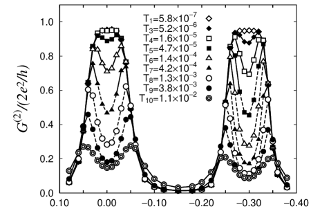
Fig.  11: The temperature dependence of the conductance as a function of the parameter $\varepsilon_{\rm d}$ for the THii-1 case. (Tunneling processes via the even and the odd orbitals are independent. For the non-degenerate orbital case.)

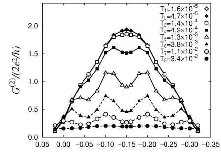
Fig.  12: The temperature dependence of the conductance as a function of the parameter $\varepsilon_{\rm d}$ for the THii-2 case. (For the degenerate orbital case.)

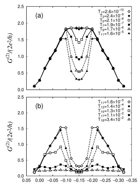
Fig.  13: The temperature dependence of the conductance as a function of the parameter $\varepsilon_{\rm d}$ for the THii-3 case. (Hund’s rule coupling case.)

As note previously, the interference effect of tunneling processes via the even and odd orbitals do not occur in the present THii case. Therefore the phenomena due to the interference in THi case do not appear in the present. Maximum of the intensity at $T=0$ has $2\times 2e^{2}/h$, twice of the unitarity limit value of the single conduction channel case. In Fig. 11, the differences of the conductance behaviors from those of Fig. 3 are not well recognized, because the interference is not so significant in the non-degenerate orbital case.

In Fig. 12 of the degenerate orbital case, the conductance in high temperature region (for example $T_{7}=1.1\times 10^{-2}$) behaves the Coulomb oscillations type similar to that of Fig. 6. As temperature decreases, it increases gradually filling the valley between four peaks. At $T\sim T_{5}=1.3\times 10^{-3}$, the conductance is rather large indicating the partial growing up of the Kondo resonance in each channel. But we do not have the up-and-down behaviors such that shown in Fig. 6. At about $T\mathrel{\mathchoice{\lower 2.58334pt\vbox{\halign{$\m@th\displaystyle\hfil#\hfil$\cr<\crcr\sim\crcr}}}{\lower 2.58334pt\vbox{\halign{$\m@th\textstyle\hfil#\hfil$\cr<\crcr\sim\crcr}}}{\lower 2.58334pt\vbox{\halign{$\m@th\scriptstyle\hfil#\hfil$\cr<\crcr\sim\crcr}}}{\lower 2.58334pt\vbox{\halign{$\m@th\scriptscriptstyle\hfil#\hfil$\cr<\crcr\sim\crcr}}}}T_{3}=1.4\times 10^{-4}\sim 0.1T_{\rm K}^{*}$, the conductance approaches to the low temperature limit which has a broadened peak structure. In Fig. 13, for Hund’s rule coupling case, the conductance behavior is similar to that of the degenerate orbital case. But the conductance in the potential region $\varepsilon_{\rm d}\sim-0.15$ does not increases to the low temperature limit values until the temperature becomes very low, $T\mathrel{\mathchoice{\lower 2.58334pt\vbox{\halign{$\m@th\displaystyle\hfil#\hfil$\cr<\crcr\sim\crcr}}}{\lower 2.58334pt\vbox{\halign{$\m@th\textstyle\hfil#\hfil$\cr<\crcr\sim\crcr}}}{\lower 2.58334pt\vbox{\halign{$\m@th\scriptstyle\hfil#\hfil$\cr<\crcr\sim\crcr}}}{\lower 2.58334pt\vbox{\halign{$\m@th\scriptscriptstyle\hfil#\hfil$\cr<\crcr\sim\crcr}}}}T_{3}=2.4\times 10^{-9}\sim 0.1T_{\rm K}^{*}$. Therefore in the wide temperature range we can see two peak structures similar to that of the non-degenerate orbital case.

4 Summary and Discussion

The Kondo effects in the quantum dot systems have been investigated for the cases that (THi) there is one conduction channel in each lead and the tunneling processes via the different orbitals in the dot interfere each other (in §2), and (THii) there are two conduction channels in each lead but the tunneling processes do not interfere (in §3). In both cases, the following three cases for the orbital degeneracy have been examined; (1) non-degenerate orbital case, (2) degenerate orbital case, and (3) presence of Hund’s rule coupling case. The linear response conductance for the bias voltage has been calculated as a function of the gate voltage. The numerical calculations have been performed in wide temperature range by using NRG method.

The Coulomb oscillations are observed in high temperature region commonly in the all cases, but various types of conductance behavior appear reflecting the growing up of the Kondo resonance at low temperatures. The low temperature limit behaviors appear in the temperature region $T\mathrel{\mathchoice{\lower 2.58334pt\vbox{\halign{$\m@th\displaystyle\hfil#\hfil$\cr<\crcr\sim\crcr}}}{\lower 2.58334pt\vbox{\halign{$\m@th\textstyle\hfil#\hfil$\cr<\crcr\sim\crcr}}}{\lower 2.58334pt\vbox{\halign{$\m@th\scriptstyle\hfil#\hfil$\cr<\crcr\sim\crcr}}}{\lower 2.58334pt\vbox{\halign{$\m@th\scriptscriptstyle\hfil#\hfil$\cr<\crcr\sim\crcr}}}}0.1T_{\rm K}^{*}\sim 0.2T_{\rm K}^{*}$, where $T_{\rm K}^{*}$ is the minimum value of the Kondo temperature when $\varepsilon_{\rm d}$ is changed.

In the non-degenerate orbital cases, THi-1 and THii-1, the pair of the two peaks of the Coulomb oscillations gradually changes one flat peak structure as temperature decreases below $0.2T_{\rm K}^{*}$. The conductance behaviors in these two cases are not so different because the interference effect is not significant.

In the degenerate orbital case of THi-2, the interference cancellation between the tunneling processes via the different orbitals causes small conductance at temperatures below $0.1T_{\rm K}^{*}$. But we have the characteristic up-and-down behavior of the conductance with increasing temperature in the intermediate temperature range. This is caused by the partial destruction of the coherency due to the partial breaking of the Kondo singlet state in each orbital channel. In the case of THi-3 (Hund’s rule coupling), the temperature region where the conductance shows the characteristic behaviors due to such partial destruction of the coherency shifts to low temperature side, because the Kondo temperature is largely reduced.

In Fig. 12 of THii-2 and Fig. 13 of THii-3 in §3, four Coulomb oscillations peaks gradually become one broad peak structure as temperature decreases below $0.1T_{\rm K}^{*}$, because the interference between two channels does not exist. But we have a regime indicating the partial growing up of the Kondo resonance in the intermediate temperature region. In the case of THii-3, we have two peak structures similar to that of the non-degenerate orbital case in wide temperature range.

Electronic states of the cases THi and THii are mapped on with each other, but the tunneling current in low temperatures shows quite different behaviors. The sensitivities of the conductance to the temperature and to the gate voltage are caused by the difference of the Kondo temperature at each potential, are inherent in the interacting systems.

Here we roughly estimate the characteristic temperature by assuming $U\sim 1{\rm meV}(\sim 10{\rm K})$ and $\Delta_{p}\sim 0.1{\rm meV}(\sim 1{\rm K})$. The Kondo temperature $T_{\rm K}^{*}$ is estimated to be about $3{\rm mK}$ ($\Delta_{\rm o}\sim 0.06{\rm meV}$) and $30{\rm mK}$ ($\Delta_{\rm e}\sim 0.1{\rm meV}$) for the case (1), $100{\rm mK}$ for the case (2), and $10^{-3}{\rm mK}$ for the case (3). We note, however, the Kondo temperature is very sensitive to the hybridization strength.

Recently experimental work has been performed with controlling $\Delta$ by Goldhaber-Gordon et al. ${}^{\hbox{\immediate{?})}}$ The change of the conductance due to the Kondo effect seems to appear in their system. The results seem to correspond to our numerical results at higher temperature region shown in Fig. 3 and Fig. 11, $10^{-3}\mathrel{\mathchoice{\lower 2.58334pt\vbox{\halign{$\m@th\displaystyle\hfil#\hfil$\cr<\crcr\sim\crcr}}}{\lower 2.58334pt\vbox{\halign{$\m@th\textstyle\hfil#\hfil$\cr<\crcr\sim\crcr}}}{\lower 2.58334pt\vbox{\halign{$\m@th\scriptstyle\hfil#\hfil$\cr<\crcr\sim\crcr}}}{\lower 2.58334pt\vbox{\halign{$\m@th\scriptscriptstyle\hfil#\hfil$\cr<\crcr\sim\crcr}}}}T\mathrel{\mathchoice{\lower 2.58334pt\vbox{\halign{$\m@th\displaystyle\hfil#\hfil$\cr<\crcr\sim\crcr}}}{\lower 2.58334pt\vbox{\halign{$\m@th\textstyle\hfil#\hfil$\cr<\crcr\sim\crcr}}}{\lower 2.58334pt\vbox{\halign{$\m@th\scriptstyle\hfil#\hfil$\cr<\crcr\sim\crcr}}}{\lower 2.58334pt\vbox{\halign{$\m@th\scriptscriptstyle\hfil#\hfil$\cr<\crcr\sim\crcr}}}}10^{-2}$, qualitatively.

5 Non-Degenerate Orbital to Degenerate Orbital

In §2 and 3, we have used models that the energy separation of the orbitals, $\Delta\varepsilon_{\rm d}$, is extreme. It is large (in §2.3.1 and Fig. 11 in §3) or zero (in §2.3.2, 2.3.3 and Fig. 12, 13 in §3). Here we change gradually $\Delta\varepsilon_{\rm d}$ and study when the low temperature properties changes from the non-degenerate orbital case to the degenerate orbital case. The parameters for the hybridization strength are chosen to satisfy the relations $\Delta_{\rm e}=\Delta_{\rm o}\equiv\Delta$, for simplicity. (For the case of THi, the tunneling current between leads disappears by this setting. But in Appendix, we mainly concentrate on the effects of the energy separation on the Kondo effect.) The parameters are chosen as $\Delta=0.0025\pi$, $U=0.1$ and $J_{\rm H}=0$. The potential depth is fixed at $\varepsilon_{\rm d}=-0.15$, therefore the system is in the electron-hole symmetry. (The electron occupation number in the dot satisfies $\langle n\rangle\equiv\langle n_{\rm e}\rangle+\langle n_{\rm o}\rangle=2$, exactly.)

The electron occupation numbers for the even and the odd orbitals are shown as a function of $\Delta\varepsilon_{\rm d}$ in Fig. 14.

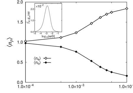
Fig.  14: The electron occupation numbers for the even and the odd orbitals as a function of the orbital energy separation $\Delta\varepsilon_{\rm d}$. Inset figure is the magnetic excitation spectrum at $\varepsilon_{\rm d}=0$, $T=0$. The Kondo temperature at $\Delta\varepsilon_{\rm d}=0$ is estimated to be about $T=1.5\times 10^{-3}$ from the peak position of the spectrum.

As $\Delta\varepsilon_{\rm d}$ increases, difference of the occupation number steeply increases at about $\Delta\varepsilon_{\rm d}\sim 2\times 10^{-3}$ (where $\langle n_{\rm e}\rangle\sim 1.5$ and $\langle n_{\rm o}\rangle\sim 0.5$). The Kondo temperature at $\Delta\varepsilon_{\rm d}=0$ is estimated to be about $T_{\rm K}=1.5\times 10^{-3}$ from the magnetic excitation spectrum shown in the inset of Fig. 14. We may conclude that the cross over occurs at about $\Delta\varepsilon_{\rm d}\sim T_{\rm K}(\Delta\varepsilon_{\rm d}=0)$. We note that $\Delta\varepsilon_{\rm d}$ is much smaller than the hybridization width, $\Delta$.

References

- [1] See for example, A. C. Hewson: The Kondo problem to Heavy Fermions (Cambridge University Press, Cambridge, 1993) and references cited therein.
- [2] T. K. Ng and P. A. Lee: Phys. Rev. Lett. 61 (1988) 1768.
- [3] L. I. Glazman and M. É. Raĭkh: JETP Lett. 47 (1988) 452.
- [4] A. Kawabata: J. Phys. Soc. Jpn. 60 (1991) 3222.
- [5] S. Hershfield, J. H. Davies and J. W. Wilkins: Phys. Rev. Lett. 67 (1991) 3720; S. Hershfield, J. H. Davies and J. W. Wilkins: Phys. Rev. B 46 (1992) 7046.
- [6] A. L. Yeyati, A. Wartín-Rodero and F. Flores: Phys. Rev. Lett. 71 (1993) 2991.
- [7] Y. Meir, N. S. Wingreen and P. A. Lee: Phys. Rev. Lett. 70 (1993) 2601; N. S. Wingreen and Y. Meir: Phys. Rev. B 49 (1994) 11040.
- [8] T. Inoshita, A. Shimizu, Y. Kuramoto and H. Sasaki: Phys. Rev. B 48 (1993) 14725.
- [9] A. Oguri, H. Ishii and T. Saso: Phys. Rev. B 51 (1995) 4715; A. Oguri: Phys. Rev. B 56 (1997) 13422.
- [10] W. Izumida, O. Sakai and Y. Shimizu: J. Phys. Soc. Jpn. 66 (1997) 717.
- [11] D. Goldhaber-Gordon, H. Shtrikman, D. Mahalu, D. Abusch-Magder,U. Meirav, and M. A. Kastner: nature 391 (1998) 156.
- [12] S. Tarucha, D. G. Austing, and T. Honda: Phys. Rev. Lett. 77 (1996) 3613.
- [13] H. R. Krishnamurthy, J. W. Wilkins and K. G. Wilson: Phys. Rev. B 21 (1980) 1003; ibid. 21 (1980) 1044.
- [14] O. Sakai, S. Suzuki and Y. Shimizu: Physica B 206 & 207 (1995) 141.
- [15] Y. Shimizu and O. Sakai: Computational Physics as a New Frontier in Condensed Matter Research ed. H. Takayama, M. Tsukada, H. Shiba, F. Yonezawa, M. Imada and Y. Okabe (The Physical Society of Japan, 1995) p.42.
- [16] R. Kubo: J. Phys. Soc. Jpn. 12 (1957) 570.
- [17] D. C. Langreth: Phys. Rev. 150 (1966) 516.
- [18] H. Shiba: Prog. Theor. Phys. 54 (1975) 967.
- [19] We note that Friedel’s sum rule for each parity component is not correct in the strict sense. This has been already demonstrated for two impurity Anderson model problem in ref. ?.
- [20] It is reasonable to use the peak position of the magnetic excitation spectrum as the definition of the Kondo temperature because the magnetic excitation spectrum always have the lower energy peak than the other spectrum, as if the charge excitation spectrum , even if there are no spin moment in the local site.
- [21] A. Okiji and N. Kawakami: Phys. Rev. Lett. 50 (1983) 1157.
- [22] N. E. Bickers, D. L. Cox and J. W. Wilkins: Phys. Rev. B 36 (1987) 2036; N. E. Bickers: Rev. Mod. Phys. 59 (1987) 845.
- [23] I. Okada and K. Yosida: Prog. Theor. Phys. 49 (1973) 1483.
- [24] A. Oguri: Phys. Rev. B 52 (1995) 16727.
- [25] O. Sakai and Y. Shimizu: J. Phys. Soc. Jpn. 61 (1992) 2333.