Microscopic theory of weak pseudogap behavior in the underdoped cuprate
superconductors I: General theory and quasiparticle properties

Abstract

We use a novel solution of the spin fermion model which is valid in the quasi-static limit $\pi T\gg\omega_{\rm sf}$, found in the intermediate (pseudoscaling) regime of the magnetic phase diagram of cuprate superconductors, to obtain results for the temperature and doping dependence of the single particle spectral density, the electron-spin fluctuation vertex function, and the low frequency dynamical spin susceptibility. The resulting strong anisotropy of the spectral density and the vertex function lead to the qualitatively different behavior of hot (around ${\bf k}=(\pi,0)$) and cold (around ${\bf k}=(\pi/2,\pi/2)$) quasiparticles seen in ARPES experiments. We find that the broad high energy features found in ARPES measurements of the spectral density of the underdoped cuprate superconductors are determined by strong antiferromagnetic (AF) correlations and incoherent precursor effects of an SDW state, with reduced renormalized effective coupling constant. Due to this transfer of spectral weight to higher energies, the low frequency spectral weight of hot states is strongly reduced but couples very strongly to the spin excitations of the system. For realistic values of the antiferromagnetic correlation length, their Fermi surface changes its general shape only slightly but the strong scattering of hot states makes the Fermi surface crossing invisible above a pseudogap temperature $T_{*}$. The electron spin-fluctuation vertex function, i.e. the effective interaction of low energy quasiparticles and spin degrees of freedom, is found to be strongly anisotropic and enhanced for hot quasiparticles; the corresponding charge-fluctuation vertex is considerably diminished. We thus demonstrate that, once established, strong AF correlations act to reduce substantially the effective electron-phonon coupling constant in cuprate superconductors.

I Introduction

In addition to their high transition temperatures and the d${}_{x^{2}-y^{2}}$ symmetry of their superconducting state, the cuprate superconductors possess a remarkable range of normal state anomalies. Seen first as charge response anomalies in transport, Raman, and optical experiments, and subsequently as spin response anomalies in nuclear magnetic resonance (NMR) and inelastic neutron scattering (INS) experiments, recent specific heat and angular resolved photoemission spectroscopy (ARPES) experiments have shown that these anomalies are accompanied by, and may indeed originate in, anomalous planar quasiparticle behavior. It is convenient to discuss the temperature and doping dependence of this ”uniformly” anomalous behavior in terms of the schematic phase diagram shown in Fig. 1. There one sees that overdoped and underdoped systems may be distinguished by the extent to which these exhibit crossover behavior in the normal state: underdoped systems exhibit two distinct crossovers in normal state behavior before going superconducting, while overdoped systems pass directly from a single class of anomalous normal state behavior to the superconducting state [1]. In a broader perspective of this schematic phase diagram, which is applicable to the YBa₂Cu₃O_7-δ, YBa₂Cu₄O₈, Bi₂Sr₂Ca₁Cu₂O_8+δ, HgBa₂CuO_4+δ, HgBa₂Ca₂Cu₃O₈ and Tl₂Ba₂Ca₂Cu₃O₁₀ systems, if one defines an optimally doped system as that which possesses the highest superconducting transition temperature within a given family, then optimally doped systems are in fact underdoped.

Attempts to understand the different regimes of this phase diagram have been based on strong magnetic precursors [2, 3, 4, 5, 6, 7], the formation of dynamical charge modulations in form of stripes [11], the appearance of preformed Cooper pairs above $T_{\rm c}$ [8, 9, 10] , or the separation of spin and charge degrees of freedom [12, 13].

A phase diagram similar to Fig. 1 was independently derived from studies of the charge response by Hwang, Batlogg, and their collaborators [14] and from an analysis of the low frequency NMR experiments [15] by Barzykin and Pines [16]. The latter authors identified the upper crossover temperature, T^cr, from measurements of the uniform susceptibility, $\chi_{o}$ , in Knight shift experiments, which show that for underdoped systems $\chi_{o}$ possesses a maximum at a temperature T^cr, which in underdoped systems, increases rapidly from T_c as the doping level is reduced. The fall-off in susceptibility for temperatures below T^cr was first studied in detail by Alloul et al. [17], and led Friedel [18] to propose that it might arise from a near spin density wave (SDW) instability; he coined the term pseudogap to explain its behavior, in analogy to the quasiparticle pseudogap seen in charge density wave (CDW) systems. Barzykin and Pines identified further crossover behavior in this pseudogap regime by examining the behavior of the ⁶³Cu nuclear spin-lattice relaxation time, ${}^{63}T_{1}$ , as the temperature was reduced below T^cr. They noted that between T^cr and a lower crossover temperature, T^∗, the product, ${}^{63}T_{1}T$ decreases linearly in temperature, while shortly below T^∗ this product has a minimum, followed by an increase as the temperature is further lowered, an increase which is strongly suggestive of gap-like behavior. They proposed that these two crossovers were accompanied by changes in dynamical scaling behavior which could be measured directly if NMR measurements of ${}^{63}T_{1}$ could be accompanied by measurements of the spin-echo decay time, ${}^{63}T_{2G}$. Above T^cr they argued that the ratio, ${}^{63}T_{1}T/^{63}T_{2G}^{2}$, would be independent of temperature, a result equivalent to arguing that the characteristic energy of the spin fluctuations, $\omega_{\rm sf}$ , would be proportional to the inverse square of the antiferromagnetic correlation length, $\xi$. Between T^cr and T^∗ they proposed that the ratio, ${}^{63}T_{1}T/^{63}T_{2G}$ would be independent of temperature,which means that an underdoped system would exhibit $z=1$ scaling behavior, i.e. $\omega_{\rm sf}$ would be proportional to $\xi^{-1}$ ; below T^∗ they found that the increase in $\omega_{\rm sf}$ would be accompanied by a freezing out of the temperature-dependent antiferromagnetic correlations; i.e. $\xi^{-1}$, which was proportional to $a+bT$ between T^cr and T^∗, would approach a constant.This behavior has recently been confirmed in NMR measurements on YBa₂Cu₄O₈ by Curro et al. [19] while $z=1$ pseudoscaling behavior has been found in INS experiments on La_1.86Sr_0.14Cu O₄ by Aeppli et al. [20].

Because pseudogap behavior is found both between T^cr and T^∗, and between T^∗ and T_c, the terms weak pseudogap and strong pseudogap behavior were coined to distinguish between the two regimes [21]. Thus in the weak pseudogap regime one finds $z=1$ pseudoscaling (because the scaling behavior is not universal) behavior, with both $\omega_{\rm sf}$ and $\xi^{-1}$ exhibiting linear in $T$ behavior, while the rapid increase in ${}^{63}T_{1}T$, or what is equivalent, $\omega_{\rm sf}$, found below T^∗ suggests that strong pseudogap is an appropriate descriptor for this behavior.

An alternative perspective on weak and strong pseudogap behavior comes from ARPES [22, 23] and tunneling experiments [24] , which focus directly on single particle excitations. Above T^∗, ARPES experiments show that the spectral density of quasiparticles located near the $(\pi,0)$ part of the Brillouin zone, develops a high energy feature, a result which suggests that the transfer of spectral weight from low energies to high energies for part of the quasiparticle spectrum may be the physical origin of the weak pseudogap behavior seen in NMR experiments. Below T^∗, ARPES experiments disclose the presence of a leading-edge gap, a momentum-dependent shift of the lowest binding energy relative to the chemical potential by an amount up to $30\,{\rm meV}$ for quasiparticles near $(\pi,0)$; it seems natural to associate the strong pseudogap behavior seen in the NMR experiments with this leading edge gap. Recent tunneling experiments have shown that both the high energy feature (i.e. weak pseudogap behavior) and the strong single particle pseudogap can also be observed in the tunneling conductance, with the high energy feature occurring primarily in the occupied part of the spectrum.

Strong pseudogap behavior is also seen in specific heat, d.c. transport, optical experiments, and Raman experiments. Below $T_{*}$, a reduced scattering rate for frequencies $\omega<\pi T_{*}$ has been extracted from the optical conductivity using a single band picture [25]. This suggests that excitations in the pseudogap regime are more coherent then expected by extrapolation from higher temperatures. This point of view is supported by recent Raman experiments [26, 27] which observe in the B_1g-channel, sensitive to single particle states around ${\bf k}=(\pi,0)$, a suppression of the broad incoherent Raman continuum and a rather sharp structure at about twice the single particle gap of ARPES experiments [26]. Resistivity measurements also show that below $T_{*}$ the systems gets more conducting than one would have expected from the linear resistivity at higher temperatures [28].

It is natural to believe that the pseudogap in the spin damping, as observed in ${}^{63}T_{1}T$ measurements, the single particle pseudogap of ARPES and tunneling experiments, and the pseudogap of the scattering rate are closely related and must be understood simultaneously. Furthermore, it is essential for any theory of the strong pseudogap to account properly for the already existent anomalies above $T_{*}$, because they are likely caused by the same underlying effective interactions. As can be seen by inspection of Fig. 1, strong pseudogap behavior in underdoped cuprates only occurs once the system has passed the weak pseudogap state.

In this paper we concentrate on the weak pseudogap (pseudoscaling) regime above $T_{*}$ and give a more detailed account of the preliminary results we obtained using a spin-fluctuation model of normal state behavior [21]. It is our aim to provide a quantitative understanding for $T>T_{*}$ of quantities reflecting strong pseudogap behavior below $T_{*}$. We derive a novel solution of the spin fermion model in the quasi-static limit $\pi T\gg\omega_{\rm sf}$, relevant for the intermediate weak pseudogap regime of the phase diagram. We demonstrate that the broad high energy features of the spectral density found in ARPES measurements of underdoped cuprates are determined by strong antiferromagnetic correlations and incoherent precursor effects of an SDW state. The spectral density at the Fermi energy and the electron-spin fluctuation vertex function are strongly anisotropic, leading to qualitatively different behavior of hot (around ${\bf k}=(\pi,0)$) and cold (around ${\bf k}=(\pi/2,\pi/2)$) momentum states, whereas the Fermi surface itself changes only slightly. We present new results for the effective interaction of quasiparticles with spin and charge collective modes. In distinction to the strong coupling of hot quasiparticles to spin excitations, we demonstrate that their renormalized coupling to charge degrees of freedom, including phonons, is strongly suppressed. Finally, we show that the onset temperature, $T^{\rm cr}$, of weak pseudogap behavior is determined by the strength, $\xi$, of the AF correlations.

Our theory also allows us to investigate the low frequency spin and charge response functions. In a subsequent publication, we will discuss the suppression of the spin damping and further generic changes in low frequency magnetic behavior seen in NMR experiments as well as the optical response, particularly as far as the B_1g-Raman continuum is concerned.

The paper is organized as follows. In the next section we summarize important findings of ARPES results which will later on be explained by our theory of the weak pseudogap regime. Next, we give the basic concept of the spin fluctuation model and derive the spin fermion model. In the following, fourth, section we discuss in detail our solution of the spin fermion model in the quasi-static limit, with particular attention to the new physics of the spin fermion model for intermediate coupling. Our solution is obtained by the complete summation of the perturbation series, and is motivated in part by a theory for one dimensional charge density wave systems developed by Sadovskii [29]. We have extended his theory to the case of two spatial dimensions and isotropic spin fluctuations and, in so doing, found that we could avoid several technical problems of the earlier approach. Technical details of the rules we used for computing diagrams are presented in Appendix A and B. Readers not interested in these technical aspects can skip the theory section and should be able to follow the discussion of our results for the spectral density and vertex functions in the fifth and sixth sections, respectively. In particular, results for the single particle properties are discussed at length and compared with ARPES experiments. Finally our theory for the weak pseudogap regime is summarized in the last section, where we also consider the physics of the strong pseudogap state and summarize some predictions and consequences of our theory. We argue that a proper description of the higher temperature weak pseudogap regime is essential for a further investigation of the low temperature strong pseudogap state and argue that the strong pseudogap state and precursors in the pairing channel are the quantum manifestation of strong antiferromagnetic correlations whereas the spin density wave precursors are the classical manifestation of it.

II ARPES experiments

ARPES experiments offer a powerful probe of the quasiparticle properties of cuprates. Since they provide unusually strong experimental constraints for any theory of optimally doped and underdoped cuprate superconductors, we summarize in this section the main experimental results obtained by this experimental technique

In Fig. 2, we show ARPES spectra close to the momentum ${\bf k}=(\pi,0)$, for two different doping concentrations [30]. While for the overdoped, $T_{\rm c}=78\,{\rm K}$, sample a rather sharp peak occurs, which crosses the Fermi energy, the spectral density of the underdoped, $T_{\rm c}=88\,{\rm K}$, sample exhibits instead a very broad maximum at approximately $200\,{\rm meV}$. Thus, the entire line-shape changes character as the doping is reduced. The other important difference between the two charge carrier concentrations is the appearance of the leading edge gap (LEG), i.e. a shift of the lowest binding energy relative to the chemical potential, for the underdoped system. This LEG varies between $20$ and $30\,{\rm meV}$ and is therefore hardly visible in Fig. 2 , but is discussed in detail in Ref.[22, 23].

In addition to this strong doping dependence, the spectral function of underdoped systems is also very anisotropic in momentum space, as can be seen in Fig. 3. Here, the position of local maxima of the spectral function along certain high symmetry lines of the Brillouin zone is shown for an overdoped and underdoped system. This is usually done because the maxima of the spectral density correspond to the position of the quasiparticle energy. However, as we discuss in detail below, this interpretation is not correct in underdoped systems for momentum states close to $(\pi,0)$ where the line-shape changes qualitatively. Close to $(\pi,0)$, one sees for overdoped systems, in agreement with Fig. 2, a peak at low binding energy, which crosses the Fermi energy between $(\pi,0)$ and $(\pi,\pi)$, whereas the $200\,{\rm meV}$ high energy feature is the only visible structure for the underdoped system. It is flat and seems even repelled from the Fermi energy between $(\pi,0)$ and $(\pi,\pi)$. The situation is different for momentum states along the diagonal, where a rather sharp peak crosses the Fermi energy between $(0,0)$ and $(\pi/2,\pi/2)$; the velocity of the latter states, seen in the slope of their dispersion in Fig. 3, is independent of the doping value, while no LEG has been observed for those quasiparticle states.

In Ref. [31], the authors constructed the Fermi surface for the two doping regimes by determining the ${\bf k}$-points where a maximum of the spectral function crosses the Fermi energy. Their results are re-plotted in Fig. 4. Consistent with Fig. 3 a large Fermi surface occurs for the overdoped material, whereas only a small Fermi surface sector close to the diagonal could be identified in the underdoped case. Even though this appears to be in agreement with the formation of a hole pocket closed around $(\pi/2,\pi/2)$, with reduced intensity on the other half of the pocket, ARPES data below the superconducting transition temperature, shown in Fig. 5, show that for momenta close to $(\pi,0)$, a sharp peak appears at lower binding energy. This behavior, for the underdoped case is completely consistent with a large Fermi surface which is only gapped due to the superconducting state. The obvious question arises: how could a transformation from a small to a large Fermi surface occur on entering the superconducting state?

We should also mention that in Ref. [30], the authors showed that the two energy scales (the LEG and the high energy feature) behave as function of doping in a fashion which is quite reminiscent of the two temperature scales, $T_{*}$ and $T^{\rm cr}$, shown in Fig. 1. This leads us immediately to two conjectures: 1. There is a relationship of the physics of the upper crossover temperature $T^{\rm cr}$ and the high energy feature, as well as between the strong pseudogap temperature $T_{*}$ and the LEG. 2. As a strong pseudogap state is impossible without a weak pseudogap state at higher temperatures, the LEG can only appear after the system has established the high energy features.

As noted above, these fascinating experimental results represent a set of very strong constraints for the microscopic description of underdoped cuprates we develop below.

III the spin fluctuation model

The nearly antiferromagnetic Fermi liquid (NAFL) model [32, 33] of the cuprates offers a possible explanation for the observed weak and strong pseudogap behavior. It is based on the spin fluctuation model, in which the magnetic interaction between the quasiparticles of the CuO₂ planes is responsible for the anomalous normal state properties and the superconducting state with high $T_{c}$ and d${}_{x^{2}-y^{2}}$ pairing state [32, 34]. In a recent letter, we have shown how the weak pseudogap regime can be understood within this NAFL-scenario [21].

In common with many other approaches, within the spin fluctuation model the planar quasiparticles are assumed to be characterized by a starting spectrum which reflects their barely itinerant character, and which takes into account both nearest neighbor and next nearest neighbor hopping, according to

$$\varepsilon_{\bf k}=-2t(\cos k_{x}+\cos k_{y})-4t^{\prime}\cos k_{x}\cos k_{y}-\mu\,,$$ (1)

where $t$, the nearest neighbor hopping term, $\sim 0.25$ eV, while the next nearest neighbor hopping term, $t^{\prime}$, may vary between $t^{\prime}\approx-0.45t$ for YBa₂Cu₃O_6+δ and $t^{\prime}\approx-0.25t$ for La_2-xSr_xCuO₄.

In distinction to many other models, the spin fluctuation model starts from the ansatz that the highly anisotropic effective planar quasiparticle interaction mirrors the dynamical spin susceptibility [35],

$$\chi_{\bf q}(\omega)=\frac{\alpha\xi^{2}}{1+\xi^{2}({\bf q}-{\bf Q})^{2}-i{\omega\over\omega_{\rm sf}}}\,,$$ (2)

peaked near ${\bf Q}=(\pi.\pi)$, via:

$$V_{\rm eff}^{\rm NAFL}({\bf q},\omega)=g^{2}\chi_{\bf q}(\omega)\,,$$ (3)

an ansatz which enables us to construct directly a theory which focuses solely on the relevant low energy degrees of freedom. In Eq. 3, $g$ is the coupling constant characterizing the interaction strength of the planar quasiparticles with their own collective spin excitations. In this model, changes in quasiparticle behavior both reflect and bring about the measured changes in spin dynamics. The dynamic susceptibility, Eq. 2, was introduced by Millis, Monien, and Pines [35] to explain NMR experiments, which can be used to determine the correlation length, $\xi$, the constant scale factor, $\alpha$, and the energy scale $\omega_{\rm sf}$, which characterizes the over-damped nature of the spin excitations. It follows from the experimental data that the static staggered spin susceptibility $\chi_{\bf Q}=\alpha\xi^{2}$ is large compared to the uniform spin susceptibility, $\chi_{0}$, and the relaxational mode energy correspondingly small compared to the planar quasiparticle band width [16, 36]. For optimally doped and underdoped systems one finds that over a considerable regime of temperatures,

$$\omega_{\rm sf}\ll\pi T$$ (4)

and it is only as $T$ falls below $T_{*}$ that $\omega_{\rm sf}$ becomes comparable to and eventually larger than $\pi T$. In detail, between $T_{*}$ and $T^{\rm cr}$ one finds: $\omega_{\rm sf}/(\pi T)\approx 0.17$ for YBa₂Cu₄O₈ and $\omega_{\rm sf}/(\pi T)\approx 0.14$ for YBa₂Cu₃O_6.63 rather independent of $T$ [16]. As a result of this comparatively low characteristic energy found in the weak pseudogap region, the spin system, for ${\bf q}\sim{\bf Q}$, is thermally excited and behaves quasi-statically [21]; the quasiparticles see a spin system which acts like a static deformation potential, a behavior which is no longer found below $T_{*}$ where $\omega_{\rm sf}$ increases rapidly [16] and the lowest energy scale is the temperature itself.

Since the dynamical spin susceptibility $\chi_{\bf q}(\omega)$ peaks at wave vectors close to $(\pi,\pi)$, two different kinds of quasiparticles emerge [37, 38]: hot quasiparticles with

$$|\varepsilon_{\bf k}-\varepsilon_{{\bf k}+{\bf Q}}|<v/\xi\,,$$ (5)

located close to those momentum points on the Fermi surface which can be connected by ${\bf Q}$, feel the full effects of the interaction of Eq. (2); cold quasiparticles with $|\varepsilon_{\bf k}-\varepsilon_{{\bf k}+{\bf Q}}|>v/\xi$, located not far from the diagonals, $|k_{x}|=|k_{y}|$, feel a “normal” interaction. In Fig. 6, we show the Fermi surface in the first quarter of the BZ and indicate the evolution with $\xi$ of its hot regions, which fulfill Eq. 5, by a thick line. Note that even for a correlation length $\xi=1$ a different behavior along the diagonal and away from it is expected. For larger values of $\xi$, the hot regions become smaller while their effective interaction increases. Close to $T_{\rm c}$, typical values for $\xi$ of underdoped but superconducting cuprates are $2<\xi<8$, depending on doping concentration [16]; $v$ is the magnitude of a typical Fermi velocity in the corresponding momentum regions.

The distinct lifetimes of hot and cold quasiparticles can be obtained from transport experiments: a detailed analysis shows that, due to the almost singular interaction, the behavior of the hot quasiparticles is highly anomalous, while cold quasiparticles may be characterized as a strongly coupled Landau Fermi Liquid [38]. The presence of incommensurate peaks in the spin fluctuation spectrum [20, 39], and hence in the NAFL interaction, although difficult to calculate, may be expected to amplify the role played by hot quasiparticles in the determination of system behavior.

In the spin fluctuation model the anomalous behavior of the cuprates is assumed to originate in a strong interaction between fermionic spins ${\bf s}_{\bf q}=\frac{1}{2}\sum_{{\bf k}\sigma\sigma^{\prime}}c^{\dagger}_{{\bf k}+{\bf q}\sigma}{\bf\sigma}_{\sigma\sigma^{\prime}}c_{{\bf k}\sigma^{\prime}}$ which brings about intermediate range ($\xi>1$) antiferromagnetic spin correlations and over-damped spin modes. Here, the operator $c^{\dagger}_{{\bf k}\sigma}$ creates a quasiparticle which consists of hybridized copper 3d${}_{x^{2}-y^{2}}$ and oxygen 2p_x(y) states [40]. The quantity of central physical interest is the dynamical spin susceptibility

$$\chi_{\bf q}(\tau-\tau^{\prime})=\langle T_{\tau}s^{\alpha}_{\bf q}(\tau)s^{\alpha}_{-{\bf q}}(\tau^{\prime})\rangle\,.$$ (6)

which after Fourier transformation in frequency space and analytical continuation to the real axis is assumed to take the form, Eq. 2. The intermediate and low energy degrees of freedom are characterized by an effective action [32]

$$S = -\int_{0}^{\beta}d\tau\int_{0}^{\beta}d\tau^{\prime}\left(\sum_{{\bf k},\sigma}c^{\dagger}_{{\bf k}\sigma}(\tau)\,G^{-1}_{o{\bf k}}(\tau-\tau^{\prime})\,c_{{\bf k}\sigma}(\tau^{\prime})\right.$$ (8)

$$+\left.g^{2}\frac{2}{3}\sum_{{\bf q}}\chi_{\bf q}(\tau-\tau^{\prime})\,{\bf s}_{\bf q}(\tau)\cdot{\bf s}_{-{\bf q}}(\tau^{\prime})\right)\,,$$

where $G^{-1}_{o{\bf k}}(\tau-\tau^{\prime})=-(\partial_{\tau}+\varepsilon_{\bf k})\delta(\tau-\tau^{\prime})$ is the inverse of the unperturbed single particle Green’s function with the bare dispersion, Eq. 1. In using Eq. 8, we implicitly assume that the effect of all other high energy degrees of freedom, which are integrated out to obtain the action $S$, do not affect the Fermi liquid character of the quasiparticles. In Eq. 8, the effective spin-spin interaction is assumed to be fully renormalized; thus it reflects the changes in quasiparticle behavior it brings about, and can be taken from fits to NMR and INS experiments. We will also assume that the spin degrees of freedom are completely isotropic and that all three components of the spin vector are equally active. In the case of a intermediate correlation lengths $1\leq\xi\leq 8$, this is the appropriate description of the spin degrees of freedom. Only for much larger $\xi\propto\exp(const./T)$, does one enter the regime in which even without long range order only two transverse spin degrees of freedom are active [41]. The physics of the crossover, driven by a collective-mode collective-mode interaction, between these two regimes, is beyond the scope of this paper.

The quantities of primary interest to us are the single particle Green’s function $G_{{\bf k},\sigma}(\tau-\tau^{\prime})=-\langle Tc_{{\bf k}\sigma}(\tau)c^{\dagger}_{{\bf k}\sigma}(\tau^{\prime})\rangle$ which provides information about the quasiparticle spectral density determined in angular resolved photo-emission experiments, the dynamical spin susceptibility itself, and the corresponding charge response functions. As noted above, in calculating these quantities for intermediate correlation lengths the interaction between the collective spin modes is irrelevant. In appendix A we show that under these circumstances the Green’s function

$$G_{{\bf k}\sigma}(\tau-\tau^{\prime})=\left\langle\hat{G}_{{\bf k},{\bf k}\sigma\sigma}(\tau,\tau^{\prime}|{\bf S})\right\rangle_{o}$$ (9)

can be expressed as a Gaussian average $\langle\cdots\rangle_{o}$ of electron propagators with a time dependent magnetic potential $\frac{g}{\sqrt{3}}{\bf S}_{\bf q}(\tau)$, with respect to collective bosonic spin 1 variables ${\bf S}_{\bf q}(\tau)$. The corresponding model is often referred to as the spin fermion model. We give in appendix A the diagrammatic rules of this problem, which will be essential for the solution of the spin fermion model in the quasistatic limit. In the next two sections, we derive new expressions for the single particle Green’s function, and the spin-fermion and charge-fermion vertex functions of the quasistatic two dimensional spin fermion model, valid for intermediate values of the spin fermion coupling, by extending an earlier study by Sadovskii [29] for one dimensional charge density wave systems.

IV Theory of the quasistatic limit

We begin this section by first motivating the quasistatic limit and discussing its physical consequences by investigating the second order diagram with respect to the coupling constant $g$. We then present a solution of the spin fermion model which is not restricted to the weak coupling regime and provides new insight into the intermediate coupling behavior relevant for underdoped cuprates.

A The second order diagram and the static limit

In second order perturbation theory, the quasiparticle self energy is given by:

$$\Sigma_{\bf k}(i\omega_{n})=g^{2}\frac{1}{\beta}\sum_{{\bf q},m}\chi_{\bf q}(i\nu_{m})\,\frac{1}{i\omega_{n}+i\nu_{m}-\varepsilon_{{\bf k}+{\bf q}}}\,.$$ (10)

If, for a given temperature $T$, the characteristic frequency of the spin excitations $\omega_{\rm sf}$ is small compared to the intrinsic thermal broadening of the electronic states, the energy transfer $i\nu_{m}$ of this state due to an inelastic scattering process is negligible. Furthermore, in the limit $\pi T\gg\omega_{\rm sf}$, $\chi_{\bf q}(i\nu_{m})$ is dominated by the Matsubara frequency $\nu_{m}=0$, so Eq. 10 takes the form:

$$\Sigma_{\bf k}(i\omega_{n})=\tilde{g}^{2}\sum_{{\bf q}}S(q)\frac{1}{i\omega_{n}-\varepsilon_{{\bf k}+{\bf Q}+{\bf q}}}\,,$$ (11)

with $\tilde{g}^{2}=g^{2}\alpha T$ and

$$S(q)=\frac{1}{\/\xi^{-2}+q^{2}}\,.$$ (12)

Physically, this use of a static approximation for the spin degrees of freedom reflects the fact that since the frequency variation of $\chi_{\bf q}(\omega)$ takes place on the scale $\omega_{\rm sf}$, once $\pi T\gg\omega_{\rm sf}$, all relevant collective spin degrees of freedom are thermally excited and the phase space restrictions for scattering phenomena due to the quantum mechanical nature of the spins are irrelevant. It follows that we can then neglect the $\omega$-variation of $\chi_{\bf q}(\omega)$.

For the system we study, experiment shows that the dominant momentum transfer ${\bf q}$ of the spin fluctuations is close to the antiferromagnetic wave vector ${\bf Q}=(\pi,\pi)$, so that we can expand the energy dispersion as

$$\varepsilon_{{\bf k}+{\bf Q}+{\bf q}}\approx\varepsilon_{{\bf k}+{\bf Q}}+{\bf v}_{{\bf k}+{\bf Q}}\cdot{\bf q}$$ (13)

with velocity $v^{\alpha}_{{\bf k}+{\bf Q}}=\partial\varepsilon_{{\bf k}+{\bf Q}}/\partial k_{\alpha}$. Note that in distinction to a one dimensional problem, the linearization of the electron spectrum in two dimensions is not straightforward. In Eq. 13, we have linearized with respect to the transferred momentum ${\bf q}\approx{\bf Q}=(\pi,\pi)$, an approximation which is justified provided ${\bf q}$ deviates only slightly from the antiferromagnetic wave vector ${\bf Q}$, i.e. for systems with a sufficiently large antiferromagnetic correlation length $\xi$. Therefore, technically $\xi^{-1}$ is considered to be a small quantity and all related momentum integrals are evaluated accordingly.. On comparing this approximate treatment with a complete numerical evaluation, we find that it can be applied once $\xi>1$. At ${\bf k}=(\pi,0)$, the velocity $v^{\alpha}_{{\bf k}}$ vanishes and one must take higher order terms in ${\bf q}-{\bf Q}$ into account. We assume that the physics of this van Hove singularity is irrelevant (due to three dimensional effects and the presence of possible additional scattering mechanisms) and introduce a lower velocity cut off $v_{c}\approx\langle v_{\bf k}\rangle_{\rm FS}$. The remaining momentum integration can then easily be carried out. It follows, after analytical continuation $i\omega_{n}\rightarrow\omega+i0^{+}$, that:

$$\Sigma_{\bf k}(\omega) = \frac{-\Delta^{2}}{\sqrt{(v_{{\bf k}+{\bf Q}}/\xi)^{2}+(\omega-\varepsilon_{{\bf k}+{\bf Q}})^{2}}}\left(i\frac{\pi}{2}\right.$$ (15)

$$\left.-{\rm arctanh}\left(\frac{\omega-\varepsilon_{{\bf k}+{\bf Q}}}{\sqrt{(v_{{\bf k}+{\bf Q}}/\xi)^{2}+(\omega-\varepsilon_{{\bf k}+{\bf Q}})^{2}}}\right)\right)\,,$$

where $\Delta^{2}=g^{2}\alpha T\log(1+(\xi\Lambda)^{2})$ and $\Lambda\approx\pi$ is the upper cut off of the momentum summation. Since we are technically at high temperatures, our results depend on this cut off, which is undesirable. We avoid this problem by expressing any cut-off dependence of the theory in terms of measurable quantities: Thus on using the local moment sum rule $\langle{\bf S}_{i}^{2}\rangle=3T\sum_{m,{\bf q}}\chi_{\bf q}(i\nu_{m})$, we find that $\Delta$ can also be expressed as

$$\Delta^{2}=g^{2}\langle{\bf S}_{i}^{2}\rangle/3\,.$$ (16)

We therefore can use this expression for $\Delta$ and determine $\langle{\bf S}_{i}^{2}\rangle$ from the experimentally determined susceptibility $\chi_{\bf q}(i\nu_{m})$ of Eq. 2. This guarantees a reasonable estimate for the total spectral weight of the spin excitation spectrum for the spin fluctuation induced scattering processes.

Consider a given ${\bf k}$-point on the Fermi surface ($\varepsilon_{\bf k}=0$). If the Fermi surface is such that the momentum transfer by ${\bf Q}$ takes you to another Fermi surface point, i.e. $\varepsilon_{{\bf k}+{\bf Q}}=0$, it follows from Eq. 15 that for this momentum state, a so called hot spot, $\varepsilon_{{\bf k}}=\varepsilon_{{\bf k}+{\bf Q}}=0$, the real part of the self energy decreases like ${\rm log}(\omega)/\omega$ if $\omega>v/\xi$, close to the $1/\omega$ behavior which is a signature of precursor effects of an spin density wave [2]. More generally, anomalous scattering processes will continue to modify the single particle spectrum dramatically for those momentum states for which

$$|\varepsilon_{{\bf k}}-\varepsilon_{{\bf k}+{\bf Q}}|<v/\xi\,.$$ (17)

This entire region of the BZ behaves in qualitatively different fashion from the rest of the system; it corresponds to the definition of hot quasiparticles discussed recently by Stojković and Pines [38].

We call attention to the fact that only for the hot quasiparticles can we justify neglecting the higher Matsubara frequencies. For cold quasiparticles with $|\varepsilon_{{\bf k}}-\varepsilon_{{\bf k}+{\bf Q}}|>v/\xi$ the characteristic energy scale of the spin fluctuations is no longer $\omega_{\rm sf}$ but turns out to be $\sim\omega_{\rm sf}\xi^{2}$ [38], a quantity which is not, in general, small compared to $\pi T$. As a result, our approach, while properly accounting for the anomalously large scattering rate and related new physics of the hot quasiparticles, will tend to overestimate the scattering rate for cold quasiparticles. Put another way, differences in behavior between hot and cold quasiparticles will be underestimated in our theory.

In order to make explicit the role played by the presence of SDW precursors in the quasistatic regime, we evaluate the above momentum integrals within the approximation

$$S(q)\approx\frac{\/\xi^{-1}}{\/\xi^{-2}+q_{\parallel}^{2}}\,\frac{\/\xi^{-1}}{\/\xi^{-2}+q_{\perp}^{2}}\,,$$ (18)

where $q_{\parallel(\perp)}$ is the projection of ${\bf q}$ parallel (perpendicular) to the velocity ${\bf v}_{{\bf k}+{\bf Q}}$. We then obtain:

$$\Sigma_{\bf k}(\omega)=\frac{\Delta^{2}}{\omega-\varepsilon_{{\bf k}+{\bf Q}}+iv_{{\bf k}+{\bf Q}}/\xi}\,,$$ (19)

an expression which, apart from a logarithm, has the same anomalous behavior as Eq. 15. In the limit $\xi\rightarrow\infty$ $\Delta$ is the spin density wave gap and the poles of the resulting Green’s function are the two branches of the mean field SDW state discussed by Kampf and Schrieffer [2].

For the investigation of higher order diagrams in the next paragraph, it will be helpful to introduce the following representation of the second order self energy:

$$\Sigma_{\bf k}(\omega)=-i\tilde{g}^{2}\int_{0}^{\infty}dt\,e^{i(\omega-\varepsilon_{{\bf k}+{\bf Q}})t}\psi_{{\bf k}+{\bf Q}}(t)\,$$ (20)

where

$$\psi_{{\bf k}+{\bf Q}}(t)=\sum_{\bf q}\frac{1}{\/\xi^{-2}+q^{2}}e^{-i{\bf v}_{{\bf k}+{\bf Q}}\cdot{\bf q}t}\,.$$ (21)

Evaluation of the momentum summation yields for $\Lambda\rightarrow\infty$:

$$\psi_{{\bf k}+{\bf Q}}(t)=2\pi K_{0}(tv_{{\bf k}+{\bf Q}}/\xi)\,,$$ (22)

where $K_{0}$ is the modified Bessel function. Using the approximation of Eq. 18, this simplifies to

$$\psi_{{\bf k}+{\bf Q}}(t)\approx e^{-tv_{{\bf k}+{\bf Q}}/\xi}\,.$$ (23)

The tendency towards SDW behavior in the quasi-static regime so far relies on the applicability of the second order perturbation theory: visible effects can only occur once the correlation length exceeds the electronic length scale $\xi_{o}=v/\Delta\approx 2v/g$. In a weak coupling treatment, the above discussion is applicable only for large correlation length: one therefore has to go beyond second order perturbation theory to be certain whether or not SDW precursors are relevant for cuprates with intermediate correlation length. This is possible only if $\xi_{o}$ is only a few lattice constants; it implies that we have to investigate an intermediate coupling regime. Therefore, we present in the next paragraph a procedure which enables us to sum the entire perturbation series.

B Diagram summation in the quasistatic limit

To evaluate all higher order self energy diagrams within the quasistatic limit, we first derive a compact expression for an arbitrary diagram and then, as a second step, sum all diagrams of the perturbation series to obtain the self energy and single particle Green’s function. This summation is made possible by the fact that many diagrams with rather different topology are, apart from a factor which describes multiplicity and sign, identical.

As first shown by Elyutin in the context of optical response in a random radiation field [42], diagrams can be characterized by the sequence of integer numbers $\{n_{j}\}$, where $n_{j}$ is the number of interaction lines above the $j$-th Green’s function; for an example, see Fig. 7. In the following we prove that in the quasistatic regime, diagrams with the same sequence $\{n_{j}\}$ are proportional to each other. The proportionality factor will be determined below.

An arbitrary diagram of order $2N$ can, up to a constant, be expressed as:

$$\Sigma^{(2N)}({\bf k},\omega) = \tilde{g}^{2N}\sum_{{\bf q}_{1}\cdots{\bf q}_{N}}S(\tilde{q}_{1})\cdots S(\tilde{q}_{N})$$ (25)

$$\prod_{j=1}^{2N-1}G_{o,{\bf k}+\sum_{\alpha=1}^{N}R_{j,\alpha}{\bf q}_{\alpha}}(\omega)\,,$$

where $\tilde{\bf q}_{\alpha}={\bf q}_{\alpha}-{\bf Q}$ and the $\left((2N-1)\times N\right)$ matrix $R_{j,\alpha}$ determines whether ${\bf q}_{\alpha}$ ($\alpha=1\ldots N$) occurs as a momentum transfer in the $j$-th Greens function ($j=1\ldots 2N-1$) of the diagram, i.e. $R_{j,\alpha}=1$ or $0$. In general, each diagram is fully characterized by $R_{j,\alpha}$. It is important to notice that $n_{j}$ is given by the expression,

$$n_{j}=\sum_{\alpha=1}^{N}R_{j,\alpha}\,.$$ (26)

Since each of the momenta ${\bf q}_{\alpha}$ of Eq. 25 is separately constrained to lie in a region close to ${\bf q}_{\alpha}\approx{\bf Q}$, we can expand:

$$\varepsilon_{{\bf k}+\sum_{\alpha=1}^{N}R_{j,\alpha}{\bf q}_{\alpha}} \approx \varepsilon_{{\bf k}+j{\bf Q}}$$ (28)

$$+{\bf v}_{{\bf k}+j{\bf Q}}\sum_{\alpha=1}^{N}R_{j,\alpha}\left({\bf q}_{\alpha}-{\bf Q}\right)\,,$$

where we have used the fact that $n_{j}$ is even (odd) if $j$ is even (odd) since at each vertex $n_{j}$ changes by $\pm 1$ and $n_{1}=1$. Shifting all momenta ${\bf q}_{\alpha}-{\bf Q}\rightarrow{\bf q}_{\alpha}$ and introducing, as we have done for the second order diagram, $2N-1$ auxiliary time variables $t_{j}$, it follows that:

$$\Sigma^{(2N)}({\bf k},\omega)=(-i)^{2N-1}\,\tilde{g}^{2N}\sum_{{\bf q}_{1}\cdots{\bf q}_{N}}S(q_{1})\cdots S(q_{N})$$ (29)

$$\prod_{j=1}^{2N-1}\int_{0}^{\infty}\,dt_{j}\,e^{it_{j}\left(\omega-\varepsilon_{{\bf k}+j{\bf Q}}-{\bf v}_{{\bf k},j}\sum_{\alpha=1}^{N}R_{j,\alpha}{\bf q}_{\alpha}\right)}\,,$$ (30)

with ${\bf v}_{{\bf k},j}={\bf v}_{{\bf k}+j{\bf Q}}$. In this proper time representation of the self energy, the different momentum integrals decouple; on using Eq. 21 it follows that

$$\Sigma^{(2N)}({\bf k},\omega) = (-i)^{2N-1}\,\tilde{g}^{2N}\prod_{j=1}^{2N-1}\int_{0}^{\infty}\,dt_{j}\,e^{i(\omega-\varepsilon_{{\bf k}+j{\bf Q}})t_{j}}$$ (32)

$$\times\prod_{\alpha=1}^{N}\psi_{{\bf k}+j{\bf Q}}(R_{j,\alpha}t_{j})\,.$$

In the last step we used the fact that the momentum transfer is sufficiently close to ${\bf Q}$ that we can neglect contributions of order $({\bf q}-{\bf Q})^{4}$ in $S({\bf q})$, i.e. we have assumed that $\psi_{\bf k}(x+y)\propto\psi_{\bf k}(x)\psi_{\bf k}(y)$ as follows from the use of $S(q)$ in Eq. 18. This is consistent with the restriction to momentum transfers close to ${\bf q}\sim{\bf Q}$ which motivated the linearization of the electron spectrum in Eq. 28. Eq. 32 is only valid for hot spots where the velocities ${\bf v}_{\bf k}$ and ${\bf v}_{{\bf k}+{\bf Q}}$ are almost perpendicular to each other. For cold quasiparticles this condition is not fulfilled, so that our theory can only give a qualitative account for their scattering processes. It has been recently pointed out by Tchernyshyov [43] that Eq. 32 is in fact not fulfilled in the original one dimensional solution of Ref. [29]. Therefore, the ideas developed in Ref. [29] seem to be much more appropriate for our two dimensional case.

Since $R_{j,\alpha}$ is either $0$ or $1$, it follows immediately from Eq. 32:

$$\prod_{\alpha=1}^{N}\psi_{\bf k}(R_{j,\alpha}t_{j})=\psi_{\bf k}(0)^{N-n_{j}}\psi_{\bf k}(t_{j})^{n_{j}}\,,$$ (33)

with $n_{j}$ given by Eq. 26. Inserting this result and collecting all the prefactors, if follows [44]:

$$\Sigma^{(2N)}({\bf k},\omega) = (-i)^{2N-1}\,\Delta^{2N}\prod_{j=1}^{2N-1}\int_{0}^{\infty}\,dt_{j}\,e^{i(\omega-\varepsilon_{{\bf k}+j{\bf Q}})t_{j}}$$ (35)

$$\times\psi_{{\bf k}+j{\bf Q}}(t_{j})^{n_{j}}\,.$$

which proves that a given diagram of order $2N$ is fully determined by the sequence $\{n_{j}\}$ as well as provides an explicit expression for these diagrams.

On making use of the simplified evaluation of the momentum integrals, Eq. 18, it follows with the help of Eq. 22, that

$$\Sigma^{(2N)}({\bf k},\omega)=\Delta^{2N}\prod_{j=1}^{2N-1}\frac{1}{\omega-\varepsilon_{{\bf k}+j{\bf Q}}+i\,n_{j}v_{{\bf k},j}/\xi}\,,$$ (36)

a result which is useful in determining the multiplicity of a given diagram.

For the actual evaluation of all diagrams, it is essential that for each sequence $\{n_{j}\}$, there is a unique mapping to a diagram without crossing interaction lines, since for each $\{n_{j}\}$ there exists one and only one diagram without crossing interaction lines. Note, unique is meant in the sense of the topology of a diagram, not whether it contains longitudinal or transverse spin fluctuations; for details see Appendix B. This is illustrated for two cases in Fig. 8, where we show two self energy diagrams of order $g^{4}$ and $g^{8}$, which are, within the quasistatic approximation identical apart from a proportionality factor. ¿From these considerations, it follows that it suffices to sum up only the non-crossing diagrams taking into account the identical crossing diagrams by their proper multiplicity factors. The remaining problem is to determine, for a given order in the coupling constant, how many identical diagrams exist. In the case of charged and uncharged bosons, this problem has been solved by Sadovskii [29]. The generalization (see Appendix A) to the case of spin fluctuations is not straightforward, because of the additional $(-1)^{C}$ factor of crossed spin conserving and spin flip lines.

In appendix B we derive the multiplicity of a given class of diagrams, i.e. the number of identical diagrams of a given order of the perturbation series, by solving the problem in the special case $\xi\rightarrow\infty$ and using the fact that the combinatorics of the diagrams does not depend on this limit. Having determined these multiplicities, it is possible to sum the entire perturbation series analytically. We find the following recursion relation for the Green’s function $G_{\bf k}(\omega)\equiv G^{(j=0)}_{\bf k}(\omega)$:

$${G^{(j)}_{\bf k}(\omega)}^{-1}=g^{(j)}_{\bf k}(\omega)^{-1}-\kappa_{j+1}\Delta^{2}G^{(j+1)}_{\bf k}(\omega).$$ (37)

with $\kappa_{j}=(j+2)/3$ if $j$ is odd and $\kappa_{j}=j/3$ if $j$ is even and

$$g^{(j)}_{\bf k}(\omega)=-i\int_{0}^{\infty}dt\,e^{i(\omega-\varepsilon_{{\bf k}+j{\bf Q}})}\,\psi_{{\bf k}+j{\bf Q}}(t)^{j}\,.$$ (38)

Eq. 37 is one of the central results of our theory. This recursion relation, closed by $G^{(L)}_{\bf k}(\omega)=g^{(L)}_{\bf k}(\omega)$ for some large value of $L$, enables us to calculate the single particle spectral function $A({\bf k},\omega)$ to arbitrary order $2L$ in the coupling constant $g$ (we use $L\sim 10^{2}-10^{3}$; Eq. 37 converges for $L\sim 10^{2}$).

C Spin susceptibility and vertex function

Within the quasistatic limit of the effective low energy quasiparticle interaction, we can obtain an exact expression for the irreducible part of the dynamical spin susceptibility and the electron spin fluctuation vertex. Note that we are not able to calculate the total susceptibility. Since we are assuming that the interaction line is given by the fully renormalized spin susceptibility, a direct approach would lead to an over counting of diagrams. Therefore, we only calculate the irreducible part $\tilde{\chi}^{\alpha\beta}_{\bf q}(i\omega_{n})$ of the total susceptibility $\chi^{\alpha\beta}_{\bf q}(i\omega_{n})$. The latter can be expressed as

$$\chi^{\alpha\beta}_{\bf q}(i\omega_{n})=\frac{\tilde{\chi}^{\alpha\beta}_{\bf q}(i\omega_{n})}{1-f_{\bf q}\tilde{\chi}^{\alpha\beta}_{\bf q}(i\omega_{n})}\,,$$ (39)

where the restoring force, $f_{\bf q}$, is determined by the renormalization of the spin exchange fermion-fermion interaction through high energy excitations in all other channels. $f_{\bf q}$ is then related in a non-trivial fashion to the underlying microscopic Hamiltonian of the system and has to be considered as an additional input quantity.

By following a procedure analogous to that in determining the Green’s function in Eq. 9, one can show that the irreducible part of the dynamical spin susceptibility is given by

$$\tilde{\chi}^{\alpha\beta}_{\bf q}(i\omega_{n})=\left\langle\,\Pi^{\alpha\beta}_{\bf q}(i\omega_{n}|{\bf S})\,\right\rangle_{o}\,,$$ (40)

where $\Pi^{\alpha\beta}_{\bf q}(i\omega_{n}|{\bf S})$ is the irreducible particle hole propagator for a given spin field configuration.

$$\Pi^{\alpha\beta}_{\bf q}(i\omega_{n}|{\bf S}) = -\frac{1}{4}\sum_{{\bf k}{\bf k^{\prime}}mm^{\prime}}{\rm Tr}\left\{\,{\bf\sigma}^{\alpha}\hat{G}_{{\bf k}+{\bf q},{\bf k^{\prime}}}(i\Omega_{m,n},i\omega_{m^{\prime}}|{\bf S})\right.$$ (42)

$$\left.\times{\bf\sigma}^{\beta}\hat{G}_{{\bf k}^{\prime}-{\bf q},{\bf k}}(i\Omega_{m^{\prime},n},i\omega_{m}|{\bf S})\right\}\,.$$

Here ${\rm Tr}\,\ldots$ refers only to the trace in spin space and $\Omega_{m,n}=\omega_{m}+\omega_{n}$ This result is obtained by neglecting all reducible contributions in taking the functional derivative with respect to an external time dependent magnetic field coupled to the electron spins ${\bf s}_{i}(\tau)$.

The diagrammatic rules described in appendix A for the single particle Green’s function $G_{\bf k}(\omega)$ can be extended in straightforward fashion to the spin susceptibility, which can be expressed in terms of $G_{\bf k}(\omega)$ and the electron spin fluctuation vertex function:

$$\tilde{\chi}_{\bf q}(i\nu_{m}) = \frac{1}{\beta}\sum_{{\bf k},n}G_{\bf k}(i\omega_{n})G_{{\bf k}+{\bf q}}(i\omega_{n}+i\nu_{m})$$ (44)

$$\Gamma^{\rm s}_{{\bf k},{\bf k}+{\bf q}}(i\omega_{n},i\omega_{n}+i\nu_{m})\,.$$

Thus, a knowledge of the vertex function gives immediate information about the irreducible part of the dynamical spin susceptibility. A similar relation exists for the corresponding charge susceptibility. In this paragraph we outline the exact determination of $\Gamma^{\rm s(c)}_{{\bf k},{\bf k}+{\bf q}}(\omega+i0^{+},\omega+\nu+i0^{+})$ obtained after analytical continuation to the real axis. For the determination of the susceptibility on the real axis we will also need the analytical continuation $\Gamma^{\rm s(c)}_{{\bf k},{\bf k}+{\bf q}}(\omega-i0^{+},\omega+\nu+i0^{+})$ which has to be determined independently but can be obtained in a similar way.

As was the case for the electronic Green’s function, the vertex function is obtained in two steps: first, based on purely diagrammatic arguments we obtain a general expression for the vertex function in terms of the previously determined Green’s function and some combinatorial prefactors which take the proper multiplicity of the diagrams into account; second, these prefactors are determined in the limit $\xi\rightarrow\infty$. This is possible because the combinatorics of the diagrams does not depend on the actual value of $\xi$. Finally, we obtain a closed expression valid for all values of $\xi$.

In the case of the Green’s function each diagram was proportional to a rainbow diagram. The corresponding conclusion for the vertex function is that each vertex diagram is identical to a diagram of the ladder approximation and the entire perturbation series can be obtained by summing the ladder series with appropriate weighting factors. The proof of this statement is almost identical to the corresponding proof for the Green’s function. Because an arbitrary diagram can be related to a ladder diagram, it follows that the vertex $\Gamma^{\rm s(c)}_{{\bf k},{\bf k}+{\bf q}}(\omega+i0^{+},\omega+\nu+i0^{+})\equiv\Gamma^{(0),{\rm s(c)}}_{{\bf k},{\bf k}+{\bf q}}(\omega+i0^{+},\omega+\nu+i0^{+})$ can be generated by two renormalized Green’s functions and an effective vertex $\Gamma^{(1),{\rm s(c)}}_{{\bf k},{\bf k}+{\bf q}}(\omega+i0^{+},\omega+\nu+i0^{+})$ which includes all those processes not taken into account by one spin fluctuation propagator crossing the external bosonic line. For the spin vertex, we find the recursion relation,

$$\Gamma^{(0),{\rm s}}_{{\bf k},{\bf k}+{\bf q}}(\omega+i0^{+},\omega+\nu+i0^{+})=1-r_{1}\Delta^{2}G^{(1)}_{\bf k}(\omega)$$ (45)

$$\times G^{(1)}_{{\bf k}+{\bf q}}(\omega+\nu)\Gamma^{(1){\rm s}}_{{\bf k},{\bf k}+{\bf q}}(\omega+i0^{+},\omega+\nu+i0^{+})\,.$$ (46)

Here, the Green’s function $G^{(1)}_{\bf k}(\omega)$, Eq. 37, takes into account that for the diagram under consideration one has at least one interaction line above each fermionic propagator [29]. A comparison with perturbation theory shows that the multiplicity factor which enters Eq. 46 is given by $r_{1}=\frac{1}{3}$. The minus sign in Eq. 46 results from the diagrammatic rules of appendix A. Since the higher order vertex function can be determined in exactly the same way as Eq. 46, one obtains the recursion relation

$$\Gamma^{(l),{\rm s}}_{{\bf k},{\bf k}+{\bf q}}(\omega+i0^{+},\omega+\nu+i0^{+})=1-r_{l+1}\Delta^{2}G^{(l+1)}_{\bf k}(\omega)$$ (47)

$$\times G^{(l+1)}_{{\bf k}+{\bf q}}(\omega+\nu)\Gamma^{(l+1),{\rm s}}_{{\bf k},{\bf k}+{\bf q}}(\omega+i0^{+},\omega+\nu+i0^{+})\,,$$ (48)

which can be evaluated using the Green’s functions from Eq. 37 and a starting value $\Gamma^{(L)}=1$. In Fig. 9 the diagrammatic motivation for this recursion relation is given: there one sees that the problem is similar to the summation of the ladder series for the vertex, with the difference that all non-ladder diagrams are taken into account by the corresponding weighting factors $r_{l+1}$ Once these prefactors are known, the vertex function can be determined up to arbitrary order of the coupling constant. The $r_{l}$ are defined diagrammatically by the fact that $3^{L}\prod_{l=1}^{L}r_{l}$ is the number of skeleton diagrams of order $g^{2L}$ which contribute to the vertex function. [Note, that non-skeleton diagrams are diagrams with interaction lines which only renormalize the Green’s functions.]

The combinatorial determination of the $r_{l}$ is somewhat cumbersome. We proceed by using the general expression, Eq.48, to calculate the irreducible susceptibility given in Eq. 44, while determining the irreducible susceptibility independently in the limit $\xi\rightarrow\infty$ analytically by evaluating the path integral of Eq. 40. On comparing these two results for $\xi\rightarrow\infty$ order by order in the coupling constant we are able to determine the prefactors $r_{l}$. On carrying out this calculation for arbitrary momentum ${\bf q}$, we find $r_{l}=l$ if $l$ is even and $r_{l}=(l+2)/9$ if $l$ is odd.

This completes the specification of the vertex function, Eq.48, of the spin fermion model and enables us to calculate both the irreducible spin susceptibility, $\tilde{\chi}_{\bf q}(\omega)$, and the effective spin fluctuation induced pairing interaction.

An identical procedure can be performed for the charge vertex $\Gamma^{{\rm c}}_{{\bf k},{\bf k}+{\bf q}}(\omega+i0^{+},\omega+\nu+i0^{+})$. One obtains in place of Eq.48 the result:

$$\Gamma^{(l),{\rm c}}_{{\bf k},{\bf k}+{\bf q}}(\omega+i0^{+},\omega+\nu+i0^{+})=1+\kappa_{l+1}\Delta^{2}G^{(l+1)}_{\bf k}(\omega)$$ (49)

$$\times G^{(l+1)}_{{\bf k}+{\bf q}}(\omega+\nu)\Gamma^{(l+1),{\rm c}}_{{\bf k},{\bf k}+{\bf q}}(\omega+i0^{+},\omega+\nu+i0^{+})\,,$$ (50)

since for the charge vertex $r_{l}$ is replaced by $-\kappa_{l}$, with $\kappa_{l}$ as given in the line below Eq. 37.

V quasiparticle properties: theory compared with experiment

We consider first the frequency and momentum dependence of the spectral density, $A_{\bf k}(\omega)=-\frac{1}{\pi}{\rm Im}G_{\bf k}(\omega)$, for a typical underdoped system. In Fig. 10 we show, in the inset, the Fermi surface, defined by those ${\bf k}$-points which fulfill

$$\omega=\varepsilon_{\bf k}+{\rm Re}\Sigma_{\bf k}(\omega)$$ (51)

for $\omega=0$, for interacting quasiparticles whose bare spectrum is specified by $t=-0.25\,{\rm eV}$, $t^{\prime}=-0.35t$, at a hole doping concentration, $n_{\rm h}=0.16$. In this and all subsequent plots we assume $g=0.8$ eV, in agreement with transport measurements [38]. This corresponds to an intermediate regime for the coupling constant since it is similar to the total bandwidth. The calculation is carried out at a temperature such that $\xi=3$, which, as we shall show, lies in the weak pseudogap regime well below $T^{\rm cr}$. In the main part of Fig. 10, we show our results for $A_{\bf k}(\omega)f(\omega)$, where $f(\omega)$ is the Fermi function for several points on the Fermi surface. $A_{\bf k}(\omega)f(\omega)$, the quantity measured in ARPES experiments, is strongly anisotropic. For a representative cold quasiparticle (a), located close to the diagonal, with $|\varepsilon_{\bf k}-\varepsilon_{{\bf k}+{\bf Q}}|>v/\xi$, the peak in the spectral density crosses the Fermi surface. For these quasiparticles, the quasistatic magnetic correlations simply produce a thermal broadening of the spectrum, as is characteristic of a Landau Fermi liquid at small but finite $T$.

The situation is completely different for the hot quasiparticles at (d) which are located close to $(\pi,0)$. Here, $|\varepsilon_{\bf k}-\varepsilon_{{\bf k}+{\bf Q}}|<v/\xi$. A large amount of the spectral weight is shifted to higher energies, a shift which gives rise to weak pseudogap behavior. As will be discussed below, the position of the maximum of this broad feature, which represents the incoherent part of the single particle spectrum (i.e., does not correspond to a solution of Eq. 51), is similar to the quasiparticle bands of a mean field spin density wave state. Thus, even though incoherent in nature and considerably broadened, this high energy feature is the precursor effects of a spin density wave state. A second interesting aspect of the calculated hot quasiparticle spectral density is that although there exists a solution of Eq. (51) at $\omega=0$ those quasiparticles [and quite generally those near $(\pi,0)$] do not possess a peak. This part of the FS is therefore not observable in an ARPES experiment. Experimentally, a FS crossing can only be determined if a local maximum of the spectral density crosses the Fermi energy. The calculated visible part of the FS, where our calculated spectral function exhibits a maximum at $\omega=0$, is shown in Fig. 11 (thick lines). It is in agreement with experiment. While this behavior appears to be similar to that expected for a hole pocket, below we discuss the important differences between our results and a hole pocket scenario.

The reason for the “disappearance” of pieces of the Fermi surface in the weak pseudogap regime is the following. The finite imaginary part of the self energy at $\omega=0$ invalidates, as always for $T\neq 0$, a rigorous quasiparticle picture and can even affect the occurrence of a maximum of the spectral density in the solution of Eq. 51. This is what happens for hot quasiparticles in the weak pseudogap regime. Due to their strong magnetic interaction the related large scattering rate causes the hot quasiparticle peak to be invisible in the weak pseudogap regime and care must be taken to properly interpret the calculated Fermi surface.

Consider now the evolution of the Fermi surface with temperature, or what is equivalent, with $\xi$. As can be seen in Fig. 11, for $\xi=1$, the FS is basically unaffected by the correlations, a situation very similar to the one obtained within a self consistent one loop calculation. This confirms the result obtained by Monthoux,[48] that vertex corrections, neglected in the one loop framework, are indeed of minor importance for small correlation lengths. [Note that while our calculations are based on the fact that the dominant momentum transfer occurs near the antiferromagnetic wave vector, which implies at least an intermediate correlation length $\xi$, it is useful to consider the limiting case, $\xi\approx 1$, even though in this regime different theoretical approaches may be turn out to be more appropriate.] On increasing $\xi$ to values which are realistic for underdoped cuprates ($\xi=2\cdots 8$), we find slight changes of the FS-shape for momenta close to $(\pi,0)$ and $(0,\pi)$; however, the general shape (large FS closed around $(\pi,\pi)$ and equivalent points) remains the same. If one further increases $\xi$ to values larger then $10$ lattice constants, serious modifications of the FS, caused by a short range order induced flattening of the dispersion of the quasiparticle solution, begin to occur. This follows from the solution of Eq. 51 for finite $\omega$. It is only for such large correlation lengths that a hole pocket starts to form along the diagonal. Eventually, at some large, but finite value of $\xi$, our solution gives a closed hole pocket. We conclude that for underdoped but still superconducting cuprates (with $\xi\leq 8$), the shape of the FS remains basically unchanged, while our theory can potentially describe the transition from a large Fermi surface to a situation with a hole pocket around $(\pi/2,\pi/2)$, which may be the case very close to the half filling.

The above results provide a natural explanation for what is seen at temperatures below the superconducting transition in ARPES experiments on the underdoped cuprates: the sudden appearance of a peak in the spectrum of quasiparticles located near $(\pi,0)$. According to our results, this is to be expected, since as $T$ falls below $T_{\rm c}$, the scattering rate of the hot quasiparticles drops dramatically; the superconducting gap has suppressed the strong low frequency scattering processes which rendered invisible the peak in the normal state, and a quasiparticle peak emerges. Since this sudden appearance of the quasiparticle peak below $T_{\rm c}$ is inexplicable in a hole pocket scenario, the ARPES experimental results support the large Fermi surface scenario we have set forth above.

Another interesting aspect of the calculated results shown in Fig. 10 is the sudden transition between hot and cold quasiparticles, justifying the usefulness of this terminology a posteriori. To demonstrate explicitly the anisotropy of the spectral function for low frequencies, we show, in Fig. 12, $A_{\bf k}(\omega=0)$ along the Fermi surface as function of the angle $\phi_{\rm F}={\rm arctan}(k_{y}/k_{x})$ between ${\bf k}$ and the $k_{x}$ axis. Even though no gap occurs in the hot quasiparticle spectral density in the weak pseudogap regime, the low frequency spectral density is considerably reduced. It is therefore not possible to consider the behavior above the strong pseudogap crossover temperature, $T_{*}$, where our theory should apply, as being conventional.

We compare, in Fig. 13, the calculated variation of the maximum of $A_{\bf k}(\omega)$ in momentum space with the ARPES results of Marshall et al. [31] for two different doping concentrations. For an overdoped system, we assumed a correlation length $\xi=1$ and a charge carrier concentration $n_{h}=0.22$. The resulting dispersion corresponds to that of the original tight binding band with slightly reduced band width. The plotted maxima for $\xi=1$ all correspond to broadened coherent quasiparticle states. We chose $t^{\prime}=-0.35t$ leading to a Fermi surface crossing along the diagonal as well as between $(\pi,0)$ and $(\pi,\pi)$ in agreement with experiments The situation is different for an underdoped system, which we assumed to have a charge carrier concentration $n_{h}=0.16$ and a correlation length $\xi=3$, similar to other underdoped but superconducting cuprates. We use the same value $t^{\prime}=-0.35t$ for the next nearest neighbor hopping integral. Along the diagonal, we still find a Fermi surface crossing and, in agreement with experiment, no doping dependence of the Fermi velocity of cold quasiparticles. However, for hot quasiparticles close to $(\pi,0)$, only the incoherent high energy feature around $200\,{\rm meV}$ is visible. The momentum dependence of this high energy feature, even though incoherent in its nature, is similar to the dispersion of a mean field SDW state:

$$E^{\pm}_{\bf k}=\frac{1}{2}(\varepsilon_{\bf k}+\varepsilon_{{\bf k}+{\bf Q}})\pm\sqrt{\left(\frac{\varepsilon_{\bf k}-\varepsilon_{{\bf k}+{\bf Q}}}{2}\right)^{2}+\Delta_{\rm SDW}^{2}}\,,$$ (52)

where $\Delta_{\rm SDW}^{2}=\frac{2}{3}\Delta^{2}$, as can be obtained from the saddle point approximation of the Borel summed $\xi\rightarrow\infty$ perturbation series (see appendix B). This provides an explicit demonstration that the high energy feature is indeed an incoherent precursor of an SDW state. The agreement between theory and experiment regarding the detailed momentum dependence of the high energy feature, is an important confirmation of the general concept of our approach.

While the overall position of the high energy feature ($\approx 200\,{\rm meV}$ in the present case) depends on the value of $t^{\prime}$, the general momentum dependence of these states remains robust against any reasonable variation of $t^{\prime}$ or the coupling constant $g$. We note that the experiment of Marshall et al.  [31] was performed in the strong pseudogap state. It is however natural to expect that the high energy feature remains unaffected by the opening of the low frequency leading edge gap; it will thus be the same in the weak and strong pseudogap state, and will be little affected by the superconducting transition.

In ARPES experiments at half filling, it is found that the location of momentum states with half of the intensity of a completely occupied state, i.e., with $n_{\bf k}=\frac{1}{2}$, is nearly unchanged compared to the case at large doping. We show in Fig. 15 our calculated results for the momentum points with $n_{\bf k}=\frac{1}{2}$; our results are quite similar for the physically relevant values $1\leq\xi\leq 4$ and change only slightly for large correlation lengths. Note, that in the latter case $n_{\bf k}$ varies only gradually. Even very close to $(\pi,0)$ it would be hard to determine experimentally whether $n_{{\bf k}=(\pi,0)}$ is larger or smaller than one half. Our results are therefore in agreement with the experimental situation; they demonstrate that there is a ”memory” in the correlated system which, as far as the total charge of a given ${\bf k}$-state is concerned, behaves quite similarly to the case without strong antiferromagnetic correlations.

Finally, we address the question of why, for moderate values of the correlation length, we obtain such pronounced anomalies. In addition to $\xi$, the only length scale in the problem is the electronic length $\xi_{0}\approx v/\Delta\approx 2v/g$. It is natural to argue that once $\xi>\xi_{0}$ some new behavior of the quasiparticles due to short range order might appear. Within standard weak coupling theories, $\xi_{0}$ is by construction a large quantity, and the theory is trustworthy only for very large $\xi$. The summation of the entire perturbation series in our calculation however enables us to take account for the situation where $\xi_{0}$ can be of the order of a few lattice constants, i.e. for the intermediate coupling constant regime. That this qualitative argument is also quantitatively correct, can be seen in Fig. 14, where we show the $\xi$ dependence of the spectral density at a hot spot for which $\varepsilon_{\bf k}=\varepsilon_{{\bf k}+{\bf Q}}$. For the above given set of parameters, $\xi_{0}\approx 2$ and SDW precursors occur as soon as $\xi>\xi_{0}$. This is in striking agreement with, and provides a microscopic explanation for, the prediction by Barzykin and Pines that one finds $\xi(T=T^{\rm cr})\approx 2$ at the crossover temperature $T^{\rm cr}$, where the magnetic response changes character.

We conclude that the quasiparticle excitations in the weak pseudogap regime are intermediate between a conventional system with a large Fermi surface and a spin density wave system with a small Fermi surface. The fact that both aspects are relevant explains the failure of any approach which concentrates on only one of these.

VI spin and charge vertex functions

We turn now to the coupling of quasiparticles of the weak pseudogap state with the collective spin and charge degrees of freedom. This is of interest in its own right, and is of importance for an understanding of the charge and spin response functions discussed in II. The quantities which characterize the interaction of quasiparticles with the spin and charge degrees of freedom are the vertex functions $\Gamma^{{\rm s}}_{{\bf k},{\bf k}+{\bf q}}(\omega+i0^{+},\omega+\nu+i0^{+})$ and $\Gamma^{{\rm c}}_{{\bf k},{\bf k}+{\bf q}}(\omega+i0^{+},\omega+\nu+i0^{+})$. In order to have an idea of the behavior of these vertex functions we first consider their behavior analytically in the lowest nontrivial order of the perturbation series. Our subsequent numerical results are obtained from the full solution of the problem. For the spin vertex, we find on using Eq. 48 and Eq. 18 for $S(q)$, that up to second order in $g\propto\Delta$:

$$\Gamma^{{\rm s}}_{{\bf k},{\bf k}+{\bf q}}(\omega+i0^{+},\omega+\nu+i0^{+}) = 1-\frac{\Delta^{2}}{3}\frac{1}{\omega-\varepsilon_{\bf k}+iv/\xi}$$ (54)

$$\frac{1}{\omega+\nu-\varepsilon_{{\bf k}+{\bf Q}}+iv/\xi}$$

We are mostly interested in the vertex function for frequencies $\omega$ which correspond to the quasiparticle energies at the Fermi surface. For the case of an unchanged Fermi surface, the bare dispersion $\varepsilon_{\bf k}$ determines the quasiparticle energies at this Fermi surface. Once hole pockets are formed, these are given by the SDW energies $E^{\pm}_{\bf k}$ of Eq. 52. On evaluating Eq. 54 at the SDW energies $\omega=E^{\pm}_{\bf k}$ of Eq. 52 and for $\nu=0$ in the limit $\xi\rightarrow\infty$, we find, $\Gamma^{{\rm s}}=\frac{2}{3}$; the spin vertex is reduced. For the case of long range antiferromagnetic order, with only two spin degrees of freedom left, $\Gamma^{{\rm s}}=0$ vanishes, as was shown by Schrieffer [45]. On the other hand, if one takes into account that in the weak pseudogap regime the Fermi surface is basically unchanged and evaluates Eq. 54 at small frequencies $\omega=\nu=0$ for a hot spot with $\varepsilon_{\bf k}=\varepsilon_{{\bf k}+{\bf Q}}=0$, it follows that

$$\Gamma^{{\rm s}}=1+\frac{\Delta^{2}}{3v^{2}}\xi^{2}\,,$$ (55)

i.e. the vertex is considerably enhanced. In the case of the charge vertex the prefactor $\frac{1}{3}$ in Eq. 54 has to be replaced by $-1$ and one finds $\Gamma^{{\rm c}}=4$ if one considers $\xi\rightarrow\infty$ and $\Gamma^{{\rm c}}=1-\frac{\Delta^{2}}{v^{2}}\xi^{2}$ in the case of an unchanged Fermi surface. These considerations demonstrate that which energies one considers and how the Fermi surface evolves is crucial for an understanding of the role of vertex corrections, i.e., enhancement vs. suppression. It also shows that only a careful and self consistent analysis can reveal in which way the renormalized charge and spin interactions vary. This we now do.

In Fig. 16 we show the spin vertex $\Gamma^{{\rm s}}_{{\bf k},{\bf k}+{\bf Q}}(\omega+i0^{+},\omega+i0^{+})$ for hot and cold quasiparticles with momentum transfer ${\bf Q}$ and zero frequency transfer as function of energy and, for comparison, the corresponding spectral function, $A_{\bf k}(\omega)$. As in the case for the spectral function, the vertex function is strongly anisotropic; for cold quasiparticles vertex corrections are negligible, whereas the strong low frequency enhancement of $\Gamma^{{\rm s}}_{{\bf k},{\bf k}+{\bf Q}}(\omega+i0^{+},\omega+i0^{+})$ for hot quasiparticles demonstrates that despite their reduced low frequency spectral weight, hot quasiparticles interact strongly with the spin fluctuations. Thus, for physically reasonable $\xi$-values, the low frequency vertex is not reduced but enhanced. This is important and must be taken into account in constructing an effective theory for the low energy degrees of freedom of the strong pseudogap state. Even without detailed calculations, it is evident that in the spin fluctuation model the strong coupling nature of the low frequency degrees of freedom is crucial since it demonstrates that quasiparticles and spin fluctuations do not decouple. This is essential to obtain a spin fluctuation induced superconducting state and suggests that new strong coupling phenomena are likely to occur once the temperature decreases and the system changes character due to the suppression of the quasi particle scattering rate.

We further note that these results are frequency dependent. Thus when we consider the vertex at frequencies $\omega$ close to the high energy features, we find a moderate reduction, which has the same origin as the vanishing vertex of the long range ordered state [45].

The anisotropy of the spin vertex function can be seen in Fig. 17, where we plot the spin vertex $\Gamma^{{\rm s}}_{{\bf k},{\bf k}+{\bf Q}}(\omega+i0^{+},\omega+i0^{+})$ for $\omega=0$ along the Fermi surface as a function of $\phi_{\rm F}={\rm arctan}(k_{y}/k_{x})$ (solid line). The rather sharp transition between hot and cold quasiparticle behavior is similar to that seen for the spectral density, in Fig. 12.

The corresponding behavior for the charge vertex function is shown in Fig. 18, which shows that $\Gamma^{{\rm c}}_{{\bf k},{\bf k}+{\bf q}}(\omega+i0^{+},\omega+i0^{+})$ behaves in opposite fashion to the spin vertex. At low frequencies, the quasiparticles are almost completely decoupled from potential collective charge degrees of freedom. This effect is strongest for hot quasiparticles, and occurs for momenta transfers ${\bf q}$, around $(0,0)$ as well as those close to ${\bf Q}$. The formation of incoherent spin density wave precursors obviously leads to a decoupling of the low energy quasiparticles from the charge degrees of freedom. In our theory, its origin is the dominant interaction of the quasiparticles with collective spin degrees of freedom. It is thus impossible that any kind of static or low frequency dynamical charge excitation can substantially affect the charge carrier dynamics of hot quasiparticle states in cuprates. Furthermore, this result explains another important puzzle of the cuprates: the irrelevance to transport phenomena in the normal state of the total electron phonon coupling,

$$g^{\rm el.-ph.}_{{\bf k},{\bf q}}\approx g^{{\rm el.-ph.}(0)}_{{\bf k},{\bf q}}\Gamma^{{\rm c}}_{{\bf k},{\bf k}+{\bf q}}(0+i0^{+},0+i0^{+}),$$ (56)

despite their pronounced ionic structure, which in fact suggests a strong bare interaction $g^{{\rm el.-ph.}(0)}_{{\bf k},{\bf q}}$ of charge carriers with the poorly screened lattice vibrations.

These considerations show that an effective low energy theory of the weak pseudogap state must take the strong and anisotropic spin fermion interaction into account; it can safely neglect the coupling to phonons of hot quasiparticles as well as any other interaction they might have with charge excitations. This is an important new theoretical constraint for the strong pseudogap state.

VII Conclusions

We have used our solution of the quasistatic spin fermion model of antiferromagnetically correlated spin fluctuations to develop a new description of the intermediate weak pseudogap state of underdoped cuprate superconductors. Based on the experimental observation that the characteristic energy scale of over-damped spin excitations is small compared to the temperature, once $T$ lies between the two crossover scales $T_{*}$ and $T^{\rm cr}$, we conclude that the spin degrees of freedom behave quasi-statically i.e. the spin system is thermally excited and the scattering of quasiparticles with their own collective spin modes can be regarded as resulting from a static spin deformation potential, characterized only by the strength and spatial extent of these spin fluctuations. On neglecting the quantum dynamics of the spin modes, we were able to solve this spin fermion model by summing all diagrams of the perturbation series for the single particle Green’s function and the spin and charge vertex functions. This enabled us to directly investigate the spectral function, measured in angular resolved photo-emission experiments, the effective interactions of quasiparticles with spin as well as charge collective modes and the spin and charge response behavior.

Our results demonstrate that for intermediate values of the antiferromagnetic correlation length and intermediate coupling constant $g$, one is dealing with the rich physics of a crossover between non-magnetic and spin density wave like behavior. While the Fermi surface of the quasiparticles remains unchanged their highly anisotropic effective interaction leads to two different classes of quasiparticles, hot and cold, with only the hot quasiparticles feeling the full strength of the antiferromagnetic interaction. For the latter, a transfer of spectral weight to high energy features occurs. These high energy features are the incoherent precursors of a spin density wave state; their momentum dependence is in excellent agreement with corresponding high energy structures at around $200\,{\rm meV}$ seen in recent ARPES experiments. For low energies, hot quasiparticles have a reduced spectral weight, a weak pseudogap characteristic, and the coherent quasiparticle poles are completely over-damped due to the strong scattering rate. The drop in scattering rate found in the strong pseudogap state is not sufficient to make this quasiparticle pole visible. It is only below $T_{c}$ that the rate drops sufficiently that the pole becomes visible. This scenario explains the appearance of a sharp peak, invisible above $T_{c}$, at low frequencies in the superconducting state of underdoped cuprates. The high energy features on the other hand are expected to be unchanged as temperature is lowered.

Finally, we used our calculation of the irreducible vertex functions to investigate the effective interaction of the quasiparticles with spin and charge modes. We find that this effective interaction is likewise highly anisotropic; the low energy electron-spin fluctuation interaction is strongly enhanced whereas the coupling to charge degrees of freedom is reduced. The enhancement of the spin vertex is essential for the development of a spin fluctuation induced superconducting state and is an indicator as well of anomalous behavior at lower temperatures. The reduction of the charge vertex causes a reduced electron-phonon coupling constant for hot quasiparticles as well as a decoupling of hot quasiparticles from potential charge collective modes.

This scenario applies, as discussed, for temperatures between $T_{*}$ and $T^{\rm cr}$. Below $T_{*}$, the characteristic frequency of the spin system increases for decreasing temperature, making it impossible to consider the system as exhibiting quasistatic behavior. Thus, here we expect that the quantum nature of the spin degrees of freedom becomes essential; it brings about a strongly reduced phase space for the inelastic scattering of quasiparticles and spin fluctuations, and causes a sudden drop in the corresponding scattering rate of the system. Nevertheless, since we expect the high energy features to remain unchanged, the spectral weight of hot quasiparticles is strongly reduced while their interaction is enhanced. This strong coupling behavior can bring about precursor to superconducting state behavior, as recently discussed by Chubukov [46], who found that at zero temperature, the quantum behavior of the spin modes causes a leading edge gap of the spectral function within a magnetic scenario for cuprates. It has recently been shown that this leading edge gap will be filled with states once the temperature is raised, and that it basically disappears for $T\approx 0.6\omega_{\rm sf}\xi^{1/\nu}$, with $\nu\approx 2$ [47]. Above this temperature, the system starts to behave quasistatically and the superconducting precursors are suppressed. Within the same scenario, one thus finds that the classical behavior of spin fluctuations favors magnetic precursors and causes an increase of the low energy interaction, which leads for lower temperatures to superconducting precursors due to the quantum behavior of the spin fluctuations. This provides perhaps the first consistent picture of the microscopic origin of the two pseudogap regimes and their crossover temperatures: The strong pseudogap state and the leading edge gap are the quantum manifestation of strong antiferromagnetic correlations whereas the spin density wave precursors are its classical manifestation.

What are the consequences of this new microscopic scenario for the crossover behavior of underdoped cuprates? Our theory predicts that upon measuring the uniform susceptibility $\chi_{o}(T)$ and the spectral function for an slightly underdoped or optimally doped system, (for which $T^{\rm cr}$ is not too high), it will turn out that above $T^{\rm cr}$, where $\chi_{o}(T)$ is maximal, the high energy features will disappear. We also expect important insights into the role of impurities and high magnetic fields. Non-magnetic impurities should affect the weak pseudogap state only slightly. Their strongest effect will occur slightly below $T^{\rm cr}$ where impurities cause $\xi$ to decrease to $\xi_{\rm imp}$. Provided $\xi_{\rm imp}<\xi_{o}\approx 2<\xi$, an impurity driven transition out of the weak pseudogap state occurs. $T_{*}$ will be considerably more sensitive to impurities because for particle-particle excitations with a tendency to d-wave pairing, non-magnetic impurities act destructively and the strong pseudogap state may even completely disappear.

High magnetic fields provide another indicator of the differences between strong and weak pseudogap behavior. In the weak pseudogap regime no sensible effects for all achievable field strengths will occur, because the relevant coupling of the magnetic field is the Zeeman interaction with the spins, $\propto{\bf H}\cdot{\bf s}$, which has to compete with the much stronger short range correlations of these spins. In the strong pseudogap state, we expect that the dephasing due to the minimal coupling ${\bf p}\rightarrow{\bf p}-\frac{e}{c}{\bf A}$ will strongly affect the behavior in the pairing channel, causing a suppression of strong pseudogap behavior. From this perspective, it immediately follows that the transport experiments by Ando et al. [49] in a pulsed high magnetic field demonstrate that weak pseudogap behavior is prolonged to lower temperatures. It is tempting to speculate that for very strong magnetic fields the weak pseudogap regime crosses directly over into an insulating one.

In general , for decreasing temperature the weak pseudogap regime can therefore cross over to a strong pseudogap state or to an insulator and, under certain circumstances, directly into the superconducting state. The latter may occur for systems with very large incommensuration, which tend to reduce the scattering rate of a quasistatic spin system. [50]; it is likely of relevance for La_2-xSr_xCuO₄.

Our results for the low frequency spin dynamics and optical response as well as the Raman intensity in the B_1g channel will be compared with experiment in a subsequent paper. There we also demonstrate that we can explain the generic changes of the low frequency magnetic response at the upper crossover temperature $T^{\rm cr}$ [21].

VIII Acknowledgments

This work has been supported in part by the Science and Technology Center for Superconductivity through NSF-grant DMR91-20000, by the Center for Nonlinear Studies and Center for Materials Science at Los Alamos National Laboratory, and by the Deutsche Forschungsgemeinschaft (J.S.). It is our pleasure to thank M. Axenovich, G. Blumberg, J. C. Campuzano, A. Chubukov, D. Dessau, O. Fischer, A. Millis, D. Morr, Ch. Renner, Z.-X. Shen, C. P. Slichter, R. Stern and O. Tchernyshyov for helpful discussions.

A Single Particle Green’s Function and Diagrammatic Rules

In this appendix we derive the diagrammatic rules of the spin fermion model under circumstances that the interaction between collective spin modes is neglected. Note, these diagrammatic rules do not rely on the quasi-static approximation, but are completely general for the spin fermion model.

Using the generating functional

$$W[\eta,\eta^{\dagger}]=\frac{1}{Z}\int{\cal D}c^{\dagger}{\cal D}c\,\exp\left\{-(S+c^{\dagger}\eta+\eta^{\dagger}c)\right\}$$ (A1)

with partition function $Z=\int{\cal D}c^{\dagger}{\cal D}c\,e^{-S}$, effective action of Eq. 8 and short hand notation $c^{\dagger}\eta=\int_{0}^{\beta}d\tau\sum_{{\bf k}\sigma}c^{\dagger}_{{\bf k}\sigma}\eta_{{\bf k},\sigma}$, the single particle Green’s function can be obtained via a functional derivative:

$$G_{{\bf k},\sigma}(\tau-\tau^{\prime})=\left.\frac{\delta^{2}W[\eta,\eta^{\dagger}]}{\delta\eta_{{\bf k}\sigma}^{\dagger}(\tau)\delta\eta_{{\bf k}\sigma}(\tau^{\prime})}\right|_{\eta=\eta^{\dagger}=0}\,.$$ (A2)

As usual $c$, $\eta^{\dagger}$ etc. are Grassman variables. In order to perform this functional derivative it is convenient to introduce a collective bosonic spin 1 field ${\bf S}_{\bf q}$ by adding an irrelevant Gaussian term to the action $S\rightarrow S+S_{o}$, where

$$S_{o}({\bf S})=\frac{1}{2}\int_{0}^{\beta}d\tau\int_{0}^{\beta}d\tau^{\prime}\sum_{{\bf q}}\chi_{\bf q}^{-1}(\tau-\tau^{\prime})\,{\bf S}_{\bf q}(\tau)\cdot{\bf S}_{-{\bf q}}(\tau^{\prime})\,,$$ (A3)

to integrate with respect to this spin field and to divide by the corresponding partition function $Z_{\rm B}$ of this ideal Bose gas. Finally, we shift (after Fourier transformation from time to frequency) the variable of integration as:

$${\bf S}_{\bf q}(i\omega_{n})\rightarrow{\bf S}_{\bf q}(i\omega_{n})-\frac{2g}{\sqrt{3}}\chi_{\bf q}(i\omega_{n}){\bf s}_{\bf q}(i\omega_{n})\,,$$ (A4)

leading to the effective action of the spin fermion model:

$$S = -\int_{0}^{\beta}d\tau\sum_{{\bf k},\sigma}c^{\dagger}_{{\bf k}\sigma}G^{-1}_{o{\bf k}}c_{{\bf k}\sigma}+S_{o}$$ (A6)

$$+\frac{2g}{\sqrt{3}}\int_{0}^{\beta}d\tau\sum_{{\bf q}}{\bf s}_{\bf q}(\tau)\cdot{\bf S}_{-{\bf q}}(\tau)\,.$$

After this Hubbard Stratonovich transformation, we can integrate out the fermions, yielding

$$W[\eta,\eta^{\dagger}]=\frac{1}{ZZ_{\rm B}}\int{\cal D}{\bf S}\exp\left\{-(S_{c}({\bf S})-\eta^{\dagger}\hat{G}({\bf S})\eta)\right\}\,,$$ (A7)

with the action of the collective spin degrees of freedom

$$S_{c}({\bf S})=-{\rm tr}\,{\rm ln}\left(-\hat{G}({\bf S})^{-1}\right)+S_{o}({\bf S})\,.$$ (A8)

Here, we have introduced the matrix Green’s function

$$\hat{G}^{-1}_{{\bf k},{\bf k^{\prime}}}(\tau,\tau^{\prime}|{\bf S}) = G^{-1}_{o{\bf k}}(\tau-\tau^{\prime})\delta_{{\bf k},{\bf k^{\prime}}}\sigma_{o}$$ (A10)

$$-\frac{g}{\sqrt{3}}{\bf S}_{{\bf k}-{\bf k^{\prime}}}(\tau)\delta(\tau-\tau^{\prime})\cdot{\bf\sigma}\,,$$

which describes the propagation of an electron for a given configuration ${\bf S}$ of the spin field. Performing the above functional derivative with respect to $\eta$ and $\eta^{\dagger}$ gives finally

$$G_{{\bf k}\sigma}(\tau-\tau^{\prime}) = \frac{1}{Z}\left\langle\hat{G}_{{\bf k},{\bf k}\sigma\sigma}(\tau,\tau^{\prime}|{\bf S})\right.$$ (A12)

$$\left.\exp\left\{{\rm tr}\,{\rm ln}\left(-\hat{G}({\bf S})^{-1}\right)\right\}\right\rangle_{o},$$

where the average

$$\langle\cdots\rangle_{o}=\frac{1}{Z_{\rm B}}\int{\cal D}{\bf S}\cdots\exp\left\{-S_{o}\right\}$$ (A13)

is performed with respect to the free collective action of Eq. A3. This is a standard exact reformulation of Eq. 8 of collective spin fields which has the appeal that explicit fermion degrees no longer occur and that Wick’s theorem of the Bose field ${\bf S}$ can be used to evaluate the single particle Green’s function.

Since we do not expect the interaction of the spin modes to be relevant, we neglect nonlinear (higher order in ${\bf S}$ than quadratic) terms of the spin field, assuming that no modifications due to spin fluctuation-spin fluctuation interactions occur beyond those already included in $\chi_{\bf q}(\omega)$. Using renormalization group arguments, it has been shown by Millis [51] that indeed the system is characterized by a Gaussian fixed point as far as the low frequency spin dynamics is concerned. The mathematical consequence of these two assumptions is that we can use the approximation

$$\exp\left\{{\rm tr}\,{\rm ln}\left(-\hat{G}({\bf S})^{-1}\right)\right\}\approx Z\,.$$ (A14)

Contributions of second order in ${\bf S}$ can be ignored, since they would renormalize $\chi_{\bf q}(\omega)$, which is assumed to be the experimentally determined, i.e. fully renormalized susceptibility. Eq.  A14 leads to a considerably simplified expression for the Greens function:

$$G_{{\bf k}\sigma}(\tau-\tau^{\prime})=\left\langle\hat{G}_{{\bf k},{\bf k}\sigma\sigma}(\tau,\tau^{\prime}|{\bf S})\right\rangle_{o}\,.$$ (A15)

Consequently, the diagrammatic series for the determination of the single particle Green’s function reduces to that of a single particle problem with time dependent spin ”impurities”. Inversion of the Greens function matrix of Eq. A10 in spin space yields for the $\sigma$-spin matrix-element:

$$G_{\sigma}({\bf S}) = \left(G_{o}^{-1}-\frac{\sigma g}{\sqrt{3}}S^{z}-\right.$$ (A17)

$$\left.\frac{g^{2}}{3}S^{-\sigma}\left(G_{o}^{-1}+\frac{\sigma g}{\sqrt{3}}S^{z}\right)^{-1}S^{\sigma}\right)^{-1}\,,$$

with $S^{\sigma}=S^{\pm}$ if $\sigma=\pm 1$. Here, we still have to take the matrix nature of $G_{o}$ and ${\bf S}$ (in momentum and frequency space) into account since they are diagonal in different representations ($G_{o}$ in momentum and frequency space, ${\bf S}$ in coordinate and time space). Considering the limiting case of only one longitudinal spin mode generated by $S^{z}$, gives after averaging:

$$\left\langle G_{l}({\bf S})\right\rangle_{o}=G_{o}\sum_{N=0}^{\infty}\left(\frac{g^{2}}{3}\right)^{N}\,\left\langle\left(S^{z}G_{o}S^{z}G_{o}\right)^{N}\right\rangle_{o}$$ (A18)

where we used the fact that odd orders in $S^{z}$ vanish without global symmetry breaking. Using this representation of the Greens function, the diagrammatic rules which correspond to the averaging with respect to $S^{z}$ follow straightforwardly. The averages can be evaluated via contractions based on Wick’s theorem using $\langle S^{z}_{\bf q}(\tau)S^{z}_{-{\bf q}}(\tau^{\prime})\rangle_{o}=\chi_{\bf q}(\tau-\tau^{\prime})$. This leads to the diagrams of a theory of fermions interacting with a scalar time dependent field. Here, the topology of each diagram is identical to the topology of the contraction symbols which occur by applying Wick’s theorem. Alternatively, one can also consider the case of two transverse modes leading to

$$\left\langle G_{t}({\bf S})\right\rangle_{o}=G_{o}\sum_{N=0}^{\infty}\left(\frac{g^{2}}{3}\right)^{N}\,\left\langle\left(S^{-}G_{o}S^{+}G_{o}\right)^{N}\right\rangle_{o}$$ (A19)

which is identical to a theory of fermions interacting with a ”charged” time dependent field. Again Wick’s decompositions using $\langle S^{+}_{\bf q}(\tau)S^{-}_{-{\bf q}}(\tau^{\prime})\rangle_{o}=2\chi_{\bf q}(\tau-\tau^{\prime})$ can be performed.

The situation becomes more complicated if one considers simultaneously longitudinal and transverse modes. Here, it follows from Eq. A17:

$$G_{\sigma}({\bf S}) = G_{o,\sigma}(S^{z})\,\sum_{N=0}^{\infty}\left(\frac{g^{2}}{3}\right)^{N}\,$$ (A21)

$$\times\left(S^{-}\,G_{o,-\sigma}(S^{z})\,S^{+}\,G_{o,\sigma}(S^{z})\right)^{N}\,,$$

where

$$G_{o,\sigma}(S^{z})=G_{o}\sum_{N=0}^{\infty}(\sigma)^{N}\left(\frac{g}{\sqrt{3}}S^{z}G_{o}\right)^{N}\,.$$ (A22)

Eq. A21 and A22 mean that for any transverse (spin flip) scattering event all possible longitudinal (spin conserving) processes occur. The complication of this inserted partial summation is the occurrence of the sign factor $(\sigma)^{N}$ of down spins. The $(-1)^{N}$ factor occurs, if there are contractions out of longitudinal processes for an odd number of $S^{z}$ fields of a $\sigma=\downarrow=-1$ Green’s function $G_{o,\downarrow}(S^{z})$. If a $S^{z}$ is paired with another $S^{z}$ of the same $G_{o,\downarrow}(S^{z})$, they occur in an even number without modifying the sign. The $(-1)^{N}$ enters only if a longitudinal field $S^{z}$ is contracted with one which refers to a Greens function $G_{o,\uparrow}(S^{z})$. In order to reach $G_{o,\uparrow}(S^{z})$, the corresponding line of the $S^{z}$ contraction has to cross an odd number of transverse contractions. From these considerations, the following diagrammatic rules for an arbitrary diagram of order $2N$ result:

• Draw $2N+1$ solid lines with $2N$ vertices which can be $2L$ spin conserving, $N-L$ spin lowering and $N-L$ spin raising vertices , referring to vertices of longitudinal processes ($S^{z}$), leaving transverse processes ($S^{-}$) and entering transverse processes ($S^{+}$), respectively. For the transverse vertices one has to ensure that two subsequent spin raising (lowering) vertices are separated by one spin lowering (raising) and an arbitrary number of spin conserving vertices.

• Connect the spin lowering vertices pairwise with spin raising ones by a wiggly line

• Connect the spin conserving vertices pairwise with dashed lines

• Insert for any solid line a Green’s function $G_{o{\bf k}}(i\omega_{n})$, for any vertex, $g/\sqrt{3}$, for any wiggly or dashed line $\chi_{\bf q}(i\omega_{n})$ and take momentum and energy conservation at the vertices into account.

• Multiply with a prefactor $2^{N-L}$ which accounts for the two transverse spin degrees of freedom ($N-L$ is the number of wiggly lines).

• Multiply with a prefactor $(-1)^{C}$ in front of the diagram, where $C$ is the number of crossings of dashed and wiggly lines.

Finally one has to sum over all possible diagrams generated by this procedure. In Fig. 19 we plot all diagrams for the self energy up to order $g^{4}$, including signs and multiplicities. The occurrence of the additional crossing sign which results from the interference of longitudinal and transverse modes certainly complicates the situation. If there were only one or two components of the SU(2) spin vector, the diagrammatic rules reduce to the special case of only longitudinal or transverse interaction lines. Here, the problem is identical to that of uncharged or charged bosons, respectively. Only the simultaneous consideration of both phenomena, which is necessary to preserve spin rotation invariance, leads to the prefactor $(-1)^{C}$ and reflects the fact that the collective mode of the system is a spin fluctuation.

Identical diagrammatic rules can be derived for the spin fluctuation vertex function. In Fig. 20 we show, as an example, the spin flip vertex $\Gamma_{\rm t}$ as well as the spin conserving vertex $\Gamma_{\rm l}$. Even though our approach is not constructed to be manifestly spin rotation invariant, this symmetry must of course be fulfilled once the transverse and longitudinal spin susceptibilities, represented by the wiggly and dashed lines of the above diagrammatic rules, are the same. As can be seen from the lowest order vertex corrections, the above derived diagrammatic rules guarantee indeed that $\Gamma_{\rm l}=\Gamma_{\rm t}\equiv\Gamma^{s}$, as expected. It can be shown order by order in the coupling constant $g$ that our procedure guarantees spin rotation invariance, as is essential for a system with isotropic spin fluctuations.

B Determination of the Multiplicity of Diagrams

In this appendix we calculate the multiplicity of identical diagrams for a given order of the perturbation series. This will be done in two steps. First, we solve the problem in the limit $\xi\rightarrow\infty$; second, we use the general expression of Eq. 36, valid for an arbitrary diagram and finite $\xi$ and determine the missing $\xi$-independent multiplicity factors from the $\xi\rightarrow\infty$ solution. For the special cases of only longitudinal or transverse modes, our solution is the same as Sadovskii’s [29]. It is important to notice, that without the result of Eq. 36 it would not be possible to determine uniquely the diagram multiplicity from the infinite $\xi$ limit.

a Solution for $\xi\rightarrow\infty$

The limit $\xi\rightarrow\infty$ is not free of complications: First, we expect that in this limit the longitudinal and transverse spin degrees behave differently. We can ignore this problem here because we are only interested in the spin rotation invariant situation for finite $\xi$ and use the limit only for the mathematical purpose of determining diagram multiplicities. Thus we assume spin rotation invariance also for $\xi\rightarrow\infty$. Second, the local moment of the susceptibility in Eq. 2 diverges in the static limit logarithmically for $\xi\rightarrow\infty$. This problem can also be avoided, because the use of Eq. 18 avoids this divergence, but does not change the multiplicity of the diagrams. Third, the rather straightforward result that for a given order in $g$ each diagram for $\xi\rightarrow\infty$ is besides sign and multiplicity identical, leads to the following perturbation expansion of the Green’s function:

$$G_{\bf k}(\omega)=G_{o{\bf k}}\sum_{n=0}^{\infty}\,(2n+1)!!\left(\frac{\Delta^{2}}{3}\right)^{n}\,H_{\bf k}^{n}\,,$$ (B1)

where $H_{\bf k}=G_{o{\bf k}}G_{o{\bf k}+{\bf Q}}$, which is in fact a divergent series. One can then obtain a convergent result using Borel summation of this series. This is however not the most transparent way to solve this problem; we choose an alternative approach, using the path integral representation of the Green’s function derived in appendix A, which of course gives the same result.

In the limit of infinite antiferromagnetic correlation length, the only relevant spin configuration is:

$${\bf S}_{{\bf k}-{\bf k}^{\prime}}={\bf S}\,\delta_{{\bf k},{\bf k}^{\prime}+{\bf Q}}$$ (B2)

and the path integral of Eq. A13 simplifies considerably to

$$\langle\cdots\rangle_{o}=\frac{1}{Z_{\rm B}}\int d^{\cal N}{\bf S}\cdots e^{-\frac{g^{2}{\bf S}^{2}}{2\Delta^{2}}}\,.$$ (B3)

Here, the spin rotation invariant case of present physical interest is ${\cal N}=3$. If ${\cal N}=1$ or $2$ the system consists only of longitudinal or transverse modes, respectively. In the following we solve the problem for all three situations. In doing so, we have to replace in all expressions $g^{2}/3$ by $g^{2}/{\cal N}$. For example one has to generalize the expression

$$\Delta^{2}=\frac{1}{{\cal N}}g^{2}\langle{\bf S}^{2}\rangle$$ (B4)

for the gap energy etc. Here, the partition sum of the bosons is given by $Z_{\rm B}=\frac{1}{2}r_{\cal N}\Gamma({\cal N}/2)(\frac{2\Delta^{2}}{g^{2}})^{{\cal N}/2}$ with $r_{1}=2$, $r_{2}=2\pi$ and $r_{3}=4\pi$, respectively. For ${\cal N}=1$ and $2$, the analytical inversion of the Dyson equation is evident, for ${\cal N}=3$ it follows:

$$G_{\sigma}({\bf S})_{{\bf k},{\bf k}^{\prime}}=\frac{G_{o{\bf k}}}{1-\frac{(g{\bf S})^{2}}{3}H_{\bf k}}\delta_{{\bf k},{\bf k}^{\prime}}+\sigma\frac{\frac{gS^{z}}{\sqrt{3}}H_{\bf k}}{1-\frac{(g{\bf S})^{2}}{3}H_{\bf k}}\delta_{{\bf k},{\bf k}^{\prime}+Q}\,.$$ (B5)

The second, non-spin rotation invariant, term vanishes after averaging, Eq. (B3), and we can finally write:

$$G_{\bf k}(\omega)=\left\langle\frac{1}{\omega-\varepsilon_{{\bf k}}-\frac{(gS)^{2}/3}{\omega-\varepsilon_{{\bf k}+{\bf Q}}}}\right\rangle_{o}\,.$$ (B6)

It follows that the full Green’s function, obtained in the limit $\xi\rightarrow\infty$, is an averaged second order Green’s function with fluctuating SDW gap $\tilde{\Delta}=\sqrt{(gS)^{2}/3}$. For arbitrary ${\cal N}$, the same result occurs if one replaces the gap by $\tilde{\Delta}=\sqrt{(gS)^{2}/{\cal N}}$. Performing the angular integration of the vector ${\bf S}$, the integral of Eq. B3 can be written as:

$$G_{\bf k}(\omega) = \frac{r_{\cal N}}{2Z_{\rm B}}\left(\frac{\sqrt{{\cal N}}}{g}\right)^{\cal N}\int_{-\infty}^{\infty}d\tilde{\Delta}\,|\tilde{\Delta}|^{{\cal N}-1}$$ (B8)

$$e^{-\frac{{\cal N}}{2}\left(\frac{\tilde{\Delta}}{\Delta}\right)^{2}}\,\frac{1}{\omega-\varepsilon_{{\bf k}}-\frac{\tilde{\Delta}^{2}}{\omega-\varepsilon_{{\bf k}+{\bf Q}}}}\,.$$

The remaining one dimensional integral demonstrates the different behavior for different ${\cal N}$. For ${\cal N}=1$, the distribution function of the SDW-gap is centered around zero whereas for ${\cal N}=2$ and $3$ it has a maximum for finite $\tilde{\Delta}$. Performing the saddle point approximation for ${\cal N}=2$ or $3$ yields SDW-like solutions with reduced gap $\Delta_{o}=\sqrt{\frac{1}{2}}\Delta\approx 0.7071\Delta$ for ${\cal N}=2$ and $\Delta_{o}=\sqrt{\frac{2}{3}}\Delta\approx 0.8165\Delta$ for ${\cal N}=3$. However, even for ${\cal N}=1$, the contribution of the tails of the distribution function changes the behavior qualitatively compared to the saddle point approximation and solutions similar to an SDW state occur. It is interesting to note Eq. B8 is the Borel integral representation of the formally divergent perturbation series in the limit $\xi\rightarrow\infty$. With the path integral approach, we did not encounter this divergence, thus demonstrating that it was, in fact, a spurious one.

The integral with respect to the fluctuating SDW gap can be evaluated using the integral representation of the incomplete Gamma function

$$\Gamma(\psi,z)=\frac{e^{-z}z^{\psi}}{\Gamma(1-\psi)}\int_{0}^{\infty}\frac{e^{-t}t^{-\psi}}{z+t}\,dt\,,$$ (B9)

with $t={\cal N}\tilde{\Delta}^{2}/(2\Delta^{2})$ and $\psi=1-{\cal N}/2$ and $z=-\frac{3}{2}(\omega-\varepsilon_{\bf k})(\omega-\varepsilon_{{\bf k}+{Q}})/\Delta^{2}$. Using the continued fraction representation of $\Gamma(\psi,z)$ [52], we obtain the following result for the single particle Greens function:

$$G_{\bf k}(\omega)=\frac{1}{\displaystyle\omega-\varepsilon_{\bf k}-\frac{\kappa_{1}\Delta^{2}}{\displaystyle\omega-\varepsilon_{{\bf k}+{\bf Q}}-\frac{\kappa_{2}\Delta^{2}}{\displaystyle\omega-\varepsilon_{\bf k}-\frac{\kappa_{3}\Delta^{2}}{\displaystyle\omega-\varepsilon_{{\bf k}+{\bf Q}}-\cdots}}}}$$ (B10)

with $\kappa_{j}=j/{\cal N}$ if $j$ even and $\kappa_{j}=(j+{\cal N}-1)/{\cal N}$ if $j$ odd. For the special cases of ${\cal N}=1$ and $2$, this is identical to Sadovskii’s result [29]. Furthermore, we can obtain an analytical expression for the single particle Greens function for the case ${\cal N}=3$ which corresponds to the spin fermion model.

b Generalization to the case of finite $\xi$

Using, for the moment, the approximation of Eq. 18, the solution for finite antiferromagnetic correlation length can be inferred from Eq. B10 and Eq. 36, valid for an arbitrary diagram and finite $\xi$. From Eq. 36 we know that, compared to the limit $\xi\rightarrow\infty$, the only way the correlation length enters the problem is via:

$$\omega-\varepsilon_{{\bf k}+j{\bf Q}}\rightarrow\omega-\varepsilon_{{\bf k}+j{\bf Q}}+i\,n_{j}v_{{\bf k}+{\bf Q},j}/\xi\,,$$ (B11)

where $j$ refers to the order of the continued fraction with nominator $\kappa_{j}\Delta^{2}$. On the other hand, in Eq. 36, the integer number $n_{j}$ has a specific diagrammatic meaning. Since we can generate an arbitrary diagram by expanding the continued fraction of Eq. B10 with respect to $\Delta^{2}$, we can perform the replacement of Eq. B11 within the continued fraction representation Eq. B10. In order to fix the not yet determined integer number $n_{j}$ of the $j$-th insertion of the continued fraction, which is independent of the correlation length, we use the fact that for a given order $\Delta^{2N}$ of the perturbation theory, only one sequence $\{n_{j}\}$ occurs with $n_{j}=N$. This refers to diagrams which are identical to the rainbow diagram of order $2N$. The only way that this can be fulfilled is $n_{j}=j$. Thus we obtain the solution of the spin fermion model for finite correlation length based on the approximation of Eq. 18:

$${G^{(j)}_{\bf k}(\omega)}^{-1}=g^{(j)}_{\bf k}(\omega)^{-1}-\kappa_{j+1}\Delta^{2}G^{(j+1)}_{\bf k}(\omega).$$ (B12)

with

$${g^{(j)}_{\bf k}(\omega)}=\frac{1}{\omega-\varepsilon_{{\bf k}+j{\bf Q}}+i\frac{jv_{{\bf k},j}}{\xi}}$$ (B13)

which generates the continued fraction representation of the single particle Green’s function, similar to the one dimensional case.

The general solution, independent of Eq. 18, follows from the fact that the only difference from the strict two dimensional case is the function $\psi_{{\bf k}+{\bf Q}}(t)$ of Eq. 21, which was approximated by Eq. 23. The decoupling of the momentum integrals in the proper time representation and the diagram multiplicities, i.e. the $\kappa_{j}$, do not depend on the actual choice of $\psi_{{\bf k}+{\bf Q}}(t)$, and the only difference compared to Eq. B12 is the function $g^{(j)}_{\bf k}(\omega)$, which in terms of $\psi_{{\bf k}+{\bf Q}}(t)$ can be expressed as

$$g^{(j)}_{\bf k}(\omega)=-i\int_{0}^{\infty}dt\,e^{i(\omega-\varepsilon_{{\bf k}+j{\bf Q}})}\,\psi_{{\bf k}+j{\bf Q}}(t)^{j}\,.$$ (B14)

On using the result of Eq. 22 for $\psi_{{\bf k}+{\bf Q}}(t)$, together with Eq. B12, the solution of the Green’s function of the spin fermion model is that given in Eq. 37.

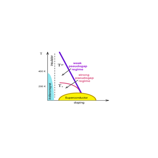
FIG. 1.: Schematic phase diagram of underdoped cuprates. Note the presence of two different crossover temperatures: $T^{\rm cr}$, which characterizes the onset of sizable antiferromagnetic correlations; and $T^{*}$, which signals the onset of a considerable loss of low energy spectral weight in the quasiparticle spectrum leading to a minimum of the characteristic spin-fluctuation energy $\omega_{\rm sf}$. The region between $T^{\rm cr}$ and $T^{*}$ is the weak pseudogap regime discussed in this paper.

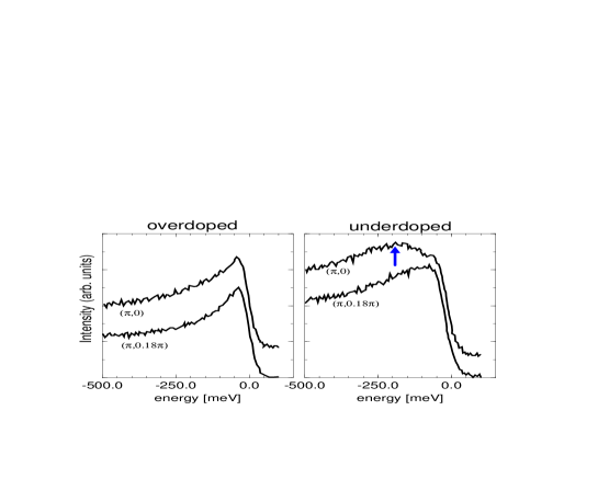
FIG. 2.: ARPES spectra from Ref.[30] for momenta ${\bf k}$ at and close to $(\pi,0)$, for two different doping concentrations.The $T_{\rm c}=78\,{\rm K}$ sample is slightly overdoped whereas the $T_{\rm c}=88\,{\rm K}$ sample is underdoped.

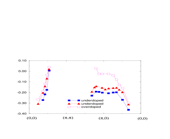
FIG. 3.: The position of local maxima of the spectral function along the high symmetry lines of the Brillouin zone is shown for an overdoped and underdoped system (data from Ref. [31]).

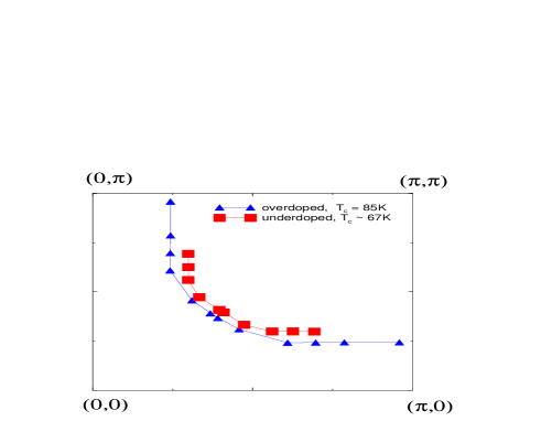
FIG. 4.: Fermi surface for an overdoped and underdoped system, obtained from ${\bf k}$-points where local maxima of the spectral function cross the Fermi energy (data from Ref. [31]).

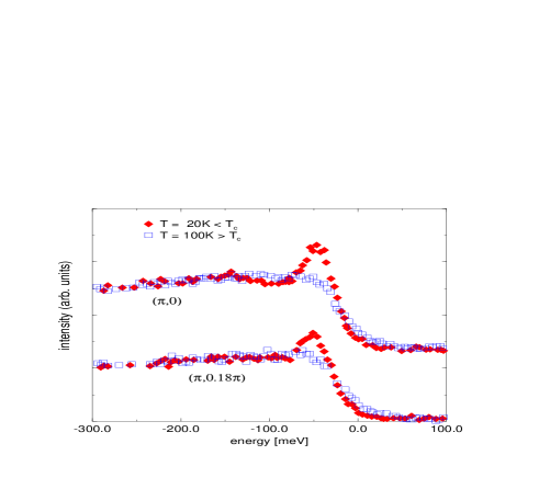
FIG. 5.: Spectral function of a hot quasiparticle above and below the superconducting transition temperature (data from Ref. [22]).

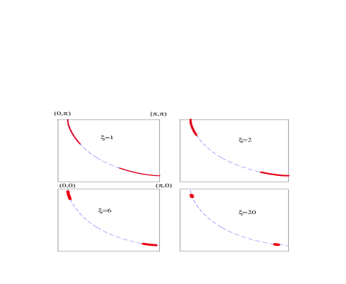
FIG. 6.: A typical bare Fermi surface in the first quarter of the BZ, closed around the momentum point $(\pi,\pi)$, for different AF correlation lengths. The thick sections characterize the hot parts of the Fermi surface.

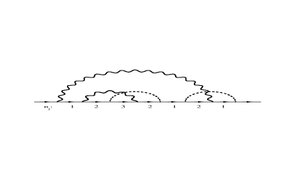
FIG. 7.: Illustration of the sequence $\{n_{j}\}$ for a self energy diagram of order $g^{8}$. $n_{j}$ is the number of spin fluctuation lines above the $j$-th fermionic Green’s function.

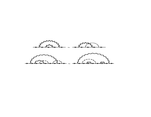
FIG. 8.: Self energy diagrams of order $g^{4}$ and $g^{8}$, which are, within the quasistatic approximation, identical apart from multiplicity and sign, because the number of spin fluctuation lines (shown by wiggly lines for transverse and dashed lines for longitudinal spin excitations) on top of a given electron propagator (solid line) are the same.

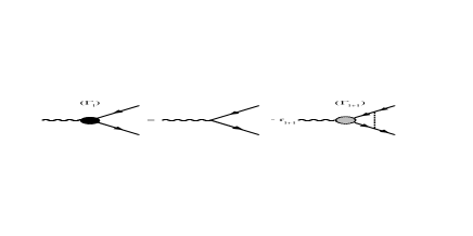
FIG. 9.: Diagrammatic illustration of the recursion relation of the vertex function, which is similar to the ladder approximation of the irreducible vertex. All non-ladder diagrams are taken into account by the corresponding weighting factors $r_{l+1}$.

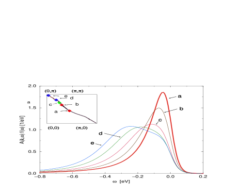
FIG. 10.: The spectral density multiplied with Fermi function on the Fermi surface for $\xi=3$.The distinct behavior of hot and cold quasiparticles is visible.

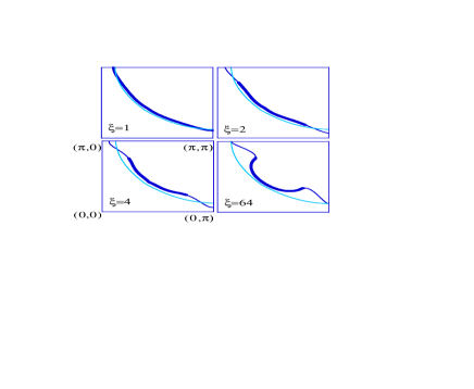
FIG. 11.: Fermi surface (solid line), in comparison with the bare Fermi surface (dotted line) and the visible part of the Fermi surface (thick solid line), i.e only for momenta where a maximum of the spectral density crosses the Fermi energy if ${\bf k}$ crosses the Fermi surface.

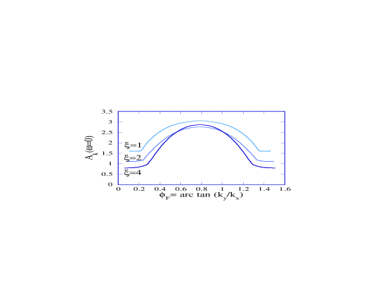
FIG. 12.: The spectral density $A_{\bf k}(\omega=0)$ along the Fermi surface as function of $\phi_{\rm F}={\rm arctan}(k_{y}/k_{x})$.

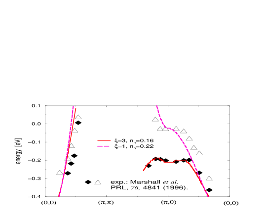
FIG. 13.: the momentum dependence of local maxima of the spectral density as function of $\xi$ and hole doping concentration $n_{h}$ is compared with the experiments of Ref. [25] for Bi₂Sr₂Ca_1-xDy_xCu₂O_8+δ with $x=0.1$ (triangles) and $x=0.175$ (diamonds). Only maxima with relative spectral weight $>10\%$ are shown.

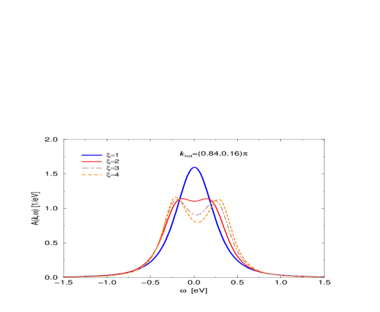
FIG. 14.: $\xi$ dependence of the spectral density at the hot spot. The appearance of SDW precursors for $\xi>2$ can be seen. For smaller values of $\xi$ the system behaves conventionally.

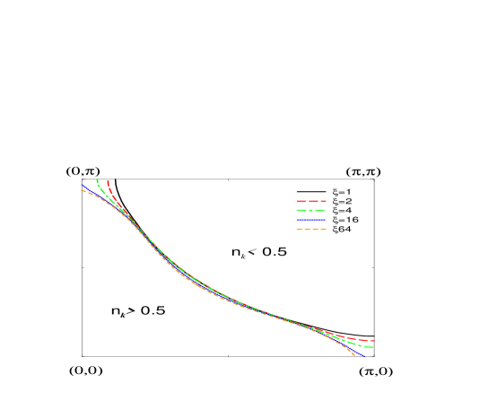
FIG. 15.: ${\bf k}$ -points with $n_{\bf k}=\frac{1}{2}$ for different correlation lengths in comparison with the results for an uncorrelated Fermi system.

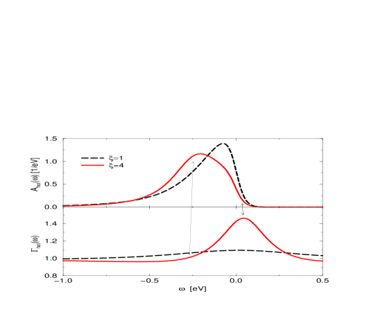
FIG. 16.: The spectral density $A_{\bf k}(\omega)$ and spin vertex function $\Gamma^{{\rm s}}_{{\bf k},{\bf k}+{\bf Q}}(\omega+i0^{+},\omega+i0^{+})$ for a hot quasiparticle with momentum transfer ${\bf Q}$ and zero frequency transfer as function of energy are shown for two correlation lengths.

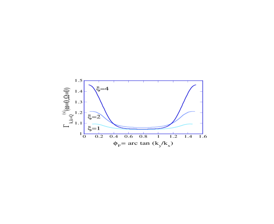
FIG. 17.: Spin vertex $\Gamma^{{\rm s}}_{{\bf k},{\bf k}+{\bf Q}}(\omega+i0^{+},\omega+i0^{+})$ for $\omega=0$ along the Fermi surface as function of $\phi_{\rm F}={\rm arctan}(k_{y}/k_{x})$.

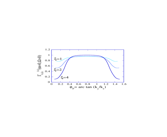
FIG. 18.: Charge vertex $\Gamma^{{\rm c}}_{{\bf k},{\bf k}+{\bf Q}}(\omega+i0^{+},\omega+i0^{+})$ for $\omega=0$ as a function of $\phi_{\rm F}={\rm arctan}(k_{y}/k_{x})$.

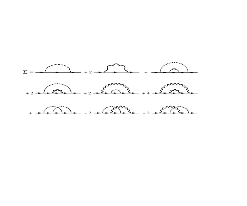
FIG. 19.: Self energy diagrams of the spin fermion model up to order $g^{4}$, including signs and multiplicities. The wiggly (dashed) lines correspond to spin flip (spin conserving) processes. Each crossing of a wiggly and dashed lines causes a prefactor $-1$ and each wiggly line an additional factor of $2$. The solid line corresponds to the bare fermion propagator and each vertex to the coupling constant $g/3^{1/2}$.

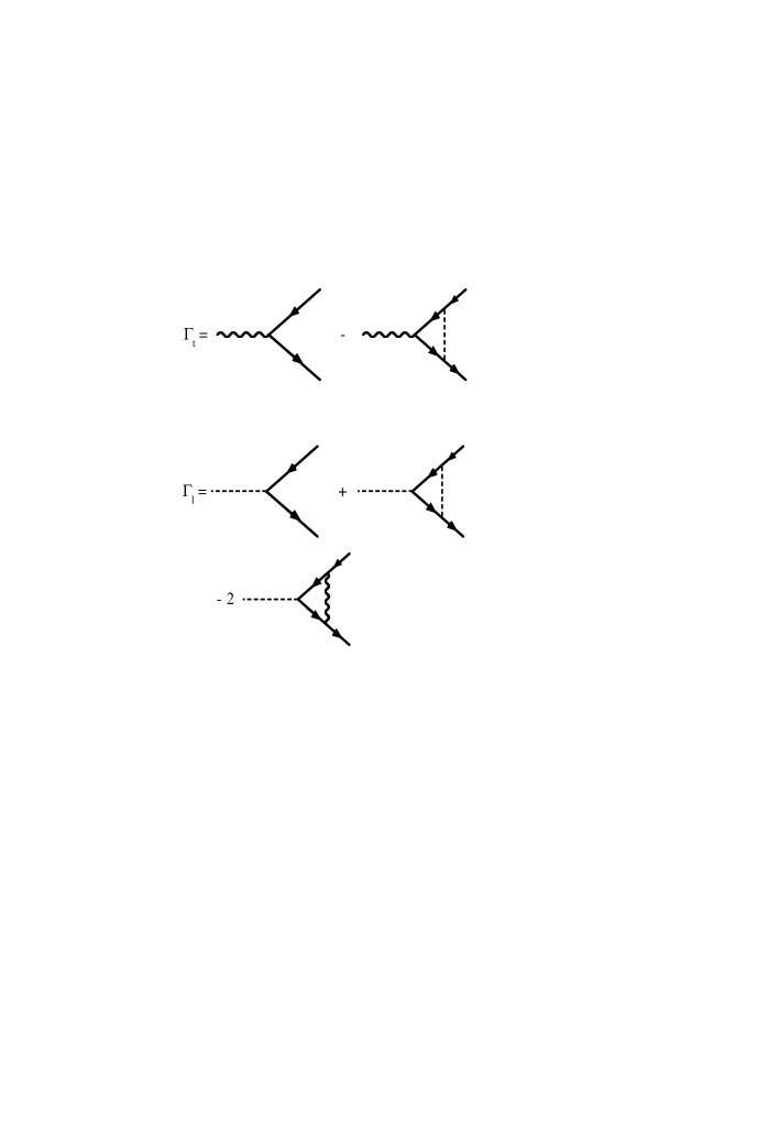
FIG. 20.: Longitudinal (spin conserving) and transverse (spin flip) vertices up to $g^{2}$. Note, that the derived diagrammatic rules guarantee, as expected, spin rotation invariance: $\Gamma_{\rm l}=\Gamma_{\rm t}$.

REFERENCES

- [1] D. Pines, Z. Phys. B103, 129 (1997); Proc. of the NATO ASI on The Gap Symmetry and Fluctuations in High Tc Superconductors, J. Bok and G. Deutscher, eds., Plenum Pub. (1998).
- [2] A.P. Kampf and J.R. Schrieffer, Phys. Rev. B 42, 7967 (1990).
- [3] E. Dagotto, A. Nazarenko and A. Moreo, Phys. Rev. Lett 74, 310 (1995).
- [4] A.V. Chubukov and D.K. Morr, Phys. Rep., 288, 355 (1997).
- [5] A. V. Chubukov, D. Pines, and B. P. Stojković, J. Phys.: Condens. Matter 8, 10017 (1996).
- [6] R. Preuss, W. Hanke, C. Gröber, and H. G. Evertz, Phys. Rev. Lett. 79 1122 (1997).
- [7] J. Schmalian, S. Grabowski, and K. H. Bennemann, Phys. Rev. B 56, R509 (1997).
- [8] V. Emery and S. A. Kivelson, Nature (London) 374, 434 (1995).
- [9] J. Maly, K. Levin, Phys. Rev. B 55, R15657 (1996); B. Janko, J. Maly, K. Levin, Phys. Rev. B 56, R11407 (1997).
- [10] J. Engelbrecht, M. Randeria, C. A. R. Sa de Melo, Phys Rev B 55, 15153 (1997).
- [11] V. Emery and S. A. Kivelson, Phys. Rev. Lett.74, 3253 (1995).
- [12] P. A. Lee and N. Nagaosa, Phys. Rev. B45, 966 (1992); ibid 46, 5621 (1992).
- [13] P. W. Anderson, The Theory of Superconductivity in the High-Tc Cuprate Superconductors (Princeton, Princeton, 1997).
- [14] H. Y. Hwang et al, Phys. Rev. Lett.72, 2636 (1994).
- [15] C. P. Slichter, in Strongly Correlated Electron Systems, ed. K. S. Bedell et al. (Addison-Wesley, Reading, MA,1994).
- [16] V. Barzykin and D. Pines, Phys. Rev. B 52, 13585 (1995).
- [17] H. Alloul, P. Mendels, G. Collin, and Ph. Monod, Physica C 156, 355 (1988).
- [18] J. Friedel, J. Phys. Condens. Matter 1, 7757 (1989).
- [19] N. J. Curro, T. Imai, C. P. Slichter, and B. Dabrowski, Phys. Rev. B 56, 877 (1997).
- [20] G. Aeppli, T. E. Mason, S. M. Hayden, H. A. Mook, J. Kulda, Science 278, 1432 (1997).
- [21] J. Schmalian, D. Pines, and B. Stojković, to appear in Phys. Rev. Lett. 80, No. 17 (1998).
- [22] A. G. Loeser, et al., Science, 273, 325 (1996).
- [23] H. Ding, et al., Nature, 382, 51 (1996).
- [24] C. Renner, O. Fischer to appear in Phys. Rev. Letters.
- [25] A. V. Puchkov, D. N. Basov, and T. Timusk, J. Phys. Condens. Matter 8, 10049 (1996), and references therein.
- [26] G. Blumberg, M. Kang, M. V. Klein, K. Kadowaki, C. Kendziora, Science 278, 1374 (1997).
- [27] R. Nemetschek, M. Opel, C. Hoffmann, P. Müller, R. Hackl, H. Berger, L. Forro, A. Erb, E. Walker, Phys. Rev. Lett. 78, 4837 (1997).
- [28] B. Bucher et al., Phys. Rev. Lett. 70, 2012 (1993).
- [29] M. V. Sadovskii, Sov. Phys. JETP 50, 989 (1979); J. Moscow Phys. Soc. 1, 391 (1991). see also R. H. McKenzie and D. Scarratt, Phys Rev. B 54, R12709 (1996).
- [30] P. J. White et al., Phys. Rev. B 54, 15669 (1996).
- [31] D. S. Marshall et al., Phys. Rev. Lett. 76, 4841 (1996).
- [32] P. Monthoux and D. Pines, Phys. Rev. B 47, 6069 (1993); ibid 48, 4261 (1994).
- [33] P. Monthoux, A. Balatsky, and D. Pines, Phys. Rev. Lett. 67, 3448 (1993); Phys. Rev. B 46, 14803 (1992).
- [34] D. Pines, P. Monthoux, J. Phys. Chem. Solids, 56, 1651 (1995).
- [35] A. Millis, H. Monien, and D. Pines, Phys. Rev. B 42, 1671 (1990).
- [36] Y. Zha, V. Barzykin, and D. Pines, Rev. B 54, 2561 (1996).
- [37] R. Hlubina and T.M. Rice, Phys. Rev. B 51, 9253 (1995); ibid 52, 13043 (1995).
- [38] B. P. Stojković and D. Pines, Phys. Rev. Lett. 76, 811 (1996); Phys. Rev. B 55, 8576 (1997).
- [39] Pengcheng Dai, H. A. Mook, and F. Dogan, Phys. Rev. Lett. 80, 1738, (1998).
- [40] F. C. Zhang and T. M. Rice, Phys. Rev. B37, 3759 (1988).
- [41] A. Chubukov, D. Morr, and K. A. Shakhnovich, Phil. Mag. B 74, 563 (1994).
- [42] P. V. Elyutin, Opt. Spektrosk. 43, 542 (1977); Opt. Spectrosc. (USSR) 43, 318 (1997).
- [43] O. Tchernyshyov, private communication.
- [44] Since the modified Bessel function of Eq. 23 diverges logarithmically for , care must be taken in the evaluation of . In fact, this divergence occurs only for infinite momentum cut off . Otherwise one finds , which can be absorbed into as in the case of the second order diagram.
- [45] J. R. Schrieffer, J. Low Temp. Phys. 99, 397 (1995).
- [46] A. V. Chubukov, preprint.
- [47] A. V. Chubukov and J. Schmalian, to appear as rapid communication in Phys. Rev. B, 01 May 98
- [48] P. Monthoux, Phys. Rev. B 55, 15261 (1997); A. V. Chubukov, P. Monthoux, and D. K. Morr, Phys. Rev. B 56, 7789 (1997).
- [49] Y. Ando, G. S. Boebinger, A. Passner, T. Kimura, K. Kishio, Phys. Rev. Lett. 75, 4662 (1995).
- [50] In this paper we ignore the role of incommensurations, which may even be adequate for the slight incommensurations found in YBCO, but which is problematic for La1.86Sr0.14CuO4. Considering the role of multiple scattering processes it follows that transitions such as are possible. Since in the commensurate case, is always a reciprocal lattice vector, . Therefore, incommensurate scattering reduces the decay probability of the states, causing the broadening of the high energy feature to be smaller. Note, a large incommensuration in this context means larger than twice the distance of the hot spot from .
- [51] A. J. Millis, Phys. Rev. B 48, 7183 (1993).
- [52] Although, Eq. B9 is valid only if and (I. S. Gradshteyn, I. M. Ryzhik; Table of integrals, Series, and Products, Academic Press, San Diego (1980)), the continued fraction representation is applicable for the more general case and . We proved this in a way similar to a method found in: N. M. Temme, Special Functions an Introduction to the Classical Functions of Mathematical Physics , Johm Wiley & Sons, New York, (1996).