The influence of magnetic-field-induced spin-density-wave motion and finite temperature on the quantum Hall effect in quasi-one-dimensional conductors: A quantum field theory

Abstract

We derive the effective action for a moving magnetic-field-induced spin-density wave (FISDW) in quasi-one-dimensional conductors at zero and nonzero temperatures by taking the functional integral over the electron field. The effective action consists of the (2+1)D Chern-Simons term and the (1+1)D chiral anomaly term, both written for a sum of the electromagnetic field and the chiral field associated with the FISDW phase. The calculated frequency dependence of Hall conductivity interpolates between the quantum Hall effect at low frequencies and zero Hall effect at high frequencies, where the counterflow of FISDW cancels the Hall current. The calculated temperature dependence of the Hall conductivity is interpreted within the two-fluid picture, by analogy with the BCS theory of superconductivity.

I INTRODUCTION

Organic metals of the (TMTSF)₂X family, where TMTSF is tetramethyltetraselenafulvalene and X represents an inorganic anion such as ClO₄ or PF₆, are highly anisotropic, quasi-one-dimensional (Q1D) crystals that consist of parallel conducting chains (see reviews [3, 4]). The electron wave functions overlap and the electric conductivity are the highest in the direction of the chains (the a direction) and are much smaller in the b direction perpendicular to the chains. In this paper, we neglect coupling between the chains in the third, c direction, which is weaker than in the b direction, and model (TMTSF)₂X as a system of uncoupled two-dimensional (2D) layers parallel to the a-b plane, each of the layers having a strong Q1D anisotropy. We choose the coordinate axis $x$ along the chains and the axis $y$ perpendicular to the chains within a layer.

A moderate magnetic field $H$ of the order of several Tesla, applied perpendicular to the layers, induces the so-called magnetic-field-induced spin-density wave (FISDW) in the system (see review [5]). In the FISDW state, the electron spin density is periodically modulated along the chains with the wave vector

$$Q_{x}=2k_{F}-NG,$$ (1)

where $k_{F}$ is the Fermi wave vector of the electrons, $N$ is an integer that characterizes FISDW, and

$$G=\frac{ebH}{\hbar c}$$ (2)

is a characteristic wave vector of the magnetic field. In Eq. (2), $e$ is the electron charge, $\hbar=h/2\pi$ is the Planck constant, $c$ is the speed of light, and $b$ is the distance between the chains. The longitudinal wave vector of FISDW (1) is not equal to $2k_{F}$ (as it would in a purely one-dimensional (1D) case), but deviates by an integer multiple of the magnetic wave vector $G$. When the magnetic field changes, the integer $N$ stays constant within a certain range of the magnetic field, then switches to another value, and so on. Thus, the system exhibits a cascade of the FISDW phase transitions when the magnetic field changes. The theory of FISDW was initiated by Gor’kov and Lebed’ [6], further developed in Refs. [7, 8, 9, 10, 11, 12, 13, 14, 15], and reviewed in Refs. [16, 17].

Within each FISDW phase, the Hall conductivity per one layer, $\sigma_{xy}$, has an integer quantized value at zero temperature:

$$\sigma_{xy}=\frac{2Ne^{2}}{h},$$ (3)

where $N$ is the same integer that appears in Eq. (1) and characterizes FISDW. (The factor 2 in Eq. (3) comes from the two orientations of the electron spin.) A gap in the energy spectrum of the electrons, which is a necessary condition for the quantum Hall effect (QHE), is supplied by FISDW. The theory of QHE in the FISDW state of Q1D conductors was developed in Refs. [18, 19, 20] (see also reviews [17, 21]). The theory assumes that FISDW is pinned and acts on electrons as a static periodic potential, so that Eq. (3) represents QHE [22] in a 2D periodic potential produced by FISDW and the chains.

On the other hand, under certain conditions, a density wave in a Q1D conductor can move (see, for example, reviews [23]). It is interesting to find out how this motion would affect QHE. Since the density-wave condensate can move only along the chains, at first sight, this purely 1D motion cannot contribute to the Hall effect, which is essentially a 2D effect. Nevertheless, we show in this paper that in the case of FISDW, unlike in the case of a regular charge- or spin-density wave (CDW/SDW), a nonstationary motion of the FISDW condensate does produce a nontrivial contribution to the Hall conductivity. In an ideal system, where FISDW is not pinned or damped, this additional contribution due to the FISDW motion (the so-called Fröhlich conductivity [23]) would exactly cancel the bare QHE, so that the resultant Hall conductivity would be zero. In real systems, this effect should result in vanishing of the ac Hall conductivity at high enough frequencies, where the dynamics of FISDW is dominated by inertia, and pinning and damping can be neglected. Because we study an interplay between QHE and the Fröhlich conductivity, our theory has some common ideas with the so-called topological superconductivity theory [24], which also seems to contain these ingredients. Frequency dependence of the Hall conductivity in a FISDW system was studied theoretically in Ref. [25]. However, because this theory fails to produce QHE at zero frequency, it is unsatisfactory. Some unsuccessful attempts to derive an effective action for a moving FISDW and QHE were made in Ref. [26].

Another interesting question is how the Hall conductivity in the FISDW state depends on temperature $T$. Our calculations show that thermal excitations across the FISDW energy gap partially destroy QHE, and $\sigma_{xy}(T)$ interpolates between the quantized value (3) at zero temperature and zero value at the transition temperature $T_{c}$, where FISDW disappears. We find that $\sigma_{xy}(T)$ has a temperature dependence similar to that of the superfluid density in the BCS theory of superconductivity. Thus, at a finite temperature, one might think of a two-fluid picture of QHE, where the Hall conductivity of the condensate is quantized, but the condensate fraction of the total electron density decreases with increasing temperature. An attempt to calculate the Hall conductivity in the FISDW state at a finite temperature was made in Ref. [25], but it failed to produce QHE at zero temperature.

Some of our results were briefly reported in conference proceedings [27]. They were also presented on a heuristic, semiphenomenological level in our review [21]. In the current paper, we present a systematic derivation of these results within the quantum-field-theory formalism. In Sec. II, we heuristically derive the effective Lagrangian of a moving FISDW and the corresponding ac Hall conductivity. In Sec. III, as a warmup exercise, we formally derive the effective action of a (1+1)D CDW/SDW in order to demonstrate that our method reproduces well-known results in this case. In the quantum-field theory, this effective action is usually associated with the so-called chiral anomaly [28, 29, 30]. Our method of derivation is close to that of Ref. [31]. In Sec. IV, we generalize the method of Sec. III to the case of (2+1)D FISDW and derive the effective action for a moving FISDW. We find that, in addition to the (1+1)D chiral anomaly term, the effective action contains the (2+1)D Chern-Simons term, written for a combination of electromagnetic potentials and gradients of the FISDW phase. This modified Chern-Simons term describes both the QHE of a static FISDW and the effect of FISDW motion. The results are consistent with the heuristic derivation of Sec. II. In Sec. V, we rederive the results of Sec. IV using an alternative method, which then is straightforwardly generalized to a finite temperature in Sec. VI. The results for a finite temperature are obtained heuristically in Sec. VI A and formally in Sec. VI B. Experimental implications of our theory are discussed in Sec. VII. Conclusions are given in Sec. VIII.

II SEMIPHENOMENOLOGICAL APPROACH TO QHE AND MOTION OF FISDW

A Fröhlich current and Hall current

We consider a 2D system where electrons are confined to the chains parallel to the $x$ axis, and the spacing between the chains along the $y$ axis is equal to $b$. A magnetic field $H$ is applied along the $z$ axis perpendicular to the $(x,y)$ plane. The system is in the FISDW state at zero temperature. In order to calculate the Hall effect, let us apply an electric field ${\cal E}_{y}$ perpendicular to the chains. The electron Hamiltonian ${\mathbb{H}}$ can be written as

$${\mathbb{H}} = -\frac{\hbar^{2}}{2m}\frac{\partial^{2}}{\partial x^{2}}+2\Delta\cos(Q_{x}x+\Theta)$$ (5)

$$+2t_{b}\cos(k_{y}b-Gx+\Omega_{y}t),$$

where $k_{y}$ is the electron wave vector perpendicular to the chains. In the r.h.s. of Eq. (5), the first term represents the kinetic energy of the electron motion along the chains with the effective mass $m$. The second term describes the periodic potential produced by FISDW. The FISDW potential is characterized by the longitudinal wave vector $Q_{x}$ (1), an amplitude $\Delta$, and a phase $\Theta$. The third term describes the electron tunneling between the nearest neighboring chain with the amplitude $t_{b}$. In the gauge $A_{y}=Hx-c{\cal E}_{y}t$ and $\phi=A_{x}=A_{z}=0$, the magnetic and the transverse electric fields appear in the third term of Hamiltonian (5) via the Peierls-Onsager substitution $k_{y}\rightarrow k_{y}-eA_{y}/c\hbar$, where $\Omega_{y}=eb{\cal E}_{y}/\hbar$, and $G$ is given by Eq. (2). Strictly speaking, a complete theory of FISDW requires us to take into account the transverse component $Q_{y}$ of the FISDW wave vector and the electron tunneling between the next-nearest neighboring chains with the amplitude $t_{b}^{\prime}$ [8, 9, 10, 11]. However, while $t_{b}^{\prime}$ and $Q_{y}$ are very important for determining the properties of FISDW, such as $N$, $\Delta$, and $T_{c}$, $t_{b}^{\prime}$ and $Q_{y}$ are not essential for the theory of QHE, so we set them at zero in order to simplify presentation. We do not pay attention to the spin structure of the density-wave order parameter in Eq. (5), because it is immaterial for our study, which focuses on the orbital effect of the magnetic field. To simplify the presentation, we study the case of CDW, but the results for SDW are the same.

In the presence of the magnetic field $H$, the interchain hopping term in Eq. (5) acts as a potential, periodic along the chains with the wave vector $G$ proportional to $H$. In the presence of the transverse electric field ${\cal E}_{y}$, this potential moves along the chains with the velocity $\Omega_{y}/G=c{\cal E}_{y}/H$ proportional to ${\cal E}_{y}$. This velocity is nothing but the drift velocity in crossed electric and magnetic fields. The FISDW potential may also move along the chains, in which case its phase $\Theta$ depends on time $t$, and the velocity of the motion is proportional to the time derivative $\dot{\Theta}$. We are interested in a spatially homogeneous motion of FISDW, so let us assume that $\Theta$ depends only on time $t$ and not on the coordinates $x$ and $y$. We also assume that both potentials move very slowly, adiabatically, which is the case when the electric field is sufficiently weak.

Let us calculate the current along the chains produced by the motion of the potentials. Since there is an energy gap at the Fermi level, following the arguments of Laughlin [32] we can say that an integer number of electrons $N_{1}$ is transferred from one end of a chain to another when the FISDW potential shifts by its period $l_{1}=2\pi/Q_{x}$. The same is true for the motion of the interchain hopping potential with an integer $N_{2}$ and the period $l_{2}=2\pi/G$. Suppose that the first potential shifts by an infinitesimal displacement $dx_{1}$ and the second by $dx_{2}$. The total transferred charge $dq$ would be the sum of the prorated amounts of $N_{1}$ and $N_{2}$:

$$dq=eN_{1}\frac{dx_{1}}{l_{1}}+eN_{2}\frac{dx_{2}}{l_{2}}.$$ (6)

Now, suppose that both potentials are shifted by the same displacement $dx=dx_{1}=dx_{2}$. This corresponds to a translation of the system as a whole, so we can write that

$$dq=e\rho\,dx,$$ (7)

where $\rho=4k_{F}/2\pi$ is the concentration of electrons. Equating (6) and (7) and substituting the expressions for $\rho$, $l_{1}$, and $l_{2}$, we find the following Diophantine-type equation [33]:

$$4k_{F}=N_{1}(2k_{F}-NG)+N_{2}G.$$ (8)

Since $k_{F}/G$ is, in general, an irrational number, the only solution of Eq. (8) for the integers $N_{1}$ and $N_{2}$ is $N_{1}=2$ and $N_{2}=N_{1}N=2N$.

Dividing Eq. (6) by a time increment $dt$ and the interchain distance $b$, we find the density of current along the chains, $j_{x}$. Taking into account that according to Eq. (5) the displacements of the potentials are related to their phases: $dx_{1}=-d\Theta/Q_{x}$ and $dx_{2}=\Omega_{y}dt/G$, we find the final expression for $j_{x}$:

$$j_{x}=-\frac{e}{\pi b}\dot{\Theta}+\frac{2Ne^{2}}{h}{\cal E}_{y}.$$ (9)

The first term in Eq. (9) represents the contribution of the FISDW motion, the so-called Fröhlich conductivity [23]. This term vanishes when the FISDW is pinned and does not move ($\dot{\Theta}=0$). The second term in Eq. (9) describes QHE, in agreement with Eq. (3).

B Effective Lagrangian

To complete the solution of the problem, it is necessary to find how $\dot{\Theta}$ depends on ${\cal E}_{y}$. For this purpose, we need the equation of motion for $\Theta$, which can be derived once we know the Lagrangian density of the system, $L$. Two terms in $L$ can be readily recovered taking into account that the current density $j_{x}$, given by Eq. (9), is the variational derivative of the Lagrangian density with respect to the electromagnetic vector potential $A_{x}$: $j_{x}=c\,\delta L/\delta A_{x}$. Written in a gauge-invariant form, the recovered part of the Lagrangian density is equal to

$$L_{1}=\frac{Ne^{2}}{2\pi\hbar c}\varepsilon_{ijk}A^{i}\frac{\partial A^{k}}{\partial x_{j}}-\frac{e}{\pi b}\Theta{\cal E}_{x},$$ (10)

where the first term is the so-called Chern-Simons term responsible for QHE [19], and the second term describes the interaction of the density-wave condensate with the electric field along the chains ${\cal E}_{x}=-\partial A_{x}/c\partial t-\partial\phi/\partial x$ [23]. In Eq. (10), we use the relativistic notation [34] with the indices $(i,j,k)$ taking the values $(0,1,2)$ and the implied summation over repeated indices [35]. The contravariant vectors have the superscript indices: $A^{i}=(\phi,A_{x},A_{y})$ and $x^{j}=(ct,x,y)$. The covariant vectors have subscript indices: $x_{j}=(ct,-x,-y)$, and are obtained from the contravariant vectors by applying the metric tensor of the Minkowski space: $g_{ij}=g^{ij}={\rm diag}(1,-1,-1)$. $\varepsilon_{ijk}$ is the antisymmetric tensor with $\varepsilon_{012}=1$. The potentials $A^{i}$ and the corresponding fields ${\cal E}_{x}$, ${\cal E}_{y}$, and ${\cal H}_{z}$ represent an infinitesimal external electromagnetic field. These potentials do not include the vector potential of the bare magnetic field $H$, which is incorporated into the Hamiltonian of the system via the term $Gx$ in Eq. (5) with $G$ given by Eq. (2).

Lagrangian density (10) should be supplemented with the kinetic energy of the FISDW condensate, $K$. The FISDW potential itself has no inertia, because it is produced by the instantaneous Coulomb interaction between electrons, so $K$ originates completely from the kinetic energy of the electrons confined under the FISDW energy gap. Thus $K$ is proportional to the square of the average electron velocity, which, in turn, is proportional to the electric current along the chains:

$$K=\frac{\pi\hbar b}{4v_{F}e^{2}}\,j_{x}^{2},$$ (11)

where $v_{F}=\hbar k_{F}/m$ is the Fermi velocity. Substituting Eq. (9) into Eq. (11), expanding, and omitting an unimportant term proportional to ${\cal E}_{y}^{2}$, we obtain the second part of the Lagrangian density of the system:

$$L_{2}=\frac{\hbar}{4\pi bv_{F}}\dot{\Theta}^{2}-\frac{eN}{2\pi v_{F}}\dot{\Theta}{\cal E}_{y}.$$ (12)

The first term in Eq. (12) is the same as the kinetic energy of a purely 1D density wave [23] and is not specific to FISDW. The most important is the second term, which describes the interaction of the FISDW motion and the electric field perpendicular to the chains. This term is allowed by symmetry in the considered system and has the structure of a mixed vector–scalar product:

$${\bf v}[\mbox{\boldmath${\cal E}$}\times{\bf H}].$$ (13)

Here, ${\bf v}$ is the velocity of the FISDW, which is proportional to $\dot{\Theta}$ and is directed along the chains, that is, along the $x$ axis. The magnetic field H is directed along the $z$ axis, thus allowing the electric field ${\cal E}$ to enter only through the component ${\cal E}_{y}$. Comparing Eq. (13) with the last term in Eq. (12), one should take into account that the magnetic field enters the last term implicitly, through the integer $N$, which depends on $H$ and changes sign when $H$ changes sign.

Varying the total Lagrangian $L=L_{1}+L_{2}$, given by Eqs. (10) and (12), with respect to $A_{y}$, we find the current density across the chains:

$$j_{y}=-\frac{2Ne^{2}}{h}{\cal E}_{x}-\frac{eN}{2\pi v_{F}}\ddot{\Theta}.$$ (14)

In the r.h.s. of Eq. (14), the first term describes the quantum Hall current, whereas the second term, proportional to the acceleration of the FISDW condensate, comes from the second term in Eq. (12) and reflects the contribution of the FISDW motion along the chains to the electric current across the chains.

Setting the variational derivative of $L$ with respect to $\Theta$ to zero, we find the equation of motion for $\Theta$:

$$\ddot{\Theta}=-\frac{2ev_{F}}{\hbar}{\cal E}_{x}+\frac{eNb}{\hbar}\dot{\cal E}_{y}.$$ (15)

In Eq. (15), the first two terms constitute the standard 1D equation of motion of the density wave[23], whereas the last term, proportional to the time derivative of ${\cal E}_{y}$, which originated from the last term in Eq. (12), describes the influence of the electric field across the chains on the motion of FISDW.

C Hall conductivity

In order to see the influence of the FISDW motion on the Hall effect, let us consider the two cases, where the electric field is applied either perpendicular or parallel to the chains. In the first case, ${\cal E}_{x}=0$, so integrating Eq. (15) in time, we find that $\dot{\Theta}=eNb{\cal E}_{y}/\hbar$. Substituting this equation into Eq. (9), we see that the first term (the Fröhlich conductivity of FISDW) precisely cancels the second term (the quantum Hall current), so the resulting Hall current is equal to zero. This result could have been obtained without calculations by taking into account that the time dependence $\Theta(t)$ is determined by the principle of minimal action. The relevant part of the action is given, in this case, by Eq. (11), which attains the minimal value at zero current: $j_{x}=0$. We can say that if FISDW is free to move it adjusts its velocity to compensate the external electric field ${\cal E}_{y}$ and to keep zero Hall current. In the second case, where the electric field ${\cal E}_{x}$ is directed along the chains, it accelerates the density wave according to the equation of motion (15): $\ddot{\Theta}=-2ev_{F}{\cal E}_{x}/\hbar$. Substituting this equation into Eq. (14), we find again that the Hall current vanishes.

It is clear, however, that in stationary, dc measurements, the acceleration of the FISDW, discussed in the previous paragraph, cannot last forever. Any friction or dissipation will inevitably stabilize the motion of the density wave to a steady flow with zero acceleration. In this steady state, the second term in Eq. (14) vanishes, and the current $j_{y}$ recovers its quantum Hall value. The same is true in the case where the electric field is perpendicular to the chains. In that case, dissipation eventually stops the FISDW motion along the chains and restores $j_{x}$, given by Eq. (9), to the quantum Hall value. The conclusion is that the contribution of the moving FISDW condensate to the Hall conductivity is essentially nonstationary and cannot be observed in dc measurements.

On the other hand, the effect can be seen in ac experiments. To be realistic, let us add damping and pinning [23] to the equation of motion of FISDW (15):

$$\ddot{\Theta}+\frac{1}{\tau}\dot{\Theta}+\omega_{0}^{2}\Theta=-\frac{2ev_{F}}{\hbar}{\cal E}_{x}+\frac{eNb}{\hbar}\dot{\cal E}_{y},$$ (16)

where $\tau$ is the relaxation time and $\omega_{0}$ is the pinning frequency. Solving Eq. (16) via the Fourier transformation from the time $t$ to the frequency $\omega$ and substituting the result into Eqs. (9) and (14), we find the Hall conductivity as a function of frequency:

$$\sigma_{xy}(\omega)=\frac{2Ne^{2}}{h}\frac{\omega_{0}^{2}-i\omega/\tau}{\omega_{0}^{2}-\omega^{2}-i\omega/\tau}.$$ (17)

The absolute value of the Hall conductivity, $|\sigma_{xy}|$, computed from Eq. (17) is plotted in Fig. 1 as a function of $\omega/\omega_{0}$ for $\omega_{0}\tau=2$. As we can see in the figure, the Hall conductivity is quantized at zero frequency and has a resonance at the pinning frequency. At the higher frequencies, where pinning and damping can be neglected and the system effectively behaves as an ideal, purely inertial system considered in this section, the Hall conductivity does decrease toward zero.

FIG. 1.: Absolute value of the Hall conductivity in the FISDW state as a function of the frequency $\omega$ normalized to the pinning frequency $\omega_{0}$, as given by Eq. (17) with $\omega_{0}\tau=2$.

In this section, the derivation of results was heuristic. In the following sections, we calculate the effective action of a moving FISDW systematically, within the functional-integral formalism.

III EFFECTIVE ACTION FOR A (1+1)D DENSITY WAVE

As a warmup exercise, let us derive the effective action for a regular CDW/SDW in the (1+1)D case, where 1+1 represents the space coordinate $x$ and the time coordinate $t$. For simplicity, we consider the case of CDW; results for SDW are the same. Summation over the spin indices of electrons is assumed everywhere, which generates a factor of 2 in traces over the fermions.

Let us consider (1+1)D fermions, described by a Grassmann field $\Psi(t,x)$, in the presence a density-wave potential $2\Delta\cos[2k_{F}x+\Theta(t,x)]$ and an infinitesimal external electromagnetic field, described by the scalar $\phi(t,x)$ and vector $A_{x}(t,x)$ potentials. The action of the system is

$$S[\Psi,\Theta,\phi,A_{x}]=\int dt\,dx\,\Psi^{+}\biggl{[}\left(i\hbar\frac{\partial}{\partial t}-e\phi\right)$$ (18)

$${}-\frac{1}{2m}\left(-i\hbar\frac{\partial}{\partial x}-\frac{e}{c}A_{x}\right)^{2}+\varepsilon_{F}-2\Delta\cos(2k_{F}x+\Theta)\biggr{]}\Psi.$$ (19)

Let us introduce the doublet of fermion fields

$$\psi(t,x)={\psi_{+}(t,x)\choose\psi_{-}(t,x)}$$ (20)

with the momenta close to $\pm k_{F}$:

$$\Psi(t,x)=\psi_{+}(t,x)e^{ik_{F}x}+\psi_{-}(t,x)e^{-ik_{F}x}.$$ (21)

Substituting Eq. (21) into Eq. (18) and neglecting the terms with the higher derivatives $\partial^{2}\psi_{\pm}/\partial x^{2}$ and the terms where the fast-oscillating factors $\exp(\pm i2k_{F}x)$ do not cancel out, we rewrite the action of the system in the matrix form

$$S[\psi,\Theta,\phi,A_{x}]={\rm Tr}\int dt\,dx\,\psi^{+}{\cal L}[\Theta,\phi,A_{x}]\psi$$ (22)

with

$${\cal L}[\Theta,\phi,A_{x}]=\tau_{0}\left(i\hbar\frac{\partial}{\partial t}-e\phi\right)$$ (23)

$${}+\tau_{z}v_{F}\left(i\hbar\frac{\partial}{\partial x}+\frac{e}{c}A_{x}\right)-\tau_{x}\Delta e^{-i\tau_{z}\Theta}-\tau_{0}\frac{e^{2}}{2mc^{2}}A_{x}^{2}.$$ (24)

In Eq. (23), $\tau_{x}$, $\tau_{y}$, $\tau_{z}$, and $\tau_{0}$ are the $2\times 2$ Pauli matrices and the unit matrix acting on the doublet of fermion fields (20). In Eq. (22), the trace (Tr) is taken over the $\pm$ components of the fermion field (20) and the implied spin indices of the fermions.

It is convenient to rewrite Eq. (23) in a pseudorelativistic notation:

$${\cal L}[\Theta,A^{\mu}]=i\hbar v_{F}\tau_{\mu}\frac{\partial}{\partial x_{\mu}}-e\frac{v_{F}}{c}\tau_{\mu}A^{\mu}$$ (25)

$$-\tau_{x}\Delta e^{-i\tau_{z}\Theta}-\tau_{0}\frac{e^{2}}{2mc^{2}}A_{x}^{2},$$ (26)

where the index $\mu$ takes the values 0 and 1, and summation over repeated indices is implied. The contravariant vectors are defined as follows:

$$x^{\mu}=(v_{F}t,x),\;A^{\mu}=\left(\frac{c}{v_{F}}\phi,A_{x}\right),\;\tau^{\mu}=(\tau_{0},\tau_{z}).$$ (27)

The covariant vectors are obtained by applying the metric tensor: $g_{\mu\nu}=g^{\mu\nu}={\rm diag}(1,-1)$.

We wish to find the effective action of the system, ${\mathbb{S}}[\Theta,A^{\mu}]$, by carrying out the functional integral over the fermion fields $\psi$ in the partition function with the action $S[\psi,\Theta,A^{\mu}]$:

$$e^{i{\mathbb{S}}[\Theta,A^{\mu}]/\hbar}=\frac{\int{\cal D}\psi^{+}\,{\cal D}\psi\,e^{iS[\psi,\Theta,A^{\mu}]/\hbar}}{\int{\cal D}\psi^{+}\,{\cal D}\psi\,e^{iS[\psi,0,0]/\hbar}}.$$ (28)

The functional integral (28) with action (22) is difficult to treat, because the phase $\Theta(x^{\mu})$ in Eq. (23) is space-time dependent. In order to eliminate this problem, let us change the integration variable $\psi$ to a new variable $\tilde{\psi}$ via a chiral transformation characterized by a unitary matrix $U[\Theta(x^{\mu})]$ [36]:

$$\psi(x^{\mu})=U[\Theta(x^{\mu})]\,\tilde{\psi}(x^{\mu})=e^{i\tau_{z}\Theta(x^{\mu})/2}\,\tilde{\psi}(x^{\mu}).$$ (29)

Written in terms of the new field $\tilde{\psi}$, action (22) becomes

$$\tilde{S}[\tilde{\psi},\Theta,A^{\mu}]={\rm Tr}\int dt\,dx\,\tilde{\psi}^{+}\tilde{\cal L}\tilde{\psi},$$ (30)

where

$$\tilde{\cal L} = {\cal L}_{0}+{\cal L}_{1}+{\cal L}_{2},$$ (31)

$${\cal L}_{0} = i\hbar v_{F}\tau_{\mu}\frac{\partial}{\partial x_{\mu}}-\tau_{x}\Delta,$$ (32)

$${\cal L}_{1} = -e\frac{v_{F}}{c}\tau_{\mu}B^{\mu},$$ (33)

$${\cal L}_{2} = -\tau_{0}\frac{e^{2}}{2mc^{2}}A_{x}^{2}.$$ (34)

In Eq. (33),

$$B^{\mu} = A^{\mu}+a^{\mu},$$ (35)

$$a^{\mu} = \frac{\hbar c}{2e}\varepsilon^{\mu\nu}\frac{\partial\Theta}{\partial x^{\nu}},$$ (36)

where $\varepsilon^{\mu\nu}$ is the antisymmetric tensor with $\varepsilon^{01}=1$. The chiral transformation (29) eliminates the phase factor $\exp({-i\tau_{z}\Theta})$ of the order parameter $\Delta$ from Eq. (23), so that Lagrangian (32) acquires a simple form. As a tradeoff, Lagrangian (33) subjects fermions to the effective potential $B^{\mu}=A^{\mu}+a^{\mu}$ (35), which combines the original electromagnetic potentials $A^{\mu}$ and the gradients of the phase $\Theta$ (36):

$$a^{0}=\frac{\hbar c}{2e}\frac{\partial\Theta}{\partial x},\qquad a^{1}=-\frac{\hbar c}{2ev_{F}}\frac{\partial\Theta}{\partial t}.$$ (37)

Because the external electromagnetic potentials $A^{\mu}$ and the gradients of $\Theta$ are assumed to be small, the effective potentials $B^{\mu}$ are also small and can be treated perturbatively. Changing $\psi$ to $\tilde{\psi}$ and $S$ to $\tilde{S}$ in Eq. (28), we can calculate the effective action ${\mathbb{S}}[\Theta,A^{\mu}]$ by making a diagrammatic expansion in powers of $B^{\mu}$. Expanding to the first power of Lagrangian (33) and averaging over the fermions, we obtain the contribution ${\mathbb{S}}_{1}$ that is nominally of the first order in $B^{\mu}$. Expansion to the second power of (33) and the first power of (34) gives us the contributions ${\mathbb{S}}_{2}^{\prime}$ and ${\mathbb{S}}_{2}^{\prime\prime}$ of the second order in $B^{\mu}$ and $A_{x}$. First we calculate ${\mathbb{S}}_{2}={\mathbb{S}}_{2}^{\prime}+{\mathbb{S}}_{2}^{\prime\prime}$ in Sec. III A and then obtain ${\mathbb{S}}_{1}$ in Sec. III B.

A The second-order terms of the effective action

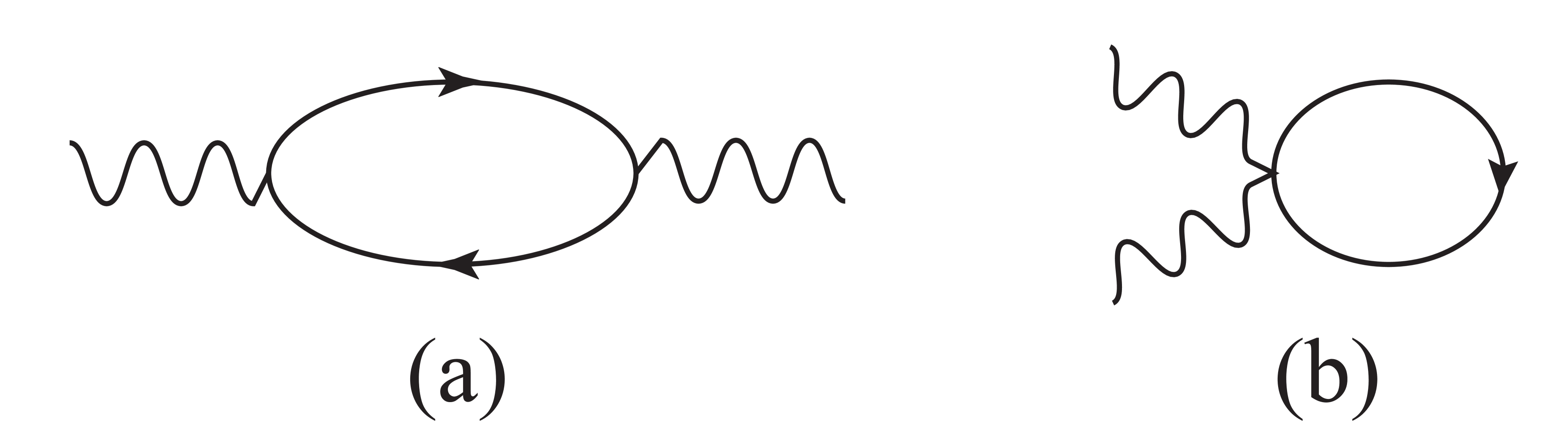
FIG. 2.: Two Feynman diagrams determining the second-order contribution to the effective action, ${\mathbb{S}}_{2}$. The solid lines represent the fermion Green functions (40). The wavy lines in panel (a) represent the effective potentials $B^{\mu}$ (35), which interact with the fermions via Eq. (33). The wavy lines in panel (b) represent the electromagnetic potential $A_{x}$, which interacts with the fermions via Eq. (34)

The two second-order contributions to the effective action, ${\mathbb{S}}_{2}^{\prime}$ and ${\mathbb{S}}_{2}^{\prime\prime}$, are given by the two Feynman diagrams shown in Fig. 2, where the wavy lines represent $B^{\mu}$ and the solid lines represent the bare Green functions ${\cal G}$ of the fermions:

$${\cal G}(t-t^{\prime},x-x^{\prime})=-\frac{i}{\hbar}\langle\psi(t,x)\psi^{+}(x^{\prime},t^{\prime})\rangle_{\tilde{S}_{0}}$$ (38)

$$=\int\frac{dk\,d\omega}{(2\pi)^{2}}e^{ik(x-x^{\prime})-i\omega(t-t^{\prime})}{\cal G}(k,\omega).$$ (39)

The Green function (39) is obtained by averaging the fermion fields using action $\tilde{S}_{0}$ (30) with the Lagrangian ${\cal L}_{0}$ (32):

$${\cal G}(k,\omega) = \frac{e^{i\epsilon\omega}}{\tau_{0}\hbar\omega-\tau_{z}v_{F}\hbar k-\tau_{x}\Delta+i\tau_{0}\epsilon\,{\rm sgn}(\omega)},$$ (40)

where $\epsilon>0$ is infinitesimal. Because $\psi$ and $\psi^{+}$ in Eq. (39) are two-component fields (20), the Green function ${\cal G}$ is a $2\times 2$ matrix. The factor $e^{i\epsilon\omega}$ in Eq. (40) ensures that the integral in $\omega$ of the Green function (40),

$$\int\frac{d\omega}{2\pi}{\rm Tr}[\tau_{z}{\cal G}(k,\omega)]=\frac{2i}{\hbar}\,[n_{+}(k)-n_{-}(k)],$$ (41)

gives the difference in the occupation numbers $n_{+}(k)$ and $n_{-}(k)$ of the $\pm$ fermions. The fermion occupation number $n$ is equal to 1 and 0 at the energies deeply below and high above the Fermi energy, correspondingly. This statement applies to the electron energies much greater than the energy gap $\Delta$. The factor 2 in Eq. (41) comes from the two orientations of the electron spin.

Introducing the Fourier transforms of the potentials

$$B_{\mu}(k,\omega)=\int dt\,dx\,e^{-ikx+i\omega t}B_{\mu}(t,x),$$ (42)

we find an analytical expression for the diagram shown in Fig. 2(a)

$${\mathbb{S}}_{2}^{\prime}=\frac{e^{2}v_{F}^{2}}{c^{2}}\int\frac{dp\,d\Omega}{(2\pi)^{2}}P^{\mu\nu}(p,\Omega)B_{\mu}(p,\Omega)B_{\nu}(-p,-\Omega),$$ (43)

where

$$P^{\mu\nu}(p,\Omega)=\frac{i\hbar}{2}\int\frac{dk\,d\omega}{(2\pi)^{2}}{\rm Tr}[\tau^{\mu}{\cal G}(k,\omega)\tau^{\nu}{\cal G}(k+p,\omega+\Omega)].$$ (44)

Assuming that the gradients of $B_{\mu}$ are small, we expand $P^{\mu\nu}(p,\Omega)$ in powers of $p$ and $\Omega$ and keep only the zeroth-order term, effectively setting $p=\Omega=0$ in Eq. (44). Thus, we need to calculate the following three integrals:

$$P^{00}(0,0)=\frac{i\hbar}{2}\int\frac{dk\,d\omega}{(2\pi)^{2}}{\rm Tr}[\tau_{0}{\cal G}(k,\omega)\tau_{0}{\cal G}(k,\omega)],$$ (45)

$$P^{11}(0,0)=\frac{i\hbar}{2}\int\frac{dk\,d\omega}{(2\pi)^{2}}{\rm Tr}[\tau_{z}{\cal G}(k,\omega)\tau_{z}{\cal G}(k,\omega)],$$ (46)

$$P^{10}(0,0)=\frac{i\hbar}{2}\int\frac{dk\,d\omega}{(2\pi)^{2}}{\rm Tr}[\tau_{z}{\cal G}(k,\omega)\tau_{0}{\cal G}(k,\omega)].$$ (47)

Using Eq. (40) and the identity

$$\partial{\cal G}=-{\cal G}(\partial{\cal G}^{-1}){\cal G},$$ (48)

where $\partial$ represent a derivative of ${\cal G}$ with respect to any parameter that ${\cal G}$ depends upon, we can rewrite Eqs. (45)–(47) in the following form:

$$P^{00(10)} = -\frac{i}{2}\int\frac{dk\,d\omega}{(2\pi)^{2}}\,{\rm Tr}\left(\tau_{0(z)}\frac{\partial{\cal G}(k,\omega)}{\partial\omega}\right),$$ (49)

$$P^{11} = \frac{i}{2v_{F}}\int\frac{dk\,d\omega}{(2\pi)^{2}}\,{\rm Tr}\left(\tau_{z}\frac{\partial{\cal G}(k,\omega)}{\partial k}\right).$$ (50)

In condensed matter physics, we integrate over the frequency $\omega$ first and than integrate over the wave vector $k$. Taking the integral over $\omega$ in Eq. (49), we find that, being an integral of a full derivative of ${\cal G}(k,\omega)$ with respect to $\omega$, the integral vanishes, because ${\cal G}(k,\pm\infty)$ vanishes:

$$P^{00}=P^{10}=0.$$ (51)

On the other hand, according to Eq. (41), the integral over $\omega$ in Eq. (50) gives

$$P^{11}=-\frac{1}{2\pi\hbar v_{F}}\int dk\,\frac{\partial[n_{+}(k)-n_{-}(k)]}{\partial k}=\frac{1}{\pi\hbar v_{F}}.$$ (52)

We took into account in Eq. (52) that the fermion occupation number $n$ is equal to 1 and 0 at the energies deeply below and high above the Fermi energy, correspondingly.

Substituting Eqs. (51) and (52) into Eq. (43), we find

$${\mathbb{S}}_{2}^{\prime} = \frac{e^{2}v_{F}}{\pi\hbar c^{2}}\int dt\,dx\,(B^{1})^{2}$$ (53)

$$= \frac{e^{2}v_{F}}{\pi\hbar c^{2}}\int dt\,dx\,\left(A_{x}-\frac{\hbar c}{2ev_{F}}\frac{\partial\Theta}{\partial t}\right)^{2}.$$ (54)

The analytical expression for the diagram shown in Fig. 2(b) is

$${\mathbb{S}}_{2}^{\prime\prime}=-\frac{e^{2}}{2mc^{2}}\int dt\,dx\,A_{x}^{2}\,{\rm Tr}\langle\psi^{+}(t,x)\tau_{0}\psi(t,x)\rangle_{\tilde{S}_{0}}.$$ (55)

Taking into account that the last factor in Eq. (55) is nothing but the average electron density $\rho=4k_{F}/2\pi$, we find

$${\mathbb{S}}_{2}^{\prime\prime}=-\frac{e^{2}v_{F}}{\pi\hbar c^{2}}\int dt\,dx\,A_{x}^{2}.$$ (56)

Combining Eqs. (54) and (56), we find the total second-order part of the effective action, ${\mathbb{S}}_{2}={\mathbb{S}}_{2}^{\prime}+{\mathbb{S}}_{2}^{\prime\prime}$:

$${\mathbb{S}}_{2}[\Theta,A^{\mu}]=\frac{e^{2}v_{F}}{\pi\hbar c^{2}}\int dt\,dx\,[(B^{1})^{2}-(A^{1})^{2}]$$ (57)

$$=\int dt\,dx\,\biggl{[}-\frac{e}{c\pi}A_{x}\frac{\partial\Theta}{\partial t}+\frac{\hbar}{4\pi v_{F}}\left(\frac{\partial\Theta}{\partial t}\right)^{2}\biggr{]}$$ (58)

$$=\int dt\,dx\,\biggl{[}\frac{e}{\pi c}\Theta\frac{\partial A_{x}}{\partial t}+\frac{\hbar}{4\pi v_{F}}\left(\frac{\partial\Theta}{\partial t}\right)^{2}\biggr{]}.$$ (59)

In going from Eq. (58) to Eq. (59), we integrated by parts assuming periodic or zero boundary conditions for $\Theta$ and $A^{i}$. Notice that the $A_{x}^{2}$ terms coming from Eqs. (54) and (56) cancel out exactly, so Eq. (59) does not violate gauge invariance in the absence of $\Theta$. When $\Theta\neq 0$, it is necessary to add the term ${\mathbb{S}}_{1}$, calculated in the next section, in order to obtain a gauge-invariant effective action.

B The “first-order” term of the effective action

In the beginning of Sec. III, we started with a model (23), where the density-wave phase $\Theta(t,x)$ is space-time dependent. By doing the chiral transformation (29) of the fermions, we made the density-wave phase constant (equal to zero) in Eq. (32) at the expense of modifying the gauge potentials (35). The chiral transformation (29) produces not only a perturbative effect due to the modification of the gauge potentials, but also changes the ground state of the system (the “vacuum” in the quantum-field-theory terminology). Specifically, the chiral transformation changes the number of fermions in the system, which we calculate below.

Formally, the number of fermions in model (30) is infinite because of the linearization of the electron dispersion law near the Fermi energy. Nevertheless, the variation of the fermion number is finite and can be calculated unambiguously, but we need to introduce some sort of ultraviolet regularization to do this. When calculating the fermion density, let us consider the fermion fields at two points split by a small amount $(\delta x,\delta t)$: $\rho(t,x)=\langle\psi^{+}(t+\delta t,x+\delta x)\psi(t,x)\rangle$. The time splitting is necessary anyway to get the proper time ordering. Now let us calculate how the fermion number changes when we make an infinitesimal chiral transformation (29):

$$\delta\rho(t,x)=\langle\tilde{\psi}^{+}(t+\delta t,x+\delta x)$$ (60)

$$\{U^{+}[\delta\Theta(t+\delta t,x+\delta x)]\,U[\delta\Theta(t,x)]-1\}\,\tilde{\psi}(t,x)\rangle.$$ (61)

Expanding the matrices $U$ in $\delta\Theta$ and replacing the average of the fermions fields by the Green function, we find from Eq. (61):

$$\delta\rho(t,x)=-\frac{\hbar}{2}\,{\rm Tr}\,\{\tau_{z}$$ (62)

$$\times[\delta\Theta(t+\delta t,x+\delta x)-\delta\Theta(t,x)]\,{\cal G}(-\delta t,-\delta x)\,\}$$ (63)

The second line in Eq. (62) can be represented in terms of the Fourier transforms of $\delta\Theta$ and ${\cal G}$ (see §19 of Ref. [37]):

$$\int\frac{dk\,d\omega}{(2\pi)^{2}}\frac{dp\,d\Omega}{(2\pi)^{2}}\,e^{ipx-i\Omega t-ik\delta x+i\omega\delta t}$$ (64)

$$\times[{\cal G}(k+p,\omega+\Omega)-{\cal G}(k,\omega)]\,\delta\Theta(p,\Omega).$$ (65)

Substituting Eq. (65) into Eq. (62) and taking the limit $\delta x=\delta t=0$, we find

$$\delta\rho(t,x)=-\frac{\hbar}{2}\int\frac{dp\,d\Omega}{(2\pi)^{2}}\,e^{ipx-i\Omega t}\delta\Theta(p,\Omega)$$ (66)

$$\times{\rm Tr}\,\tau_{z}\int\frac{dk\,d\omega}{(2\pi)^{2}}[{\cal G}(k+p,\omega+\Omega)-{\cal G}(k,\omega)].$$ (67)

Taking the integral in $\omega$ and the trace as in Eq. (41), we find the following expression for the last line of Eq. (67):

$$\frac{i}{\hbar}\int\frac{dk}{\pi}[n_{+}(k+p)-n_{+}(k)-n_{-}(k+p)+n_{-}(k)]$$ (68)

$$=\frac{ip}{\pi\hbar}\int dk\,\frac{\partial[n_{+}(k)-n_{-}(k)]}{\partial k}=-\frac{2ip}{\pi\hbar}.$$ (69)

Ordinarily, by changing the variable of integration $k+p$ to $k$, one might conclude that integral (69) vanishes. However, because the fermion occupation number $n(k)$ have different values above and below the Fermi energy, changing the variable of integration does change the integral, so the result is not zero. To find the value, we expand Eq. (69) in a series in powers of $p$ and take the integral over $k$. Only the first term of the series gives a nonzero result, as shown in the second line of Eq. (69). Substituting the result into Eq. (67) and performing the Fourier transform, we find the variation of the fermion density:

$$\delta\rho(t,x)=\frac{1}{\pi}\frac{\partial}{\partial x}\delta\Theta(t,x).$$ (70)

While the local fermion concentration (70) changes, the total fermion number remains constant:

$$\int dx\,\delta\rho(t,x)=\frac{1}{\pi}\int dx\,\frac{\partial}{\partial x}\delta\Theta(t,x)=0,$$ (71)

if we assume that the values of $\Theta(t,x)$ at $x=\pm\infty$ are equal. More generally, Eq. (70) follows from Eqs. (20) and (21), if we notice that a spatial gradient of $\Theta$ redefines the value of the Fermi momentum $k_{F}$ and thus changes the number of particles in the Fermi sea.

The variation of the fermion density contributes to the effective action in the following way. By averaging Eqs. (22) and (23) with respect to $\psi$, we find that the electric potential $\phi$ produces the first-order contribution $-\int dt\,dx\,e\phi(t,x)\rho(t,x)$ to the effective action. A chiral transformation varies the fermion concentration (70), as well as replaces $\phi$ by the effective potential $B^{0}$ (35). Thus, an infinitesimal chiral transformation results in the following addition to the effective action:

$$\delta{\mathbb{S}}_{1} = -e\frac{v_{F}}{c}\int dt\,dx\,B^{0}(t,x)\,\delta\rho(t,x)$$ (72)

$$= -\frac{e}{\pi}\frac{v_{F}}{c}\int dt\,dx\,B^{0}\,\frac{\partial\delta\Theta}{\partial x}.$$ (73)

Because the effective potential $B^{0}$ (35) itself depends on $\Theta$, we need to take a variational integral of Eq. (73) over $\delta\Theta$ in order to recover ${\mathbb{S}}_{1}$:

$${\mathbb{S}}_{1} = -\int dt\,dx\,\left[\frac{e}{\pi}\phi\frac{\partial\Theta}{\partial x}+\frac{\hbar v_{F}}{4\pi}\left(\frac{\partial\Theta}{\partial x}\right)^{2}\right]$$ (74)

$$= \int dx\,dt\,\left[\frac{e}{\pi}\Theta\frac{\partial\phi}{\partial x}-\frac{\hbar v_{F}}{4\pi}\left(\frac{\partial\Theta}{\partial x}\right)^{2}\right].$$ (75)

Action (75) can be also written in a form similar to Eq. (57):

$${\mathbb{S}}_{1}[\Theta,A^{\mu}]=-\frac{e^{2}v_{F}}{\pi\hbar c^{2}}\int dt\,dx\,[(B^{0})^{2}-(A^{0})^{2}].$$ (76)

As we see in Eq. (76), the action ${\mathbb{S}}_{1}$ is actually quadratic in $B^{0}$, so this action can be called the “first-order” term only nominally. One can easily check explicitly that our point-splitting method produces zero contribution $\delta j_{x}$ to another “first-order” term originating from Eq. (33) and involving $B^{1}\delta j_{x}$.

C The total effective action

Equations (57), (59), (75), and (76) together give the total gauge-invariant effective action for the (1+1)D density-wave system:

$${\mathbb{S}}[\Theta,A^{\mu}]={\mathbb{S}}_{2}+{\mathbb{S}}_{1}=\int dt\,dx\,L[\Theta,A^{\mu}],$$ (77)

where

$$L = -\frac{e^{2}v_{F}}{\pi\hbar c^{2}}\,[(A_{\mu}+a_{\mu})(A^{\mu}+a^{\mu})-A_{\mu}A^{\mu}]$$ (78)

$$= \frac{\hbar}{4\pi v_{F}}\left(\frac{\partial\Theta}{\partial t}\right)^{2}-\frac{\hbar v_{F}}{4\pi}\left(\frac{\partial\Theta}{\partial x}\right)^{2}-\frac{e}{\pi}\Theta{\cal E}_{x}$$ (79)

is the total effective Lagrangian density of the system. In the r.h.s. of Eq. (79), the first term represents the kinetic energy of a rigid displacement of the density wave. The second term represents the energy change caused by compression or stretching of the density wave. The third term describes interaction of the density wave with the electric field.

Varying $L$ (79) with respect to the scalar and vector potentials, $\phi$ and $A_{x}$, we find the electric charge density $\rho_{e}$ and current density $j_{x}$ per chain:

$$\rho_{e} = -\frac{\delta L}{\delta\phi}=\frac{e}{\pi}\frac{\partial\Theta}{\partial x},$$ (80)

$$j_{x} = \frac{c\delta L}{\delta A_{x}}=-\frac{e}{\pi}\frac{\partial\Theta}{\partial t}.$$ (81)

Varying Eq. (79) with respect to $\Theta$, we find the equation of motion for $\Theta$:

$$\frac{\partial^{2}\Theta}{\partial t^{2}}-v_{F}^{2}\frac{\partial^{2}\Theta}{\partial x^{2}}=-\frac{2ev_{F}}{\hbar}{\cal E}_{x}.$$ (82)

These results are consistent with the standard description of CDW/SDW [23]. Lagrangian (78) is often associated with the so-called (1+1)D chiral anomaly in the quantum field theory [28, 29] (see also Ref. [30]). Our method of derivation is close to that of Ref. [31].

IV EFFECTIVE ACTION FOR (2+1)D FISDW

Now let us derive the effective action for FISDW, which is (2+1) dimensional. We generalize the pseudorelativistic notation (27) to the (2+1)D case as follows:

$$x^{i}=(v_{F}t,x,y),\quad A^{i}=\left(\frac{c}{v_{F}}\phi,A_{x},A_{y}\right),$$ (83)

$$g_{ij}=g^{ij}={\rm diag}(1,-1,-1).$$ (84)

We will use roman indices, such as $i$, to denote the (2+1)D vectors and greek indices, such as $\mu$, to denote the (1+1)D vectors.

It is convenient to Fourier-transform the fields $\psi$, $\phi$, and $A_{x}$ over the transverse (discrete) coordinate $y$. In this representation, the action of the system is

$$S[\psi,\Theta,A^{i}] = {\rm Tr}\int\frac{dk_{y}\,dp_{y}}{b(2\pi)^{2}}\,dt\,dx\,\psi^{+}(t,x,k_{y}+p_{y})$$ (86)

$$\times{\cal L}[\Theta(t,x,y),A^{i}(t,x,p_{y})]\,\psi(t,x,k_{y}),$$

where $k_{y}$ and $p_{y}$ are the wave vectors along the $y$ axis, and

$${\cal L}[\Theta,A^{i}] = i\hbar v_{F}\tau_{\mu}\frac{\partial}{\partial x_{\mu}}-e\frac{v_{F}}{c}\tau_{\mu}A^{\mu}$$ (89)

$${}-\tau_{x}\Delta e^{i\tau_{z}(NGx-\Theta)}-\tau_{0}\frac{e^{2}}{2mc^{2}}A_{x}^{2}$$

$${}-\tau_{0}2t_{b}\cos\left(k_{y}b-Gx-\frac{eb}{\hbar c}A_{y}\right).$$

The (2+1)D Lagrangian (89) agrees with Eq. (5) and differs from the (1+1)D Lagrangian (23) by the last line representing the electron tunneling between the chains. Also, the FISDW potential has the additional phase $NGx$, because the wave vector of FISDW is $Q_{x}=2k_{F}-NG$, not $2k_{F}$ as in Sec. III. The potentials $A^{\mu}(t,x,p_{y})$ in Eqs. (86) and (89) are the Fourier transforms of $A^{\mu}(t,x,y)$ over $y$, except for the quadratic term $A_{x}^{2}$, which represents the Fourier transform of the square $A_{x}^{2}(t,x,y)$, not the square of the Fourier transform. We select the gauge $\partial A_{y}/\partial y=0$, so $A_{y}$ does not depend on $y$. Given that $\Theta$ may depend on $y$, the factor $\exp(-i\tau_{z}\Theta)$ in Eq. (89) symbolically represents the Fourier transform $\int dy\exp[-ip_{y}y-i\tau_{z}\Theta(t,x,y)]$.

A Transformation of Lagrangian

In this section, we perform two chiral transformations of the fermion fields that convert the (2+1)D Lagrangian (89) into the effective (1+1)D form (31)–(34). Because the transformations will depend on the transverse wave vector $k_{y}$, let us derive a useful formula for such transformations. Suppose we make a unitary transformation of the fermion field $\psi(k_{y})$, and the transformation involves a function $f(k_{y})$ that depends on $k_{y}$:

$$\psi(k_{y})=e^{if(k_{y})}\tilde{\psi}(k_{y}).$$ (90)

Then, a typical term in the Lagrangian transforms in the following way:

$$\psi^{+}(k_{y}+p_{y})\phi(p_{y})\psi(k_{y})$$ (91)

$$\approx\tilde{\psi}^{+}(k_{y}+p_{y})\left(1-ip_{y}\frac{\partial f(k_{y})}{\partial k_{y}}\right)\phi(p_{y})\tilde{\psi}(k_{y}).$$ (92)

Here we substituted Eq. (90) into Eq. (91) and expanded to the first power of the small wave vector $p_{y}$.

First we make the following transformation of the fermion field $\psi$ in Eqs. (86) and (89):

$$\psi=\exp\left[i\tau_{z}\frac{2t_{b}}{\hbar v_{F}G}\sin\left(k_{y}b-Gx-\frac{eb}{\hbar c}A_{y}\right)\right]\psi^{\prime}.$$ (93)

Written in terms of the fermion field $\psi^{\prime}$, the Lagrangian of the system becomes

$${\cal L}^{\prime}[\Theta,A^{i}]\approx i\hbar v_{F}\tau_{\mu}\frac{\partial}{\partial x_{\mu}}-e\frac{v_{F}}{c}\tau_{\mu}A^{\mu}$$ (94)

$$-\tau_{x}\Delta e^{i\tau_{z}\{NGx-\Theta+(4t_{b}/\hbar v_{F}G)\sin[k_{y}b-Gx-(eb/\hbar c)A_{y}]\}}$$ (95)

$${}-\tau_{0}\frac{e^{2}}{2mc^{2}}A_{x}^{2}.$$ (96)

As we see in the second line of Eq. (96), transformation (93) transfers the interchain hopping term to the FISDW phase. Transformation (93) also generates several terms proportional to the gradients of $A^{i}$ and multiplied by the oscillatory factor $\cos[k_{y}b-Gx-(eb/\hbar c)A_{y}]$, which are not shown in Eq. (96). These terms would be necessary to consider if we wanted to keep the terms proportional to $(\partial A^{i}/\partial x_{j})^{2}$ in the effective action. However, since we keep only the terms with the first derivatives of $A^{i}$ in the effective action, the neglected terms are not important, because the oscillatory factors $\cos(k_{y}b-Gx)$ would average them to zero.

In the second line of Eq. (96), we expand the interchain hopping term into the Fourier series:

$$\exp\left(i\tau_{z}\frac{4t_{b}}{\hbar v_{F}G}\sin\varphi\right)=\sum_{n}J_{n}\left(\frac{4t_{b}}{\hbar v_{F}G}\right)e^{i\tau_{z}n\varphi},$$ (97)

where $\varphi=k_{y}b-Gx-(eb/\hbar c)A_{y}$, and $J_{n}(4t_{b}/\hbar v_{F}G)$ is the Bessel function of the integer order $n$ and the argument $4t_{b}/\hbar v_{F}G$. We neglect all terms except the term with $n=N$ in series (97), because only this term, when substituted into Eq. (96), does not have oscillatory dependence on $x$ and opens an energy gap at the Fermi level. This is the so-called single-gap approximation, well-known in the theory of FISDW [10, 14, 19]. In this way we obtain the following approximate expression for Lagrangian (96):

$${\cal L}^{\prime}[\Theta,A^{i}]\approx i\hbar v_{F}\tau_{\mu}\frac{\partial}{\partial x_{\mu}}-e\frac{v_{F}}{c}\tau_{\mu}A^{\mu}$$ (98)

$${}-\tau_{0}\frac{e^{2}}{2mc^{2}}A_{x}^{2}-\tau_{x}\tilde{\Delta}e^{i\tau_{z}\{Nb[k_{y}-(e/\hbar c)A_{y}]-\Theta\}},$$ (99)

where $\tilde{\Delta}=\Delta J_{N}(4t_{b}/\hbar v_{F}G)$. The transformed Lagrangian (99) of the (2+1)D FISDW is the same as Lagrangian (23) of the (1+1)D density wave with the replacement $\Delta\to\tilde{\Delta}$ and $\Theta\to\tilde{\Theta}$, where

$$\tilde{\Theta}=\Theta+Nb[(e/\hbar c)A_{y}-k_{y}].$$ (100)

Now we make the second transformation of the fermions [38]:

$$\psi^{\prime}=\exp\left\{i\frac{\tau_{z}}{2}\left[\Theta-Nb\left(k_{y}-\frac{e}{\hbar c}A_{y}\right)\right]\right\}\tilde{\psi}.$$ (101)

This chiral transformation eliminates the phase of the FISDW potential in the last term of Eq. (99), and the transformed action becomes:

$$\tilde{S}[\tilde{\psi},\Theta,A^{\mu}]=\frac{1}{b}\,{\rm Tr}\int dt\,dx\,dy\,\tilde{\psi}^{+}\tilde{\cal L}\tilde{\psi},$$ (102)

where $\tilde{\cal L}$ has the (1+1)D form (31)–(34) with $\Delta\to\tilde{\Delta}$ and the new effective potentials

$$\tilde{B}^{\mu} = A^{\mu}+a^{\mu}-\frac{Nb}{2}\varepsilon^{\mu ij}\frac{\partial A_{j}}{\partial x^{i}},$$ (103)

$$\tilde{B}^{0} = \frac{c}{v_{F}}\phi+\frac{\hbar c}{2e}\frac{\partial\Theta}{\partial x}+\frac{Nb}{2}{\cal H}_{z},$$ (104)

$$\tilde{B}^{1} = A_{x}-\frac{\hbar c}{2ev_{F}}\frac{\partial\Theta}{\partial t}+\frac{Nbc}{2v_{F}}{\cal E}_{y}.$$ (105)

The potentials (104) and (105) differ from the corresponding (1+1)D expressions (35) by the extra terms proportional to the integer $N$ and the electromagnetic fields ${\cal H}_{z}=\partial A_{y}/\partial x-\partial A_{x}/\partial y$ and ${\cal E}_{y}=-\partial A_{y}/c\partial t-\partial\phi/\partial y$. The terms $\partial A_{y}/\partial x$ and $\partial A_{y}/\partial t$ appear in Eqs. (104) and (105) when the differential operator in Eq. (99) is applied to transformation (101). The terms $\partial\phi/\partial y$ and $\partial A_{x}/\partial y$ appear when we apply Eq. (91) to transformation (101) with $f(k_{y})=-Nbk_{y}\tau_{z}/2$ and convert $ip_{y}A^{\mu}(p_{y})$ into $\partial A^{\mu}/\partial y$. It was possible to reduce the (2+1)D Lagrangian (89) into the effectively (1+1)D one only because the magnetic field $H$ suppressed the fermion energy dispersion in $k_{y}$, which made the system effectively (1+1)D.

B Effective action

The “second-order” part of the effective action for FISDW is obtained immediately by substituting Eq. (105) into Eq. (57):

$${\mathbb{S}}_{2} = \frac{e^{2}v_{F}b}{\pi\hbar c^{2}}\int dt\,dx\,dy\,[(\tilde{B}^{1})^{2}-(A^{1})^{2}]$$ (106)

$$= \int dt\,dx\,dy\,\biggl{[}\frac{\hbar}{4\pi v_{F}b}\left(\frac{\partial\Theta}{\partial t}\right)^{2}+\frac{e}{\pi bc}\Theta\frac{\partial A_{x}}{\partial t}$$ (108)

$${}-\frac{Ne}{2\pi v_{F}}{\cal E}_{y}\frac{\partial\Theta}{\partial t}+\frac{Ne^{2}}{\pi\hbar c}A_{x}{\cal E}_{y}\biggr{]}.$$

We neglected the term proportional to ${\cal E}_{y}^{2}$ in Eq. (108).

To determine the “first-order” part of the effective action, we need to find the variation of the fermion density associated with transformations (93) and (101) following the method of Sec. III B. We neglect the contribution from the first transformation (93) because of the oscillatory factor $\cos(k_{y}b-Gx)$. From Eq. (73) we find that the second transformation (101) gives the following contribution to the effective action:

$$\delta{\mathbb{S}}_{1}=\frac{1}{\pi b}\int dt\,dx\,dy\,\tilde{B}_{t}\left(\frac{\partial\delta\Theta}{\partial x}+\frac{Neb}{\hbar c}\frac{\partial\delta A_{y}}{\partial x}\right).$$ (109)

Because transformation (101) depends on the two parameters $\Theta$ and $A_{y}$, Eq. (109) contains the variations of both. Substituting $\tilde{B}_{t}$ from Eq. (104) into Eq. (109) and taking the variational integral over $\delta\Theta$ and $\delta A_{y}$, we get the “first-order” part of the action:

$${\mathbb{S}}_{1} = \int dt\,dx\,dy\,\biggl{[}\frac{e}{\pi b}\Theta\frac{\partial\phi}{\partial x}-\frac{\hbar v_{F}}{4\pi b}\left(\frac{\partial\Theta}{\partial x}\right)^{2}$$ (111)

$${}-\frac{Nev_{F}}{2\pi c}{\cal H}_{z}\frac{\partial\Theta}{\partial x}+\frac{Ne^{2}}{\pi\hbar c}A_{y}\frac{\partial\phi}{\partial x}\biggr{]},$$

where we neglected the term proportional to ${\cal H}_{z}\partial A_{y}/\partial x$. Eq. (111) can be written in the form

$${\mathbb{S}}_{1}=-\frac{e^{2}v_{F}}{\pi\hbar c^{2}b}\int dt\,dx\,dy\,\left((\tilde{B}^{0})^{2}-(A^{0})^{2}+\frac{Nbc}{v_{F}}\phi\frac{\partial A_{x}}{\partial y}\right)$$ (112)

with $\tilde{B}^{0}$ given by Eq. (104). Eq. (112) is similar to the (1+1)D Eq. (76), but contains the extra last term.

Equations (108) and (111) together give the total gauge-invariant effective action of FISDW:

$${\mathbb{S}}[\Theta,A^{\mu}]={\mathbb{S}}_{2}+{\mathbb{S}}_{1}=\int dt\,dx\,dy\,L[\Theta,A^{\mu}],$$ (113)

where [39]

$$L = \frac{\hbar}{4\pi v_{F}b}\left(\frac{\partial\Theta}{\partial t}\right)^{2}-\frac{\hbar v_{F}}{4\pi b}\left(\frac{\partial\Theta}{\partial x}\right)^{2}-\frac{e}{\pi b}\Theta{\cal E}_{x}$$ (116)

$${}-\frac{Ne^{2}}{2\pi\hbar c}(\phi{\cal H}_{z}-A_{x}{\cal E}_{y}+A_{y}{\cal E}_{x})$$

$${}-\frac{Ne}{2\pi v_{F}}{\cal E}_{y}\frac{\partial\Theta}{\partial t}-\frac{Nev_{F}}{2\pi c}{\cal H}_{z}\frac{\partial\Theta}{\partial x}.$$

In Eq. (116), the first line is the same as the Lagrangian density of a purely (1+1)D density wave (79) (save for the overall factor $1/b$) and, unlike the next two lines, is not specific to FISDW. The second line represents the Chern-Simons term responsible for QHE in the FISDW state. The last line describes the interaction of the FISDW motion and compression with the transverse electric field ${\cal E}_{y}$ and the magnetic field ${\cal H}_{z}$.

When $\Theta$ does not depend on the coordinate $x$, the effective Lagrangian (116) coincides with the Lagrangian $L=L_{1}+L_{2}$, derived semiphenomenologically in Sec. II (Eqs. (10) and (12)). When the FISDW is pinned and immobile, so that $\Theta$ is not a dynamical variable, Eq. (116) reduces to only the Chern-Simons term:

$$L_{\rm CS}=\frac{Ne^{2}}{2\pi\hbar c}\varepsilon_{ijk}A^{i}\frac{\partial A^{k}}{\partial x_{j}}.$$ (117)

We can reintroduce the dynamics of FISDW by replacing the electromagnetic potentials $A^{i}$ in Eq. (117) with the effective potentials $A^{i}+a^{i}$, where $a^{\mu}$ are given by Eqs. (36) and (37), and the third component is zero: $a^{2}=0$. Adding also the Lagrangian (78) of the (1+1)D density wave, we recover the Lagrangian (116) of the (2+1)D FISDW in the following form:

$$L=\frac{Ne^{2}}{2\pi\hbar c}\varepsilon_{ijk}(A^{i}+a^{i})\frac{\partial(A^{k}+a^{k})}{\partial x_{j}}$$ (118)

$${}-\frac{e^{2}v_{F}}{\pi\hbar c^{2}b}\,[(A_{\mu}+a_{\mu})(A^{\mu}+a^{\mu})-A_{\mu}A^{\mu}].$$ (119)

Thus, the effective action of FISDW is given simply by the (2+1)D Chern-Simons term and the (1+1)D chiral anomaly written for the combined electromagnetic potentials and the FISDW phase gradients $A^{i}+a^{i}$. The effective Lagrangian of FISDW (116) can be also written in a (1+1)D form resembling Eq. (78):

$$L=-\frac{e^{2}v_{F}}{\pi\hbar c^{2}b}\left(\tilde{B}_{\mu}\tilde{B}^{\mu}-A_{\mu}A^{\mu}+\frac{Nbc}{v_{F}}\phi\frac{\partial A_{x}}{\partial y}\right),$$ (120)

where the effective potentials $\tilde{B}^{\mu}$ are given by Eq. (103).

By varying Eq. (116) with respect to $\phi$, $A_{x}$, and $A_{y}$, we find the electric charge density $\rho_{e}$ and the current densities $j_{x}$ along the chains and $j_{y}$ perpendicular to the chains:

$$\rho_{e} = \frac{e}{\pi b}\frac{\partial\Theta}{\partial x}+\frac{Ne}{2\pi v_{F}}\frac{\partial^{2}\Theta}{\partial y\partial t}+\frac{2Ne^{2}}{hc}{\cal H}_{z},$$ (121)

$$j_{x} = -\frac{e}{\pi b}\frac{\partial\Theta}{\partial t}-\frac{Nev_{F}}{2\pi}\frac{\partial^{2}\Theta}{\partial y\partial x}+\frac{2Ne^{2}}{h}{\cal E}_{y},$$ (122)

$$j_{y} = -\frac{2Ne^{2}}{h}{\cal E}_{x}-\frac{Ne}{2\pi v_{F}}\frac{\partial^{2}\Theta}{\partial t^{2}}+\frac{Nev_{F}}{2\pi}\frac{\partial^{2}\Theta}{\partial x^{2}}.$$ (123)

The equation of motion of $\Theta$ is obtained by varying Eq. (116) with respect to $\Theta$:

$$\frac{\partial^{2}\Theta}{\partial t^{2}}-v_{F}^{2}\frac{\partial^{2}\Theta}{\partial x^{2}}=-\frac{2ev_{F}}{\hbar}{\cal E}_{x}+\frac{eNb}{\hbar}\frac{\partial{\cal E}_{y}}{\partial t}+\frac{eNv_{F}^{2}b}{\hbar c}\frac{\partial{\cal H}_{z}}{\partial x}.$$ (124)

When $\Theta$ does not depend on the coordinates $x$ and $y$, Eqs. (122)–(124) coincide with the corresponding Eqs. (9), (14), and (15) derived semiphenomenologically in Sec. II. When $N=0$, Eqs. (121), (122), and (124) coincide with the corresponding Eqs. (80)–(82) for the (1+1)D density wave.

V ALTERNATIVE DERIVATION OF THE EFFECTIVE ACTION

In this section, we briefly outline an alternative derivation of the effective action for the considered systems. This derivation will be straightforwardly generalized to finite temperatures in the next section.

We noticed in Sec. IV that after transformation (93) Lagrangian (99) of the (2+1)D FISDW is the same as Lagrangian (23) of the (1+1)D density wave with the replacement $\Delta\to\tilde{\Delta}$ and $\Theta\to\tilde{\Theta}$, where $\tilde{\Theta}$ is given by Eq. (100). While, in principle, the chiral transformation (93) may bring some contribution to the effective action of FISDW, this contribution is not essential in practice, because of the oscillatory factor $\cos(k_{y}b-Gx)$, as we observed in Sec. IV. Thus, to find the effective action for FISDW, as well as for a (1+1)D density wave, it is sufficient to calculate the effective action for Lagrangian (99).

Instead of calculating the effective action ${\mathbb{S}}$ directly, let us calculate its variation with respect to a variation $\delta\tilde{\Theta}$ of phase (100):

$$\delta{\mathbb{S}}=\frac{\int{\cal D}\psi^{\prime+}\,{\cal D}\psi^{\prime}\,\psi^{\prime+}\,\frac{\delta{\cal L}^{\prime}}{\delta\tilde{\Theta}}\delta\tilde{\Theta}\,\psi^{\prime}\,e^{iS^{\prime}[\psi^{\prime},\tilde{\Theta}]/\hbar}}{\int{\cal D}\psi^{\prime+}\,{\cal D}\psi^{\prime}\,e^{iS^{\prime}[\psi^{\prime},\tilde{\Theta}]/\hbar}}.$$ (125)

The advantage of Eq. (125) is that, after we make transformation (101), the anomalous terms cancel out in numerator and denominator, so it is sufficient to calculate only a perturbative contribution to $\delta{\mathbb{S}}$. Using the explicit form of ${\cal L}^{\prime}$ (99) and taking the variation in Eq. (125), we find:

$$\frac{\delta{\mathbb{S}}}{\delta\tilde{\Theta}}=\langle\psi^{\prime+}\tilde{\Delta}\tau_{y}e^{-i\tau_{z}\tilde{\Theta}}\psi^{\prime}\rangle_{S^{\prime}}=\langle\tilde{\psi}^{+}\tilde{\Delta}\tau_{y}e^{-i\tau_{z}\Theta_{0}}\tilde{\psi}\rangle_{\tilde{S}}\;.$$ (126)

Instead of transformation (101), we made a slightly different transformation

$$\psi^{\prime} = e^{i\tau_{z}(\tilde{\Theta}-\Theta_{0})/2}\tilde{\psi},$$ (127)

which changes the density-wave phase not to zero, but to a constant, space-time-independent value $\Theta_{0}$.

In Eq. (126), we expand $\tilde{S}$, given by Eqs. (102), to the first order in $\tilde{B}^{\mu}$ and find the following expression in the momentum representation:

$$\delta{\mathbb{S}}=-e\frac{v_{F}}{c}\int\frac{dp_{x}\,dp_{y}\,d\Omega}{(2\pi)^{3}} \Pi^{\mu}(p_{x},\Omega)\tilde{B}_{\mu}(-p_{x},-p_{y},-\Omega)$$ (129)

$$\times\delta\tilde{\Theta}(p_{x},p_{y},\Omega),$$

where

$$\Pi^{\mu} = \frac{i\hbar\tilde{\Delta}}{b}\int\frac{dk\,d\omega}{(2\pi)^{2}}$$ (131)

$$\times{\rm Tr}\,[\tau_{y}e^{-i\tau_{z}\Theta_{0}}{\cal G}(k,\omega)\tau^{\mu}{\cal G}(k+p,\omega+\Omega)]$$

with ${\cal G}$ defined by Eq. (40) with $\Delta\to\tilde{\Delta}\exp(-i\tau_{z}\Theta_{0})$. Expanding Eq. (131) to the first order in $p$ and $\Omega$, we rewrite Eq. (129) as follows:

$$\delta{\mathbb{S}}=e\frac{v_{F}}{c}\int\frac{dp_{x}\,dp_{y}\,d\Omega}{(2\pi)^{3}} Q^{\mu\nu}\frac{ip_{\nu}}{\pi b}\tilde{B}_{\mu}(-p_{x},-p_{y},-\Omega)$$ (133)

$$\times\delta\tilde{\Theta}(p_{x},p_{y},\Omega),$$

where $p_{0}=\Omega/v_{F}$, $p_{1}=-p_{x}$, and

$$Q^{\mu\nu}=\tilde{\Delta}\pi\hbar^{2}v_{F}\int\frac{dk\,d\omega}{(2\pi)^{2}}$$ (134)

$$\times{\rm Tr}\,[\tau_{y}e^{-i\tau_{z}\Theta_{0}}{\cal G}(k,\omega)\tau^{\mu}{\cal G}(k,\omega)\tau^{\nu}{\cal G}(k,\omega)].$$ (135)

Manipulating the $\tau$ matrices in Eq. (134), it is possible to show that the tensor $Q^{\mu\nu}$ is antisymmetric:

$$Q^{\mu\nu}=-\frac{1}{2}C\varepsilon^{\mu\nu}.$$ (136)

The constant $C$ in Eq. (136) is an integer topological invariant, the Chern number:

$$C=\int\frac{dk\,d\omega\,d\Theta_{0}}{4\pi^{2}}{\rm Tr}\left(\frac{\partial{\cal G}^{-1}}{\partial\Theta_{0}}{\cal G}\frac{\partial{\cal G}^{-1}}{\partial\omega}{\cal G}\frac{\partial{\cal G}^{-1}}{\partial k}{\cal G}\right)=-2.$$ (137)

In Eq. (137), the fermion Green function ${\cal G}$ (40) with $\Delta\to\tilde{\Delta}\exp(-i\tau_{z}\Theta_{0})$ is a function of three variables: $\omega$, $k$, and the density-wave phase $\Theta_{0}$. The integral over $\Theta_{0}$ has been added in Eq. (137), because the result does not depend on the value of $\Theta_{0}$. Integral (137) is calculated in the Appendix. The value 2 comes from the two orientations of the electron spin. Substituting Eqs. (136) and (137) into Eq. (133) and Fourier-transforming to the real space, we find:

$$\delta{\mathbb{S}}=-\frac{ev_{F}}{\pi cb}\int dt\,dx\,dy\,\varepsilon^{\mu\nu}\,\tilde{B}_{\mu}(x,y,t)\,\frac{\partial\delta\tilde{\Theta}(x,y,t)}{\partial x^{\nu}}.$$ (138)

Taking the variational integral over $\delta\tilde{\Theta}$ in Eq. (138), we recover the effective action (116).

VI TEMPERATURE DEPENDENCE OF THE HALL EFFECT

The Hall conductivity at a finite temperature is not quantized because of the presence of thermally excited quasiparticles above the energy gap. It is interesting to find how the Hall conductivity evolves with the temperature. Because QHE at zero temperature is generated by the collective motion of electrons in the FISDW condensate, the issue here is the temperature dependence of the condensate current. One would expect that the condensate current must gradually decrease with increasing temperature and vanish at the transition temperature $T_{c}$, where the FISDW order parameter disappears. This behavior is qualitatively similar to the temperature evolution of the superconducting condensate density and the inverse penetration depth of magnetic field in superconductors.

We start our consideration from the transformed Lagrangian (99) of the (2+1)D FISDW, which is the same as Lagrangian (23) of the (1+1)D density wave with the effective phase $\tilde{\Theta}$ (100) instead of $\Theta$. A time dependence of $\tilde{\Theta}$ generates the Fröhlich current along the chains:

$$j_{x}=-\frac{e}{\pi b}\frac{\partial\tilde{\Theta}}{\partial t}.$$ (139)

In the presence of a transverse electric field ${\cal E}_{y}$, we have $A_{y}=-c{\cal E}_{y}t$ in Eq. (100), then Eq. (139) reproduces Eq. (9). If FISDW is pinned ($\dot{\Theta}=0$), then Eq. (139) describes QHE. So, the quantum Hall conductivity is the Fröhlich conductivity associated with the combined phase $\tilde{\Theta}$ (100). Thus, the temperature dependence of QHE must be the same as the temperature dependence of the Fröhlich conductivity. The latter issue was studied in the theory of a regular CDW/SDW [40, 41]. It was found that, at a finite temperature $T$, the Fröhlich current carried by the CDW/SDW condensate is reduced with respect to the zero-temperature value (139) by a factor $f(T)$:

$$j_{x}=-f(T)\,\frac{e}{\pi b}\frac{\partial\tilde{\Theta}}{\partial t}.$$ (140)

We conclude that the same factor $f(T)$ reduces the Hall conductivity of a pinned FISDW:

$$\sigma_{xy}(T)=f(T)\,\frac{2Ne^{2}}{h}.$$ (141)

In Eqs. (140) and (141), the function $f(T)$ is

$$f(T)=1-\int_{-\infty}^{\infty}\frac{dk}{\hbar v_{F}}\left(\frac{\partial E_{k}}{\partial k}\right)^{\!2}\left(-\frac{\partial n(E_{k})}{\partial E_{k}}\right),$$ (142)

where $k_{x}$ is relabeled as $k$, $E_{k}=\sqrt{(\hbar v_{F}k)^{2}+\tilde{\Delta}^{2}}$ is the electron dispersion law in the FISDW state, and $n(\epsilon)=(e^{\epsilon/T}+1)^{-1}$ is the Fermi distribution function. At a finite temperature, normal quasiparticles thermally excited above the energy gap equilibrate with the immobile crystal lattice. Thus, only a fraction of all electrons is carried along the chains by the moving periodic potential, which reduces the Hall/Fröhlich current by the last term in Eq. (142).

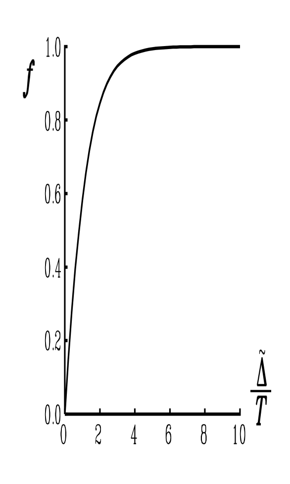
FIG. 3.: The reduction factor $f$ of the Hall conductivity, given by Eq. (143) and shown as a function of the ratio of the energy gap at the Fermi level $\tilde{\Delta}$ to temperature $T$.

The function $f$ (142) depends only on the ratio of the energy gap at the Fermi level, $\tilde{\Delta}$, and the temperature $T$. Introducing the new variable of integration $\zeta$ instead of $k$ via the equation $\hbar v_{F}k=\tilde{\Delta}\sinh\zeta$, we can rewrite Eq. (142) as follows [25, 41]:

$$f\left(\frac{\tilde{\Delta}}{T}\right)=\int_{0}^{\infty}d\zeta\,\frac{\tanh\left(\frac{\tilde{\Delta}}{2T}\cosh\zeta\right)}{\cosh^{2}\zeta}.$$ (143)

The function $f(\tilde{\Delta}/T)$ is plotted in Fig. 3. It is equal to 1 at zero temperature, where Eq. (141) gives QHE, gradually decreases with increasing $T$, and vanishes when $T\gg\tilde{\Delta}$. Taking into account that the FISDW order parameter $\Delta$ itself depends on $T$ and vanishes at the FISDW transition temperature $T_{c}$, it is clear that $f(T)$ and $\sigma_{xy}(T)$ vanish at $T\rightarrow T_{c}$, where $\sigma_{xy}(T)\propto f(T)\propto\Delta(T)\propto\sqrt{T_{c}-T}$. Assuming that the temperature dependence $\tilde{\Delta}(T)$ is given by the BCS theory [10], we plot the temperature dependence of the Hall conductivity, $\sigma_{xy}(T)$, in Fig. 4 [42].

The function $f(T)$ (142) is qualitatively similar to the function $f_{\rm s}(T)$ that describes the temperature reduction of the superconducting condensate density in the London case. Both functions approach 1 at zero temperature, but near $T_{c}$ the superconducting function behaves differently: $f_{\rm s}(T)\propto\Delta^{2}(T)\propto T_{c}-T$. As explained in Sec. VI B, this is due to the difference between the static and dynamic limits of the response function.

FIG. 4.: Hall conductivity in the FISDW state, $\sigma_{xy}$, as a function of temperature $T$ normalized to the FISDW transition temperature $T_{c}$.

In the next Sec. VI A, we give a simple, semiphenomenological derivation of Eqs. (140) and (142) based on the ideas of Refs. [40, 43] and analogous to the standard derivation of the superfluid density (see §27 of Ref. [37]). After that, in Sec. VI B, we give a formal diagrammatic derivation Eqs. (140) and (142). We also derive the effective action of FISDW at a finite temperature.

A Semiphenomenological derivation

Let us consider a 1D electron system where a CDW/SDW of an amplitude $\Delta$ moves with a small velocity $v$. Let us calculate the Fröhlich current, proportional to $v$, at a finite temperature $T$.

We find the electron wave functions in the reference frame moving with the density wave and then Galileo-transform them to the laboratory frame [43]:

$$\psi_{k}^{\pm}(t,x) = u_{k}^{\pm}e^{i(k_{\rm F}+k+mv)x-i(k_{\rm F}+k)vt\mp iE_{k}t/\hbar}$$ (145)

$$+w_{k}^{\pm}e^{i(-k_{\rm F}+k+mv)x-i(-k_{\rm F}+k)vt\mp iE_{k}t/\hbar},$$

where we keep only the terms linear in $v$. In Eq. (145) and below, the index $\pm$ refers to the states above and below the CDW/SDW energy gap, not to the states near $\pm k_{\rm F}$. The coefficients of superposition $u_{k}$ and $w_{k}$ are given by the following expressions:

$$|u_{k}^{+}|^{2}=|w_{k}^{-}|^{2}=\frac{\Delta^{2}}{2E_{k}(E_{k}-\xi_{k})},$$ (146)

$$|w_{k}^{+}|^{2}=|u_{k}^{-}|^{2}=\frac{E_{k}-\xi_{k}}{2E_{k}},$$ (147)

where $\xi_{k}=\hbar v_{F}k$ and $E_{k}=\sqrt{\xi_{k}^{2}+\Delta^{2}}$ are the electron dispersion laws in the absence and in the presence of the CDW/SDW energy gap.

By analogy with the standard derivation of the superfluid density (§27 of Ref. [37]), let us assume that, because of interaction with impurities, phonons, etc., the electron quasiparticles are in thermal equilibrium with the crystal in the laboratory reference frame, so their distribution function is the equilibrium Fermi function $n(E_{k})$. However, it is not straightforward to apply the Fermi function, because the two components of the eigenfunction (145), which have the same energy in the reference frame of the moving CDW/SDW, have different energies in the laboratory frame. Let us make a reasonable assumption that a state (145) is populated according to its average energy $\bar{E}_{k}^{\pm}$:

$$\bar{E}_{k}^{\pm} = |u_{k}^{\pm}|^{2}[\pm E_{k}+\hbar(k_{\rm F}+k)v]$$ (149)

$${}+|w_{k}^{\pm}|[\pm E_{k}+\hbar(-k_{\rm F}+k)v].$$

The electric current $I$ carried by the electrons is equal to

$$I=2e\hbar\sum_{\pm}\int\frac{dk}{2\pi}\,n(\bar{E}_{k}^{\pm})$$ (150)

$$\times\left[|u_{k}^{\pm}|^{2}\left(\frac{k_{F}+k}{m}+\frac{v}{\hbar}\right)+|w_{k}^{\pm}|^{2}\left(\frac{-k_{F}+k}{m}+\frac{v}{\hbar}\right)\right]\!,$$ (151)

where the factor 2 comes from the spin. Substituting Eq. (149) into Eq. (150) and keeping the terms linear in $v$, we find two contributions to $I$. The first contribution, $I_{1}$, is obtained by replacing $\bar{E}_{k}^{\pm}$ with $\pm E_{k}$ in Eq. (150), that is, by omitting $v$ in Eq. (149). This term represents the current produced by all electrons moving with the velocity $v$:

$$I_{1}=2evk_{F}/\pi.$$ (152)

The second contribution $I_{2}$ comes from expansion of the Fermi function in Eq. (150) in $v$ and represents reduction of the current due to thermally excited quasiparticles staying behind the collective motion:

$$I_{2}=2emv\sum_{\pm}\int\frac{dk}{2\pi}\>\frac{\partial n(\pm E_{k})}{\partial E_{k}}$$ (153)

$$\times\left(v_{F}(|u_{k}^{\pm}|^{2}-|w_{k}^{\pm}|^{2})+\frac{\hbar k}{m}(|u_{k}^{\pm}|^{2}+|w_{k}^{\pm}|^{2})\right)^{2}.$$ (154)

The second term in the brackets in Eq. (154) is small compared to the first term and may be neglected. Substituting Eqs. (146) and (147) into Eq. (154) and expressing the CDW/SDW velocity in terms of the CDW/SDW phase derivative in time, $v=-\dot{\tilde{\Theta}}/2k_{F}$, we find the temperature-dependent expression for the Fröhlich current:

$$I=I_{1}+I_{2}=-f(T)\,\frac{e}{\pi}\frac{\partial\tilde{\Theta}}{\partial t},$$ (155)

$$f(T)=1-\int d\xi_{k}\left(\frac{\xi_{k}}{E_{k}}\right)^{\!2}\left(-\frac{\partial n(E_{k})}{\partial E_{k}}\right).$$ (156)

Equation (156) is the same as Eq. (142). Dividing the current per one chain, $I$ (155), by the interchain distance $b$, we get the density of current per unit length, $j_{x}$ (139).

B Diagrammatic derivation

In order to obtain the effective action for FISDW, we repeat the derivation of Sec. V at a finite temperature. Technically, this means that we need to calculate $\Pi^{\mu}$ in Eq. (131) with $\Theta_{0}=0$ at the Matsubara frequencies $i\omega_{n}=i(2n+1)\pi T/\hbar$, then make an analytic continuation to the real frequencies and substitute the result into Eq. (129):

$$\Pi^{\mu}(p,i\Omega_{m})=-\frac{\tilde{\Delta}}{b}\int_{-\infty}^{\infty}\frac{dk}{2\pi}$$ (157)

$$\times T\sum_{n}{\rm Tr}[\tau_{y}{\cal G}(k,i\omega_{n})\tau^{\mu}{\cal G}(k+p,i\omega_{n}+i\Omega_{m})],$$ (158)

where the electron Green function is

$${\cal G}(k,i\omega_{n})=\frac{\tau_{0}i\hbar\omega_{n}+\tau_{z}\hbar v_{F}k+\tau_{x}\tilde{\Delta}}{(i\hbar\omega_{n})^{2}-E_{k}^{2}}.$$ (159)

Substituting Eq. (159) into Eq. (157) and taking the trace, we find

$$\Pi^{\mu}(T,p,i\Omega_{m})=-\varepsilon^{\mu\nu}\frac{ip_{\nu}}{\pi b}\,f(T,p,i\Omega_{m}),$$ (160)

where $p_{\nu}=(i\Omega_{m}/v_{F},-p_{x})$, and

$$f(T,p,i\Omega_{m})=2\tilde{\Delta}^{2}\int_{-\infty}^{\infty}d\xi_{k}$$ (161)

$$\times T\sum_{n}\frac{1}{[(i\hbar\omega_{n})^{2}-E_{k}^{2}][(i\hbar\omega_{n}+i\hbar\Omega_{m})^{2}-E_{k+p}^{2}]}.$$ (162)

The sum (161) is converted into an integral in the complex plane of $\omega$ along a contour encircling the imaginary axis in the counterclockwise direction with the function $-\hbar/T(2\pi i)(e^{\hbar\omega/T}+1)$ multiplying the integrand in Eq. (161). The integral is taken by deforming the contour of integration into four contours encircling the four poles, $\pm E_{k}/\hbar$ and $-i\Omega_{m}\pm E_{k+p}/\hbar$, in the clockwise direction and evaluating the residues. After that, we analytically continue the external Matsubara frequency $i\Omega_{m}$ to the real frequency: $i\Omega_{m}\to\Omega+i\delta$, where $\delta=\epsilon\,{\rm sign}(\Omega)$, and find

$$f(T,p,\Omega)=\frac{1}{2}\int_{-\infty}^{\infty}d\xi_{k}\,\frac{\tilde{\Delta}^{2}}{E_{k}E_{k+p}}$$ (163)

$$\times\left(\frac{n(E_{k+p})+n(E_{k})-1}{\hbar\Omega+i\delta-E_{k}-E_{k+p}}-\frac{n(E_{k+p})+n(E_{k})-1}{\hbar\Omega+i\delta+E_{k}+E_{k+p}}\right.$$ (164)

$$+\left.\frac{n(E_{k+p})-n(E_{k})}{\hbar\Omega+i\delta+E_{k}-E_{k+p}}-\frac{n(E_{k+p})-n(E_{k})}{\hbar\Omega+i\delta-E_{k}+E_{k+p}}\right).$$ (165)

The second line in Eq. (163) contains the sum $E_{k}+E_{k+p}$ in the denominators and describes the interband electron transitions involving the energy greater than $2\tilde{\Delta}$. On the other hand, the third line in Eq. (163) contains the difference $E_{k}-E_{k+p}$ in the denominators and describes the intraband electron transitions within the same energy band.

Substituting Eq. (160) into Eq. (129) and taking the variational integral over $\delta\tilde{\Theta}$, we find that the effective action of FISDW at a finite temperature has the form (113) and (116), Fourier-transformed from $(t,x)$ to $(p,\Omega)$ and multiplied by the temperature-dependent factor $f(T,p,\Omega)$ (163). Since Lagrangian (116) represents an expansion in the powers of small gradients, we would like to take the limit of $p\to 0$ and $\Omega\to 0$ in $f(T,p,\Omega)$. However, at a finite temperature, the result depends on the order of limits. In the dynamic limit, $\Omega\gg\hbar v_{F}p$, where we take the limit $p\to 0$ before $\Omega\to 0$, the intraband cluster [the third line of Eq. (163)] gives no contribution, while the interband cluster (the second line) gives

$$f_{d}(T) = \lim_{\Omega\to 0}\lim_{p\to 0}f(T,p,\Omega)$$ (166)

$$= \int_{-\infty}^{\infty}d\xi_{k}\left(\frac{\tilde{\Delta}}{E_{k}}\right)^{2}\frac{1-2n(E_{k})}{E_{k}}$$ (167)

$$= 1-\int_{-\infty}^{\infty}d\xi_{k}\left(\frac{\xi_{k}}{E_{k}}\right)^{2}\left(-\frac{\partial n(E_{k})}{\partial E_{k}}\right).$$ (168)

The integral of the first term in Eq. (167) gives 1 in Eq. (168), and the second term in Eq. (167), integrated by parts, gives the second term in Eq. (168). The function $f_{d}(T)$ in the dynamical limit (168) is the same as the function $f(T)$ (156) derived semiphenomenologically in Sec. VI A. The dynamic limit is appropriate for calculating electric conductivity, including the Hall conductivity, when the electric field and FISDW are strictly homogeneous in space ($p=0$), but may be time-dependent ($\Omega\neq 0$). Thus, the ac Hall conductivity at a finite temperature is given by Eq. (17) and Fig. 1 multiplied by $f(T)=f_{d}(T)$.

The function $f_{s}(T)$ in the static limit, $\Omega\ll\hbar v_{F}p$, is obtained from $f_{d}(T)$ (168) by adding the intraband contribution:

$$f_{s}(T) = \lim_{p\to 0}\lim_{\Omega\to 0}f(T,p,\Omega)$$ (169)

$$= f_{d}(T)-\int_{-\infty}^{\infty}d\xi_{k}\left(\frac{{\tilde{\Delta}}}{E_{k}}\right)^{2}\left(-\frac{\partial n(E_{k})}{\partial E_{k}}\right).$$ (170)

Combining the second term in Eq. (168) with the last term in Eq. (170), we find

$$f_{s}(T)=1-\int_{-\infty}^{\infty}d\xi_{k}\left(-\frac{\partial n(E_{k})}{\partial E_{k}}\right).$$ (171)

The function $f_{s}(T)$ in the static limit is the same as the function that determines the temperature reduction of the superfluid condensate density in London superconductors, $\rho_{s}(T)/\rho$, [44]. This quantity controls the Meissner effect and, thus, determines the temperature dependence of the magnetic field penetration depth in superconductors. It also controls the charge-density response to a static deformation of the CDW phase, $\partial\Theta/\partial x$ [40, 41]. The static limit is appropriate in these cases, because the CDW phase or the magnetic field in the Meissner effect are stationary ($\Omega=0$), but vary in space ($p\neq 0$). Different, but equivalent expressions for $f_{d}(T)$ and $f_{s}(T)$ were obtained in Ref. [41] by integrating over the internal momentum of the loop, $k$, in Eq. (163) first.

Comparing the definition (160) of the function $f$ with Eqs. (131), (133), and (136), we find that at zero temperature $f=-C/2$, where $C$ is the Chern number. At zero temperature, the last terms in Eqs. (168) and (171) vanish, so that $f_{d}(T=0)=f_{s}(T=0)=1$, which agrees with the value $-2$ of the Chern number (137). We may think of $-2f(T)$ as a generalization of the Chern number to a finite temperature, where it is not an integer topological invariant any more, because of discrete summation, instead of integration, over the frequency $\omega$.

The dependence of the function $f(T,p,\Omega)$ on the order of limits indicates that the function is not analytic at small $p$ and $\Omega$. Thus, at $T\neq 0$, the effective Lagrangian of the system cannot be written in a local form in the coordinate space as an expansion in powers of gradients for an arbitrary relation between the time and space gradients, so the momentum representation should be used. For the finite-temperature (2+1)D Chern-Simons theory this was emphasized in Refs. [45, 46]. Another finite-temperature effect is dissipation, which manifests itself as the imaginary part of $f(T,p,\Omega)$ appearing at $\Omega\leq v_{F}p$. This Landau damping, originating from the intraband electron transitions, is also known in the theory of CDW/SDW [30] and superconductivity [47].

VII EXPERIMENTAL IMPLICATIONS

In this paper, we predict two specific functions that can be measured experimentally. One is the frequency dependence (Fig. 1) and another is the temperature dependence (Fig. 4) of the Hall conductivity.

The temperature dependence of the Hall resistivity in (TMTSF)₂PF₆ was measured in experiments [48, 49]. However, to compare the experimental results with our Eqs. (141)–(143) for $\sigma_{xy}(T)$, it is necessary to convert the Hall resistivity into the Hall conductivity, which requires experimental knowledge of all components of the resistivity tensor. Only the temperature dependences of $\rho_{xx}$ and $\rho_{xy}$, but not $\rho_{yy}$, were measured in Refs. [48, 49]. Measuring the temperature dependences of all three components of the resistivity tensor and reconstructing $\sigma_{xy}(T)$ would play the same role for QHE as measuring the temperature dependences of the magnetic-field penetration depth for superconductors.

The frequency dependence of the Hall conductivity in regular semiconductor QHE systems was measured using the technique of crossed wave guides [50, 51]. Unfortunately, no such measurements were performed in the FISDW systems. These measurements would be very interesting, because they would reveal the competition between the FISDW motion and QHE. The required frequency should exceed the FISDW pinning frequency $\omega_{0}$ and the damping rate $1/\tau$. To give a crude estimate of the required frequency range, we quote the value of the pinning frequency $\omega_{0}\sim$ 3 GHz $\sim$ 0.1 K $\sim$ 10 cm for a regular SDW (not FISDW) in (TMTSF)₂PF₆ [52]. One would expect a smaller value for FISDW.

FISDW can be depinned not only by an ac electric field, but also by a strong dc electric field. The FISDW depinning and the influence of steady FISDW sliding on the Hall effect were observed experimentally in Refs. [53, 54, 55]. Because the steady sliding of a density wave is controlled by dissipation, it is difficult to interpret these experiments quantitatively within a microscopic theory. According to our theory, in the dc case, the nontrivial terms that couple the $x$ and $y$ directions along and across the chains [the last terms in Eqs. (14) and (16) proportional to $\ddot{\Theta}$ and $\dot{\cal E}_{y}$] vanish. Thus, the only effect of the FISDW sliding is an additional Fröhlich current along the chains, $\Delta j_{x}$, which is a nonlinear function of ${\cal E}_{x}$. In other words, the main effect of the dc FISDW sliding would be a nonlinear increase in $\sigma_{xx}$ and, possibly, in $\sigma_{yy}$ via increasing the number of excited nonequilibrium quasiparticles, but we would expect no major effect on $\sigma_{xy}$. Nevertheless, the dc FISDW sliding would affect the experimentally measured Hall resistivity, because $\rho_{xy}$ depends on all components of the conductivity tensor.

On a more subtle level, in the presence of a magnetic field, one could phenomenologically add a term proportional to $E_{y}$ to Eq. (16) and a term proportional to $\dot{\Theta}$ to Eq. (14). These terms would directly modify $\sigma_{xy}$ for the dc sliding of FISDW. Because these terms violate the time-reversal symmetry of the equations, their nature must be dissipative. Thus, they cannot be derived within the Lagrangian formalism, employed in this paper, and should be obtained from the Boltzmann equation, where the time-reversal symmetry is already broken. The steady motion of the density-wave condensate itself does not contribute to the Hall effect; however, this motion influences the thermally excited normal carriers and, in this way, affects the Hall voltage. This picture is complimentary to our theory, which studies only the condensate contribution. Because the normal carriers need to be thermally excited across the FISDW energy gap, we expect these dissipative terms to be exponentially small and negligible at low temperatures.

The influence of steady sliding of a regular CDW on the Hall conductivity was studied theoretically in Ref. [56] along the lines explained in the preceding paragraph. Since the bare value of the Hall conductivity in a regular CDW/SDW system is determined by the normal carriers only, the steady motion of the density wave produces a considerable, of the order of unity, effect on the Hall conductivity, which was observed experimentally [57]. On the other hand, in the case of the FISDW, where the big quantum contribution from the electrons below the gap dominates the Hall conductivity, the contribution of the thermally excited normal carriers to the Hall conductivity should be negligible at low temperatures.

VIII CONCLUSIONS

In this paper, we have derived the effective Lagrangian (116), equivalently represented by Eq. (119), for free FISDW. The effective Lagrangian (119) consists of the (2+1)D Chern-Simons term and the (1+1)D chiral-anomaly term, both written for the effective field $A^{i}+a^{i}$, where $A^{i}$ is an external electromagnetic field, and $a^{i}$ is the chiral field (37) associated with the gradients of FISDW. When FISDW is pinned, this effective Lagrangian produces QHE. On the other hand, in the ideal case where FISDW is free, the counterflow of FISDW precisely cancels the quantum Hall current, so the resultant Hall conductivity is zero. The ac Hall conductivity $\sigma_{xy}(\omega)$ (17) interpolates between these two limits at low and high frequencies, as shown in Fig. 1.

At a finite temperature, the effective Lagrangian (116) or (119) should be multiplied by the function $f(T,p,\Omega)$ given by Eq. (163), which has the dynamic and static limits $f_{d}(T)$ (168) and $f_{s}(T)$ (171). The dynamic limit determines the temperature dependence of the Hall conductivity, which is given by Eqs. (141)–(143) and shown in Fig. 4. By analogy with the BCS theory of superconductivity, this temperature dependence can be interpreted within the two-fluid picture of QHE, where the Hall conductivity of the condensate is quantized, but the condensate fraction of the total electron density decreases with increasing temperature.

Experimentalists are urged to measure the frequency and temperature dependences of $\sigma_{xy}$ in the FISDW state of the (TMTSF)₂X materials.

In this appendix we calculate the Chern number (137):

$$C=\int\frac{dk\,d\omega\,d\Theta_{0}}{4\pi^{2}}{\rm Tr}\left(\frac{\partial{\cal G}_{0}^{-1}}{\partial\Theta_{0}}{\cal G}_{0}\frac{\partial{\cal G}_{0}^{-1}}{\partial\omega}{\cal G}_{0}\frac{\partial{\cal G}_{0}^{-1}}{\partial k}{\cal G}_{0}\right).$$ (172)

In Eq. (172) we added the index 0 to the Green functions ${\cal G}_{0}$ in order to remind that they depend on the constant phase $\Theta_{0}$ via the substitution $\Delta\to\tilde{\Delta}\exp(-i\tau_{z}\Theta_{0})$ in Eq. (40). Now let us make a unitary transformation that eliminates the phase $\Theta_{0}$ from the Green functions:

$$U^{+}{\cal G}_{0}U={\cal G},\quad U=e^{i\tau_{z}\Theta_{0}/2},$$ (173)

where ${\cal G}$ is given by Eq. (40) with $\Delta\to\tilde{\Delta}$. Substituting Eq. (173) into Eq. (172) and taking into account that $\partial{\cal G}^{-1}/\partial\omega=\hbar$, we find

$$C=\hbar\int\frac{dk\,d\omega\,d\Theta_{0}}{4\pi^{2}}{\rm Tr}\left(U^{+}\frac{\partial(U{\cal G}^{-1}U^{+})}{\partial\Theta_{0}}U{\cal G}{\cal G}\frac{\partial{\cal G}^{-1}}{\partial k}{\cal G}\right).$$ (174)

Since ${\cal G}$ does not depend on $\Theta_{0}$, we need to differentiate only the matrices $U$ and $U^{+}$ in Eq, (174), which gives the following two terms:

$$C=i\frac{\hbar}{2}\int\frac{dk\,d\omega\,d\Theta_{0}}{4\pi^{2}}{\rm Tr}\left(\tau_{z}{\cal G}\frac{\partial{\cal G}^{-1}}{\partial k}{\cal G}-{\cal G}{\cal G}\frac{\partial{\cal G}^{-1}}{\partial k}\tau_{z}\right).$$ (175)

The second term in Eq. (175) is proportional to $P^{00}$ (45) and vanishes according to Eq. (51), whereas the first term is proportional to $P^{11}$ (50). Using Eqs. (48) and (41), we find the value of $C$:

$$C = -i\frac{\hbar}{2}\int\frac{dk\,d\omega}{2\pi}{\rm Tr}\left(\tau_{z}\frac{\partial{\cal G}}{\partial k}\right)$$ (176)

$$= \int dk\,\frac{\partial[n_{+}(k)-n_{-}(k)]}{\partial k}=-2.$$ (177)

For spinless fermions, the number in Eq. (177) would be $-1$.

REFERENCES

- [1] Electronic address: yakovenk@physics.umd.edu.
- [2] Electronic address: goan@physics.umd.edu.
- [3] T. Ishiguro and K. Yamaji, Organic Superconductors (Springer-Verlag, Berlin, 1990).
- [4] D. Jérome, in Organic Conductors: Fundamentals and Applications, edited by J.-P. Farges (Marcel Dekker, New York, 1994).
- [5] P. M. Chaikin, J. Phys. I (Paris) 6, 1875 (1996).
- [6] L. P. Gor’kov and A. G. Lebed’, J. Phys. Lett. (Paris) 45, L433 (1984).
- [7] A. G. Lebed’, Zh. Eksp. Teor. Fiz. 89, 1034 (1985) [Sov. Phys. JETP 62, 595 (1985)].
- [8] M. Héritier, G. Montambaux, and P. Lederer, J. Phys. Lett. (Paris) 45, L943 (1984).
- [9] G. Montambaux, M. Héritier, and P. Lederer, Phys. Rev. Lett. 55, 2078 (1985).
- [10] D. Poilblanc, M. Héritier, G. Montambaux and P. Lederer, J. Phys. C 19, L321 (1986).
- [11] G. Montambaux and D. Poilblanc, Phys. Rev. B 37, 1913 (1988).
- [12] K. Yamaji, J. Phys. Soc. Jpn. 54, 1034 (1985).
- [13] K. Maki, Phys. Rev. B 33, 4826 (1986).
- [14] A. Virosztek, L. Chen, and K. Maki, Phys. Rev. B 34, 3371 (1986).
- [15] L. Chen and K. Maki, Phys. Rev. B 35, 8462 (1987).
- [16] G. Montambaux, Phys. Scr. T 35, 188 (1991).
- [17] P. Lederer, J. Phys. I (Paris) 6, 1899 (1996).
- [18] D. Poilblanc, G. Montambaux, M. Héritier, and P. Lederer, Phys. Rev. Lett. 58, 270 (1987).
- [19] V. M. Yakovenko, Phys. Rev. B 43, 11353 (1991).
- [20] K. Machida, Y. Hasegawa, M. Kohmoto, V. M. Yakovenko, Y. Hori, and K. Kishigi, Phys. Rev. B 50, 921 (1994).
- [21] V. M. Yakovenko and H.-S. Goan, J. Phys. I (Paris) 6, 1917 (1996).
- [22] D. J. Thouless in The Quantum Hall Effect, edited by R. E. Prange and S. M. Girvin (Springer, New York, 1987), p. 101.
- [23] G. Grüner, Rev. Mod. Phys. 60, 1129 (1988); 66, 1 (1994); Density Waves in Solids (Addison-Wesley, New York, 1994).
- [24] P. B. Wiegmann, Prog. Theor. Phys. 107, 223 (1992); in Field Theory, Topology, and Condensed Matter Systems, edited by H. Geyer (Springer, New York, 1995).
- [25] A. Virosztek and K. Maki, Phys. Rev. B 39, 616 (1989).
- [26] T. G. Petrova and A. S. Rozhavsky, Fiz. Nizk. Temp. 18, 987 (1992) [Sov. J. Low Temp. Phys. 18, 692 (1992)]; J. Phys. IV (Paris), Colloque C2, 3, 303 (1993); A. S. Rozhavsky, Int J. Mod. Phys. B 7, 3415 (1993).
- [27] V. M. Yakovenko, J. Phys. IV (Paris), Colloque C2, 3, 307 (1993); J. Supercond. 7, 683 (1994); V. M. Yakovenko and H.-S. Goan, in Proceedings of the Physical Phenomena at High Magnetic Fields–II Conference, edited by Z. Fisk et al. (World Scientific, Singapore, 1996), p. 116; Synth. Met. 85, 1609 (1997).
- [28] I. V. Krive and A. S. Rozhavsky, Phys. Lett. A 113, 313 (1985).
- [29] Z.-B. Su and B. Sakita, Phys. Rev. Lett. 56, 780 (1986); Phys. Rev. B 38, 7421 (1988); B. Sakita and Z.-B. Su, Progr. Theor. Phys. Suppl. 86, 238 (1986).
- [30] S. Brazovskii, J. Phys. I (Paris) 3, 2417 (1993).
- [31] M. Ishikawa and H. Takayama, Progr. Theor. Phys. 79, 359 (1988).
- [32] R. B. Laughlin, Phys. Rev. B 23, 5632 (1981).
- [33] I. Dana, Y. Avron, and J. Zak, J. Phys. C 18, L679 (1985).
- [34] L. D. Landau and E. M. Lifshitz, The Classical Theory of Fields (Pergamon, Oxford, 1994).
- [35] The subscript and superscript indices should not be confused with imaginary number , the current , and the wave vector .
- [36] S. A. Brazovskii and I. E. Dzyaloshinskii, Zh. Eksp. Teor. Fiz. 71, 2338 (1976) [Sov. Phys. JETP 44, 1233 (1976)].
- [37] E. M. Lifshitz and L. P. Pitaevskii, Statistical Physics, Part 2 (Pergamon, Oxford, 1991).
- [38] More precisely, transformation (101) should be done in two steps. First we transform the fermions in the momentum representation: . Then we go from the momentum to the coordinate representation in and do the second transformation . In this way we can accommodate the dependence of on .
- [39] In our derivation, we neglected the terms proportional to , , and in the effective Lagrangian (116). These terms describe polarizability and magnetic susceptibility, but are not essential for calculating conductivity.
- [40] P. A. Lee and T. M. Rice, Phys. Rev. B 19, 3970 (1979); T. M. Rice, P. A. Lee, and M. C. Cross ibid., 20, 1345 (1979).
- [41] K. Maki and A. Virosztek, Phys. Rev. B 41, 557 (1990); 42, 655 (1990).
- [42] Strictly speaking, Eq. (141) gives only the Hall effect of the FISDW condensate and should be supplemented with the Hall conductivity of thermally excited normal carriers. Then, at , should not vanish, but approach to the Hall conductivity of the metallic phase. The latter is determined by the distribution of the electron scattering time over the Fermi surface and is small. The curve shown in Fig. 4 should be modified accordingly in a narrow vicinity of .
- [43] M. L. Boriack and A. W. Overhauser, Phys. Rev. B 15, 2847 (1977); 16, 5206 (1977); 17, 2395 (1978).
- [44] A. L. Fetter and J. D. Walecka, Quantum Theory of Many-Particle Systems (McGraw-Hill, New York, 1971), pp. 459–460.
- [45] Y.-C. Kao and M.-F. Yang, Phys. Rev. D 47, 730 (1993).
- [46] I. J. R. Aitchison and J. A. Zuk, Ann. Phys. (NY) 242, 77 (1995).
- [47] E. Abrahams and T. Tsuneto, Phys. Rev. 152, 416 (1966).
- [48] W. Kang et al., Phys. Rev. B 45, 13566 (1992).
- [49] S. Valfells et al., Phys. Rev. B 54, 16413 (1996).
- [50] F. Kuchar et al., Phys. Rev. B 33, 2965 (1986).
- [51] L. A. Galchenkov et al., Pis’ma Zh. Eksp. Teor. Fiz. 46, 430 (1987) [JETP Lett. 46, 542 (1987)].
- [52] D. Quinlivan et al., Phys. Rev. Lett. 65, 1816 (1990).
- [53] T. Osada et al., Phys. Rev. Lett. 58, 1563 (1987).
- [54] L. Balicas, N. Biškup, and G. Kriza, J. Phys. IV (Paris), Colloque C2, 3, 319 (1993).
- [55] L. Balicas, Phys. Rev. Lett. 80, 1960 (1998).
- [56] S. N. Artemenko and A. N. Kruglov, Fiz. Tverd. Tela 26, 2391 (1984) [Sov. Phys. Solid State 26, 1448 (1984)]; E. N. Dolgov, Fiz. Nizk. Temp. 10, 911 (1984) [Sov. J. Low Temp. Phys. 10, 474 (1984)].
- [57] S. N. Artemenko et al., Pis’ma Zh. Eksp. Teor. Fiz. 39, 258 (1984) [JETP Lett. 39, 308 (1984)]; L. Forró et al., Phys. Rev. B 34, 9047 (1986); L. Forró et al., Solid State Commun. 62, 715 (1987); O. Trætteberg, L. Balicas, and G. Kriza, J. Phys. IV (Paris), Colloque C2, 3, 61 (1993).