Atomic Scattering in Presence of an External Confinement
and a Gas of Impenetrable Bosons

Abstract

We calculate, within the pseudopotential approximation, a one-dimensional scattering amplitude and effective one-dimensional interaction potential for atoms confined transversally by an atom waveguide or highly elongated “cigar”-shaped atomic trap. We show that in the low-energy scattering regime, the scattering process degenerates to a total reflection suggesting an experimental realization of a famous model in theoretical physics - a one-dimensional gas of impenetrable bosons (“Tonks” gas). We give an estimate for suitable experimental parameters for alkali atoms confined in waveguides.

Rapid progress in producing Bose condensates of alkali atoms [1] opened up new areas of ultra-low energy collisional physics. Concurrently, work has progressed on confinement of atoms in the light-induced [2] and magnetic-field-induced [3] atom waveguides.

We develop a theory for the binary atomic collisions in presence of a transverse external confinement. Using the pseudopotential approximation, we derive an expression for an effective one-dimensional scattering amplitude and show that the interparticle interaction can be approximated by an effective one-dimensional $\delta$-potential of a known strength. In the case of a dilute atomic gas, when the three body collisions are negligible, our effective potential can also be used to describe quasi-one-dimensional many-body systems: a project on the experimental realization of the one-dimensional Bose condensate is already presented in the literature [4]. Results of our paper will allow one to properly take into account the trap-induced corrections to the strength of the atomic mean-field potential.

Furthermore, we show that in the low-energy scattering limit ($k_{z}|a_{\rm 1D}|\ll 1$), the effective one-dimensional scattering degenerates to a total reflection ($\hbar k_{z}$ is the longitudinal component of the atomic momentum and $a_{\rm 1D}$ is the one-dimensional scattering length defined below). This conclusion allows us to suggest an experimental realization of another famous model in theoretical physics – a one-dimensional gas of impenetrable bosons [5] also referred to as a “Tonks” gas. Such a system provides us with an unusual example of a boson-fermion duality: the elementary excitations of such a bosonic system obey Fermi statistics [6] (which is possible only in one dimension [7]). The Tonks gas is, therefore, a system complementary to the one-dimensional Bose condensate: the latter requires the high-energy scattering regime ($k_{z}|a_{\rm 1D}|\gg 1$) [8] and its excitation spectrum is represented by the Bogoliubov bosons.

To describe the binary collisions between cold atoms confined in a waveguide, we suggest the following model:

  

(a) The waveguide potential is replaced by an axially symmetric 2D harmonic potential of a frequency $\omega_{\perp}$. The forces created by the potential act along the X-Y plane;

  

(b) Atomic motion along the Z axis is free;

  

(c) Interaction between the atoms is modeled by the Huang’s pseudopotential [9]

$$U(r)=g\delta({\bf r})\,\frac{\partial}{\partial r}(r\,\cdot\,)\,\,,$$ (1)

where $g=2\pi\hbar^{2}a/\mu$ is the potential strength, $a$ is the $s$-wave scattering length for the “true” interaction potential, $\mu=m/2$ is the reduced mass, $m$ is the mass of the atoms. The regularization operator $\frac{\partial}{\partial r}(r\,\cdot\,)$, that removes the $1/r$ divergence from the scattered wave (see [9]), plays an important role in the derivation below;

  

(d) Atomic motion (both transverse and longitudinal components) is “cooled down” below the transverse vibrational energy $\hbar\omega_{\perp}$. We will justify this condition in the second subsequent paragraph.

The harmonic nature of the confining potential allows the separation of the center-of-mass and relative motions. The Schrödinger equation governing the relative motion reads

$$\left\{\frac{\hat{p}_{z}^{2}}{2\mu}+g\delta({\bf r})\,\frac{\partial}{\partial r}(r\,\cdot\,)+\hat{H}_{\perp}(\hat{p}_{x},\hat{p}_{y},x,y)\right\}\Psi=E\Psi\,,$$ (2)

where ${\bf r}={\bf r_{2}}-{\bf r_{1}}$ is a relative coordinate for atoms $1$ and $2$ and

$$\hat{H}_{\perp}=\frac{\hat{p}_{x}^{2}+\hat{p}_{y}^{2}}{2\mu}+\frac{\mu\omega_{\perp}^{2}(x^{2}+y^{2})}{2}$$ (3)

is a 2D harmonic oscillator Hamiltonian.

We will suppose that (i) the incident wave $e^{ik_{z}z}\phi_{n=0,m_{z}=0}(\rho)$ corresponds to a particle in the ground state of the transverse Hamiltonian (3) ($\rho=\sqrt{x^{2}+y^{2}}$), and (ii) the longitudinal kinetic energy of the incident wave is limited by the energy spacing between the ground and first axially symmetric excited state:

$$\frac{\hbar^{2}k_{z}^{2}}{2\mu}<E_{n=2,m_{z}=0}-E_{n=0,m_{z}=0}=2\hbar\omega_{\perp}\,.$$ (4)

Here $E_{n,m_{z}}=\hbar\omega_{\perp}(n+1)$ is the energy spectrum of the 2D harmonic oscillator, $n=0,1,2,\ldots,\infty$ is the principal quantum number, $m_{z}$ is the angular momentum with respect to the Z axis, $m_{z}=0,2,4,\ldots,n\,(1,3,5,\ldots,n)$ if $n$ is even(odd). The asymptotic form of the scattering wave function $\Psi$ then reads

$$\Psi(z,\rho)\stackrel{{\scriptstyle|z|\rightarrow\infty}}{{\longrightarrow}}$$ (5)

$$\left\{\,e^{ik_{z}z}+f_{\rm even}\,e^{ik_{z}|z|}+f_{\rm odd}\,{\rm sign}(z)e^{ik_{z}|z|}\,\right\}\,\phi_{0,0}(\rho)\,,$$ (6)

where the first term in the curly brackets represents the incident wave, the second and third terms give the even and odd scattered waves respectively, and $f_{\rm even}(k_{z})$ and $f_{\rm odd}(k_{z})$ are the one-dimensional scattering amplitudes for the even and odd partial waves respectively. Note that the transverse state ($n=0,\,m_{z}=0$) remains unchanged after the collision. Transitions to the higher ($n>0$) modes are forbidden due to either angular momentum or energy conservation (if the condition (4) is satisfied). We would like to stress however, that during the collision itself a virtual excitation of the high energy axially symmetric modes ($n>0,\,m_{z}=0$) is not forbidden and it is properly taken into account below. One of the goals of this paper is to calculate the amplitudes (6).

For the zero-range potential (1) the one-dimensional scattering amplitudes (6) can be calculated analytically. To perform this calculation we expand the wave function $\Psi(z,\rho)$ to a series over the eigenstates of the transverse Hamiltonian (3), substitute the expansion into the Schrödinger equation (2) using $E=\hbar^{2}k_{z}^{2}/2\mu+\hbar\omega_{\perp}$ for the energy in the right hand side, and then apply the asymptotic conditions (6) along with the conditions of the continuity of the wave function and its derivative. We obtain the following expression for the scattering amplitudes:

$$f_{\rm even}=-\,\frac{i\mu}{\hbar^{2}k_{z}}\phi_{0,0}^{*}(0)g\eta\,\,\,\,\,\,;\,\,\,\,\,\,f_{\rm odd}=0\,\,,$$ (7)

where $\eta$ is the $r\rightarrow 0$ limit of the regular (free of the $1/r$ divergence) part of the solution $\Psi$:

$$\eta=\frac{\partial}{\partial r}[r\,\Psi({\bf r})]\Big{|}_{r\rightarrow 0}=\frac{\partial}{\partial z}[z\,\Psi(z,\rho=0)]\Big{|}_{z\rightarrow 0+}\,\,\,\,.$$ (8)

The expression for the wave function reads

$$\Psi(z,\rho=0) = \frac{1}{\sqrt{\pi}a_{\perp}}\exp(ik_{z}z)$$ (9)

$$- \frac{ig\mu\eta}{\pi\hbar^{2}k_{z}a_{\perp}^{2}}\exp(ik_{z}|z|)$$ (10)

$$- \frac{g\mu\eta}{2\pi\hbar^{2}a_{\perp}}\Lambda\left[\frac{2|z|}{a_{\perp}},\,-\left(\frac{k_{z}a_{\perp}}{2}\right)^{2}\right]\,,$$ (11)

where the function $\Lambda$ is defined as $\Lambda[\xi,\,\epsilon]=\sum_{s^{\prime}=1}^{\infty}\exp(-\sqrt{s^{\prime}+\epsilon}\,\xi)/\sqrt{s^{\prime}+\epsilon}$ [11], the sum over $s^{\prime}=n/2$ originates from a sum $\sum_{n=0,2,4,\ldots}^{\infty}\ldots\,\,$ over the transverse states $\phi_{n,m_{z}=0}$, and $a_{\perp}=(\hbar/\mu\omega_{\perp})^{1/2}$ is the size of the ground state $\phi_{n=0,m_{z}=0}$ of transverse Hamiltonian (3). Above we have used a simple relation $|\phi_{n,m_{z}=0}(\rho=0)|^{2}=1/\pi a_{\perp}^{2}$ for the wave functions of the 2D harmonic oscillator. The value $\phi_{0,0}(\rho=0)$ has been chosen to be real and positive.

The regular part $\eta$ of the wave function is not explicitly defined yet, being a solution of the equation (8). Note that the order of the partial derivative $\partial/\partial z$ and the sum over $s^{\prime}$ in the $\Lambda$-function can not be interchanged because the series $\Lambda$ does not converge uniformly as $\xi\rightarrow 0$. The value of $\eta$ can be extracted from the equation (8) using the following expansion for the function $\Lambda$: $\Lambda[\xi,\,\epsilon]=2/\xi+{\cal L}(\epsilon)+{\cal L}_{1}(\epsilon)\xi+\ldots\,\,$, where the zero-order term of the expansion has a form ${\cal L}(\epsilon)=-\,{\cal C}+\bar{\cal L}(\epsilon)$ and

$${\cal C} =\lim_{s\rightarrow\infty}\,\left(\int_{0}^{s}\frac{d\,s^{\prime}}{\sqrt{s^{\prime}}}-\sum_{s^{\prime}=1}^{s}\,\frac{1}{\sqrt{s^{\prime}}}\right)=1.4603\ldots\,\,\,,$$ (12)

$$\bar{\cal L} (\epsilon)=\sum_{n=1}^{\infty}(-1)^{n}\,\frac{{\zeta}[(1+2n)/2](2n-1)!!\,\epsilon^{n}}{2^{n}n!}\,\,.$$ (13)

To prove this formula one should subtract and add a sum $\sum_{s^{\prime}=1}^{\infty}\int_{s^{\prime}-1}^{s^{\prime}}\,ds^{\prime\prime}\,\exp(-\sqrt{s^{\prime\prime}}\xi)/\sqrt{s^{\prime\prime}}=2/\xi$ to the function $\Lambda$. The sum of the differences between the $\Lambda$ terms and the terms of the above sum converges uniformly and the derivative in (8) can be easily calculated. Here ${\zeta}[\xi]$ is the Riemann zeta-function.

We now write down the final expression for the one-dimensional scattering amplitude (6):

$$f_{\rm even}(k_{z})=$$ (15)

$$-\,\frac{1}{1+ik_{z}a_{\rm 1D}-\underbrace{(ik_{z}a_{\perp}/2)\,\,\bar{\cal L}(-k_{z}^{2}a_{\perp}^{2}/4)}_{{\cal O}((k_{z}a_{\perp})^{3})}}\,\,\,\,\,\,,$$

where the function $\bar{\cal L}(\epsilon)$ is given by (13). Here

$$a_{\rm 1D}=-\frac{a_{\perp}^{2}}{2a}\,\left(1-{\cal C}\frac{a}{a_{\perp}}\right)$$ (16)

is the one-dimensional scattering length and the constant ${\cal C}$ is given by (12). In analogy with three-dimensional scattering, the one-dimensional scattering length is defined as a derivative $-\partial\Delta/\partial k_{z}|_{k_{z}\rightarrow 0+}$ of the even-wave scattering phase. The scattering phase $\Delta(k_{z})$ is defined through the even solution $\Psi\propto\sin[k_{z}|z|+\Delta(k_{z})]\phi_{0,0}(\rho)$ of the Schrödinger equation (2). The formula for the one-dimensional scattering amplitude (15) is the key result of this paper.

The expression (15) is valid for any strength of the transverse confinement. Note however, that the tight confinement limit $a_{\perp}\ll|a|$ makes sense only if the $s$-wave scattering amplitude for the “true” 3D finite-range interatomic potential (approximated in this paper by the Huang’s pseudopotential (1)) shows a zero-energy resonance; namely if the $s$-wave scattering length $a$ (the same for both potentials) is much greater than the effective range $r_{0}$ of the “true” potential [10]. Indeed the 3D pseudopotential approximation (1) is only valid for velocities which are lower then the inverted effective range ($k\ll r_{0}^{-1}$) (see [12]), and therefore requires a lower bound for the transverse size: $a_{\perp}\sim k_{\perp}^{-1}\gg r_{0}$. This condition and the tight confinement regime criterion ($a_{\perp}\ll|a|$) are consistent only in the resonant case: $|a|\gg r_{0}$.

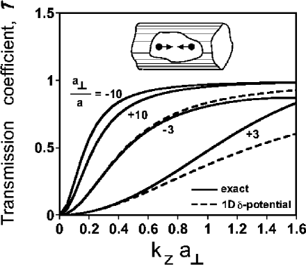
FIG. 1.: Transmission probability as a function of the incident momentum. Solid lines correspond to the exact 1D scattering amplitude (15). Dashed lines correspond to the 1D $\delta$-potential approximation $f_{\rm even}\approx f_{\rm even}^{\delta}$. For $a_{\perp}/a=\pm 10$ the result of the $\delta$-potential approximation almost coincides with the exact amplitude and is not shown.

For low velocities the exact scattering amplitude (15) can be approximated by a scattering amplitude $f_{\rm even}^{\delta}(k_{z})=-1/(1+ik_{z}a_{\rm 1D})$ for a one-dimensional $\delta$-potential

$$U_{\rm 1D}(z)=g_{\rm 1D}\delta(z)$$ (17)

of a coupling strength

$$g_{\rm 1D}=-\,\frac{\hbar^{2}}{\mu\,a_{\rm 1D}}=g\,|\phi_{0,0}(0)|^{2}\,\left(1-{\cal C}\frac{a}{a_{\perp}}\right)^{-1}\,,$$ (18)

where $|\phi_{0,0}(0)|^{2}=1/\pi a_{\perp}^{2}$. To illustrate this statement we plot (Fig.1) the transmission coefficient ${\cal T}=|1+f_{\rm even}+f_{\rm odd}|^{2}$ calculated using the exact scattering amplitude (15) along with the results of the 1D $\delta$-potential approximation $f_{\rm even}\approx f_{\rm even}^{\delta}$. Recall that in both cases the odd-wave scattering amplitude vanishes: $f_{\rm odd}=f_{\rm odd}^{\delta}=0$.

The effective potential (17,18) can be shown to reproduce the low-energy scattering properties of the radius $a$ hard spheres in presence of a transverse trap. Recall that the Huang’s potential (1) plays exactly the same role in the free space. By analogy with the “free-space” case [9], the the limits of applicability of our potential can be extended to the many-body problems to describe interactions between the atoms confined to the ground transverse state.

Note that the one-dimensional gas of bosons interacting via a $\delta$-potential is already widely investigated in theoretical physics [13]. One of the most interesting models belonging to this class is a one-dimensional gas of impenetrable bosons. Formally this model corresponds to the infinitely strong repulsive interaction between atoms: $g_{\rm 1D}\rightarrow+\infty$. More rigorously the impenetrable bosons regime corresponds to the low-energy scattering limit

$$k_{z}|a_{\rm 1D}|\ll 1$$ (19)

when the corresponding transmission coefficient ${\cal T}$ approaches zero (see Fig.1). (Recall that for positive interaction strength $g_{\rm 1D}$ the corresponding one-dimensional scattering length $a_{\rm 1D}$ is negative.) A remarkable feature of the gas of impenetrable bosons is a possibility of a one-to-one mapping between the bosonic system and a gas of noninteracting fermions.

For $N$ impenetrable bosons confined in a periodic-boundary-conditions one-dimensional box of a length $L$ the ground state of the system $\Psi^{b}$ is given by an absolute value of the ground state of the $N$-particle ideal Fermi gas:

$$\Psi^{b}=\left|\Psi^{f}\right|\,\,,$$ (20)

where

$$\Psi^{f}(z_{1},z_{2},\ldots,z_{N})=\frac{1}{\sqrt{N!L^{N}}}\mbox{det}(e^{ik_{j}z_{j^{\prime}}})$$ (21)

$$k_{j}=\frac{2\pi}{L}j\in[-k_{\rm Fermi};\,+k_{\rm Fermi}]$$ (22)

and $k_{\rm Fermi}=\pi(N-1)/L$ is the one-dimensional Fermi radius. In Fig.2 the zero-temperature one-body momentum distribution $w(k_{z})$ for a system of impenetrable bosons in the thermodynamic limit is shown. (It is normalized as $\int_{-\infty}^{+\infty}(dk_{z}/k_{\rm Fermi})\,w(k_{z})=1$.) The distribution has been calculated using the short-range and long-range expansions for the one-body spatial correlation function given in [14]. The shape of the peak at the origin is given by $w(k_{z})\approx\rho_{\infty}\sqrt{k_{\rm Fermi}/2\pi k_{z}}$ where $\rho_{\infty}=\pi e^{1/2}2^{-1/3}A^{-6}=0.92418\ldots$, and $A=1.2824\ldots$ is the Glaisher’s constant. Note that for finite values of $N$ and $L$ the thermodynamic limit fails at small momenta $k_{z}\sim 2\pi/L\sim 2k_{\rm Fermi}/N$ and the momentum density curve is not valid in this domain. For comparison, we plot also the corresponding momentum distribution for an ideal Fermi gas.

The system of impenetrable bosons may be realized in the atom wave guides [2] combined with a longitudinal confinement between two potential barriers. The impenetrable bosons regime may be identified by a presence of the $1/\sqrt{k_{z}}$ peak in the momentum distribution of atoms (see Fig.2). Note that the low energy scattering condition (19) puts an upper bound to the number of atoms. Indeed, using the fact that the maximal momentum of the relative motion between a pair of atoms is given by $k_{max}=(\mu/m)\max_{j,j^{\prime}}(k_{j}-k_{j^{\prime}})=k_{\rm Fermi}$ one could show that the low energy scattering condition $k_{max}|a_{\rm 1D}|\ll 1$ leads to a limit for the number of atoms

$$N\ll N^{*}=\frac{L}{\pi|a_{\rm 1D}|}\propto L\,\omega_{\perp}\,\,,$$ (23)

where $a_{\rm 1D}$ is given by (16). For $\omega_{\perp}=2\pi\times 10^{4}\,{\rm Hz}$ and $L=3\,{\rm cm}$ the upper bound for the number of atoms is given by: $N^{*}_{\rm Rb}=5\times 10^{3}$ for rubidium 87 ($F=2,m_{F}=+2,a=+110\,a_{\rm Bohr}$ [15]); and $N^{*}_{\rm Na}=6\times 10^{2}$ for sodium ($F=1,m_{F}=-1,a=+52\,a_{\rm Bohr}$ [16]). Note that the above numbers can be improved in stronger traps since the bound $N^{*}$ increases approximately linearly with the confinement frequency.

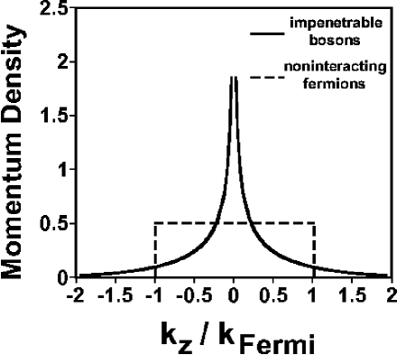
FIG. 2.: Momentum distribution for a system of impenetrable bosons at zero temperature in the thermodynamic limit. Corresponding distribution for an ideal Fermi gas is shown for comparison.

In conclusion, we calculate the one-dimensional scattering amplitude and effective one-dimensional interaction potential for atoms transversally confined by a two-dimensional harmonic potential. We suggest a realization of the Tonks gas – a one-dimensional gas of impenetrable bosons. From the experimental point of view the impenetrable bosons regime corresponds to highly elongated traps (waveguides) at low temperatures ($k_{\rm B}T\ll\hbar\omega_{\perp}$) and at low linear densities ( $\rho a\ll(2\pi)^{-1}(a/a_{\perp})^{2}$, $a>0$). We give an estimate for suitable experimental parameters for alkali atoms confined in waveguides.

We would like to express our appreciation for many useful discussions with Y. Castin, R. Dum, K. Johnson, M. Prentiss, E. Heller, A. Lupu-Sax, M. Naraschewski, V. Lorent, S. P. Smith, C. Herzog, C. A. Tracy, V. E. Korepin, and J. M. Doyle.

M.O. was supported by the National Science Foundation grant for light force dynamics #PHY-93-12572 and by the grant PAST of the French Government. This work was also partially supported by the NSF through a grant for the Institute for Theoretical Atomic and Molecular Physics at Harvard University and the Smithsonian Astrophysical Observatory. Laboratoire Kastler-Brossel is an unité de recherche de l’Ecole Normale Supérieure et de l’Université Pierre et Marie Curie, associée au CNRS.

REFERENCES

- [1] M. H. Anderson, J. R. Ensher, M. R. Matthews, C. E. Wieman, E. A. Cornell, Science, 269, 5221 (1995); K. B. Davis, M.-O. Mewes, M. R. Andrews, N. J. van Druten, D. S. Durfee, D. M. Kurn, W. Ketterle, Phys. Rev. Lett., 75, 3969 (1995); C. C. Bradley, C. A. Sackett, R. G. Hulet, Phys. Rev. Lett., 78, 985 (1997)
- [2] M. A. Ol’shanii, Yu. B. Ovchinnikov, V. S. Letokhov, Optics Communications, 98, 77 (1993); S. Marksteiner, C. M. Savage, P. Zoller, S. L. Rolston, Phys. Rev. A, 50, 2680 (1994); M. J. Renn, D. Montgomery, O. Vdovin, D. Z. Anderson, C. E. Wieman, E. A. Cornell, Phys. Rev. Lett., 75, 3253 (1995); for a review see also J. P. Dowling and J. Gea-Banacloche, Advances in Atomic, Molecular, and Optical Physics, 37, 1 (1996)
- [3] L. V. Hau, J. A. Golovchenko, M. M. Burns, Phys. Rev. Lett., 74, 3138 (1995); J. Schmiedmayer, Applied Physics B, 60, 169 (1995)
- [4] W. Ketterle, and N. J. van Druten, Phys. Rev. A 54, 656 (1996)
- [5] L. Tonks, Phys. Rev., 50, 955 (1936); M. Girardeau, J. Math. Phys., 1, 516 (1960); A. Lenard, J. Math. Phys., 7, 1268 (1966)
- [6] C. N. Yang and C. P. Yang, J. Math. Phys., 10, 1115 (1969)
- [7] V. E. Korepin, N. M. Bogoliubov, and A. G. Izergin, Quantum Inverse Scattering Method and Correlation Functions (Cambridge University Press, Cambridge, 1993)
- [8] E. H. Lieb and W. Liniger, Phys. Rev. 130, 1605 (1963)
- [9] K. Huang, Statistical Mechanics (John Wiley & Sons, New York, 1987)
- [10] For example , , .
- [11] Recall that according to the condition (4) the value of is bounded from below as .
- [12] L. D. Landau and R. M. Lifshitz, Quantum Mechanics: Nonrelativistic Theory, §§132-133 (Oxford, Pergamon, 1965)
- [13] G. M. d’Ariano, A. Montorsi, and M. G. Rasetti (eds.), Integrable Systems in Statistical Mechanics (World Scientific, Singapore, 1985)
- [14] H. G. Vaidya and C. A. Tracy, Phys. Rev. Lett., 42, 3 (1979); a corrected version of the expansions can be found in M. Jimbo, T. Miwa, Y. Mori, and M. Sato, Physica, 1D, 80 (1980)
- [15] J. R. Gardner, R. A. Cline, J. D. Miller, D. J. Heinzen, H. M. J. M. Boesten, B. J. Verhaar, Phys. Rev. Lett., 74, 3764 (1995)
- [16] E. Tiesinga, C. J. Williams, P. S. Julienne, K. M. Jones, P. D. Lett, W. D. Phillips, [NIST J. Res. 101, 505 (1996) ], special issue on BEC, edited by K. Burnett, M. Edwards, and C. Clark