Exact Correlation Amplitude for the S=1/2 Heisenberg Antiferromagnetic Chain

Abstract

The exact amplitude for the asymptotic correlation function in the S=1/2 Heisenberg antiferromagnetic chain is determined:

$$<S^{a}_{0}S^{b}_{r}>\to(-1)^{r}\delta^{ab}(\ln r)^{1/2}/[(2\pi)^{3/2}r].$$

The behaviour of the correlation functions for small xxz anisotropy and the form of finite-size corrections to the correlation function are also analysed.

The asympototic behaviour of the equal-time correlation function in the Heisenberg antiferromagnetic chain has been difficult to determine numerically[1, 2, 3, 4, 5] because of the presence of a marginally irrelevant operator. This leads[6, 7] to a logarithmic factor of $\sqrt{\ln r}$ and also to finite size effects which only vanish as $1/\ln L$ where L is the system size. This marginal operator leads to logarithmic corrections, sometimes multiplicative and sometimes additive, to most long distance, low energy properties of the model. In particular recent experiments on Sr₂CuO₃ found evidence for the predicted [8] logarithmic additive correction to the susceptibility [9].

On the other hand, logarithmic corrections are absent for the xxz model, with Hamiltonian:

$$H=\sum_{i}[(S^{x}_{i}S^{x}_{i+1}+S^{y}_{i}S^{y}_{i+1}+\gamma S^{z}_{i}S^{z}_{i+1}],$$ (1)

for $\gamma\neq 1$. The model exhibits critical behaviour for $-1\leq\gamma\leq 1$, with asympotic correlation functions:

$$G^{x}(r)\equiv<S^{x}_{0}S^{x}_{r}> \to (-1)^{r}A_{x}r^{-\eta}$$ (2)

$$G^{z}(r)\equiv<S^{z}_{0}S^{z}_{r}> \to (-1)^{r}A_{z}r^{-1/\eta},$$ (3)

with

$$\eta=1-[\cos^{-1}\gamma]/\pi\ \ (0\leq\eta\leq 1).$$ (4)

What appears to be an exact formula for the amplitude $A_{x}(\gamma)$ was recently conjectured [10]:

$$A_{x}(\gamma)={(1+\xi)^{2}\over 8}\left[{\Gamma({\xi\over 2})\over 2\sqrt{\pi}\Gamma\left({1\over 2}+{\xi\over 2}\right)}\right]^{\eta}\times\exp\left\{-\int_{0}^{\infty}{dt\over t}\left({\sinh(\eta t)\over\sinh(t)\cosh[(1-\eta)t]}-\eta e^{-2t}\right)\right\}.$$ (5)

Here:

$$\xi\equiv{\eta\over 1-\eta}.$$ (6)

The main purpose of the present report is to determine the exact amplitude in the logarithmic, xxx case, $\gamma=1$, giving the result in the abstract. To do so it will be neccessary to consider the form of these correlation functions for $\gamma$ only slightly less than 1 where a crossover from logarithmic to non-logarithimic behaviour occurs. The other amplitude, $A_{z}$, is not known in general. We will show that:

$$\lim_{\gamma\to 1^{-}}A_{z}/A_{x}=4.$$ (7)

The order of limits here is crucial; right at $\gamma=1$ the amplitudes of the (logarithmic) correlation functions $G^{x}$ and $G^{z}$ are equal. We also discuss the form of finite-size corrections for the correlation function on a ring of length L with periodic boundary conditions, $G(r,L)$.

The subsequent calculations are based on the continuum limit bosonized approximation to the xxz model. We follow the notation of [6]. The Hamiltonian density may be written:

$${\cal H}={\cal H}_{0}-(8\pi^{2}/\sqrt{3})[g^{x}(J_{L}^{x}J_{R}^{x}+J_{L}^{y}J_{R}^{y})+g^{z}(J_{L}^{z}J_{R}^{z})].$$ (8)

Here ${\cal H}_{0}$ is the Hamiltonian density for a free boson, of compactification radius $R=1/\sqrt{2\pi}$, or equivalently, the SU(2) level 1 Wess-Zumino-Witten (WZW) non-linear $\sigma$ model. $\vec{J}_{L,R}$ are the left and right moving currents. (We set the spin-wave velocity equal to 1.) For the isotropic model, with $\gamma=1$, $g^{x}=g^{z}=g$ is of O(1). The rather cumbersome normalization in Eq. (8) is dictated by the convention that the operator multiplying $g$ in the isotropic case have a correlation function with unit amplitude. For the xxz model with $\gamma$ close to 1,

$$g^{z}-g^{x}\propto 1-\gamma.$$ (9)

These coupling constants obey the Kosterlitz-Thouless renormalization group (RG) equations:

$$\beta_{z}\equiv dg_{z}/d\ln L = -(4\pi/\sqrt{3})g_{x}^{2},$$ (10)

$$\beta_{x}\equiv dg_{x}/d\ln L = -(4\pi/\sqrt{3})g_{x}g_{z}.$$ (11)

The RG trajectories are sketched in Fig. 1. $g_{z}^{2}(L)-g_{x}^{2}(L)$ is an RG invariant along the flow. For $g_{z}>|g_{x}|$, the flow is to a fixed line, the positive $g_{z}$ axis. $g_{z}^{2}(L)-g_{x}^{2}(L)=g_{z}^{2}(\infty)$ along these trajectories. Using the abelian bosonization formula $J^{z}_{L}=-(1/\sqrt{8\pi})(\partial_{0}+\partial_{1})\phi$, we find that, at the fixed point, the effective Lagrangian is:

$${\cal L}=(1/2)(\partial_{\mu}\phi)^{2}[1-(2\pi g_{z}(\infty)/\sqrt{3}].$$ (12)

The staggered part of the local spin operators may be written in non-abelian bosonization notation as:

$$\vec{S}_{i}\propto(-1)^{i}\hbox{tr}g\vec{\sigma},$$ (13)

where $g$ is the two dimensional unitary matrix field of the WZW model. In terms of abelian bosonization:

$$S^{z}_{i} \propto (-1)^{i}\sin(\phi/R)$$ (14)

$$S^{x}_{i} \propto (-1)^{i}\cos(2\pi R\tilde{\phi}),$$ (15)

where $\tilde{\phi}$ denotes the dual field and $R=1/\sqrt{2\pi}$. From Eqs. (12) and (15) we can determine the correlation exponents of Eq. (3) with:

$$\eta=1-2\pi g_{z}(\infty)/\sqrt{3}.$$ (16)

Note that, using Eq. (4), determined from the Bethe ansatz solution, the value of $g_{z}(\infty)$ is determined exactly. The scaling dimensions of the staggered spin operators tr$g\sigma^{x}$ and tr$g\sigma^{z}$ are given by $\eta/2$ and $1/2\eta$ respectively. To study the logarithmic behaviour, we will also need the anomalous dimensions for small non-zero $g_{i}$, along the RG trajectories. These can be determined from the 3-point Green’s functions $<\hbox{tr}g\sigma^{a}J_{L}^{b}J_{R}^{b}\hbox{tr}g\sigma^{a}>$ as in [6]. Using the fact that the operator product expansion gives:

$$J_{L}^{b}(z)J_{R}^{b}(\bar{z})g(z^{\prime},\bar{z}^{\prime})\to{(1/4)\sigma^{b}g\sigma^{b}\over|2\pi(z-z^{\prime})|^{2}}+\ldots,$$ (17)

we conclude that:

$$<\hbox{tr}g\sigma^{a}J_{L}^{b}J_{R}^{b}\hbox{tr}g\sigma^{a}>\propto\hbox{tr}(\sigma^{a}\sigma^{b}\sigma^{a}\sigma^{b})=4\delta^{ab}-2.$$ (18)

Thus, to linear order, the conclusion is:

$$\gamma_{x} = 1/2-(\pi/\sqrt{3})g_{z},$$ (19)

$$\gamma_{z} = 1/2+(\pi/\sqrt{3})(g_{z}-2g_{x}).$$ (20)

FIG. 1.: The Kosterlitz-Thouless RG flows of Eq. (11).

In discussing the asympototic correlation functions, using bosonization, it is convenient to introduce uniform and staggered terms:

$$G^{i}(r)\to G^{i}_{u}(r)+(-1)^{r}G^{i}_{s}(r),$$ (21)

where $G^{i}_{u}$ and $G^{i}_{s}$ vary slowly on the scale of a lattice spacing. These two terms correspond to different Green’s functions in the continuum limit field theory. In this paper we only discuss the staggered term.

The staggered correlation functions (for an infinite spin chain) obey the RG equations:

$$[\partial/\partial\ln r+\sum_{j}\beta_{j}(\vec{g})\partial/\partial g_{j}+2\gamma_{i}(\vec{g})]G_{s}^{i}(r,\vec{g})=0.$$ (22)

Here $\vec{g}\equiv(g_{z},g_{x})$. This follows from the fact that a rescaling of the length is equivalent to a change in the values of the effective coupling constants together with a rescaling of the fields with exponents $\gamma_{i}$. The solution of Eq. (22) is:

$$G_{s}^{i}(r,\vec{g}^{0})=\exp\{-2\int_{r_{0}}^{r}d\ln r^{\prime}\gamma_{i}[\vec{g}(r^{\prime})]\}F^{i}[\vec{g}(r)],$$ (23)

where the $F^{i}$ are arbitrary functions of $\vec{g}(r)$, the solution of the RG equations,

$$dg_{i}/d\ln r=\beta_{i}(\vec{g}).$$ (24)

Here $\vec{g}^{0}\equiv\vec{g}(r_{0})$, denotes the value of the “bare” couplings at some reference “ultraviolet cut off” scale $r_{0}$ of order a lattice spacing. Since, for large r, $g_{x}(r)<<1$, we may expand the functions $F_{i}[\vec{g}(r)]$ perturbatively in $g_{x}(r)$. Exactly this procedure is used to analyse deep inelastic scattering data in quantum chromodynamics. It is known as “renormalization group improved perturbation theory”. To lowest order these functions are just constants. Integrating the RG equations for the effective coupling constants, Eq. (11) we obtain:

$$g_{x}(r) = {\sqrt{3}\epsilon\over 4\pi}\hbox{cosech}(\epsilon\ln r)$$ (25)

$$g_{z}(r) = {\sqrt{3}\epsilon\over 4\pi}\coth(\epsilon\ln r),$$ (26)

where we have defined:

$$\epsilon\equiv 2(1-\eta)=4\pi g_{z}(\infty)/\sqrt{3}.$$ (27)

Now performing the integration over $\gamma_{i}(\ln r)$ in Eq. (23), we obtain:

$$G_{s}^{x}(r) \to {A_{x}\over r^{1-\epsilon/2}}(1-r^{-2\epsilon})^{1/2}$$ (28)

$$G_{s}^{z}(r) \to {A_{z}\over r^{1+\epsilon/2}}{(1-r^{-\epsilon})^{1/2}\over(1+r^{-\epsilon})^{3/2}}.$$ (29)

Note that we have defined the normalization constants so that the asympotic large-r behaviour is as in Eq. (3). Also note that, for $\epsilon<<1$, both correlation functions exhibit logarithimic behaviour over an intermediate range of r, $1<<\ln r<<1/\epsilon$. In this range of r, we obtain:

$$G_{s}^{x} \approx \sqrt{2\epsilon}A_{x}{(\ln r)^{1/2}\over r}$$ (30)

$$G_{s}^{z}(r) \approx {\sqrt{\epsilon}A_{z}\over 2^{3/2}}{(\ln r)^{1/2}\over r}.$$ (31)

Now consider taking the limit $\epsilon\to 0$, corresponding to the isotropic Heisenberg antiferromagnet. We see that in order for the correlation functions to remain finite at fixed r as $\epsilon\to 0$ we must have $A_{x}\propto 1/\sqrt{\epsilon}$. Furthermore, in order to obtain the isotropic result, $G_{s}^{x}(r)=G_{s}^{z}(r)$, we must have $A_{z}/A_{x}\to 4$, as $\epsilon\to 0$. Thus for small but finite $\epsilon$, $G_{s}^{x}(r)\approx G_{s}^{z}(r)$ in the intermediate range of r, but at very large r they exhibit slightly different exponents and amplitudes differing by a factor of 4.

The exact amplitude, $A_{x}(\eta)$ of Eq. (5) can be evaluated in closed form in the limit $\eta\to 1$, $\epsilon\to 0$. In this limit we may approximate $\sinh\eta t/\sinh t\approx e^{-\epsilon t/2}$ in the first term of the integrand and $\eta\approx 1$ in the second term. The integral can then be done exactly, giving:

$$A_{x}\to{1\over 4(\epsilon)^{1/2}\pi^{3/2}}.$$ (32)

This diverges as $1/\sqrt{\epsilon}$, as expected. Thus we conclude, in the isotropic case:

$$G_{s}^{z}(r)=G_{s}^{x}(r)\to{1\over(2\pi)^{3/2}}{(\ln r)^{1/2}\over r}.$$ (33)

The asymptotic form of the Fourier transform for $k\approx\pi$ is thus given by:

$$G(k)\equiv\sum_{r=-\infty}^{\infty}G(r)e^{ikr}\to{4\over 3(2\pi)^{3/2}}|\ln|k-\pi||^{3/2}.$$ (34)

Note that the effect of the $(\ln r)^{1/2}$ factor is to change the power of $|\ln|k-\pi||$ from 1 to 3/2. If such a weak singularity could be observed, this formula might be useful to check the normalization in neutron scattering experiments. It follows from the above analysis that, for small xxz anisotropy, this isotropic formula remains valid down to exponentially small values of $k-\pi$, making the log singularity of Eq. (34) observable.

Several efforts have been made to check the field theory prediction of logarithmic behaviour numerically [1, 2, 3, 4, 5]. Hallberg et al. [4] obtained the above asympototic behaviour but with an amplitude of .06789 in place of the exact result $(2\pi)^{-3/2}=.06349364\ldots$. This result was obtained from density matrix renormalization group calculations on rings of up to 70 sites using finite-size extrapolation. Koma and Mitzukoshi [5] also obtained the above form with an amplitude of .065. [Alternatively, if they let the power of the logarithm be a free parameter they obtained a slightly better fit with a power of .47 instead of 1/2 and an amplitude of .071.] This was obtained using exact diagonalization results for $L\leq 30$ and zero temperature quantum Monte Carlo for $32\leq L\leq 80$. The agreement is remarkably good considering the severe difficulties of the extrapolation due to the logarithmic nature of the corrections. In the remainder of this report we consider the nature of the corrections to this formula, for the Heisenberg antiferromagnet.

Let us begin with $G_{s}(r)$ for an infinite system. The integral in the exponent in Eq. (23) can be rewritten as:

$$\int_{g_{0}}^{g(r)}[\gamma(g)/\beta(g)]dg = (1/2)\ln(r/r_{0})+\int_{g_{0}}^{g(r)}\left[{1\over 4g}+\sum_{n=0}^{\infty}a_{n}g^{n}\right]$$ (35)

$$= (1/2)\ln(r/r_{0})+(1/4)\ln[g(r)/g_{0}]+\sum_{n=0}^{\infty}{a_{n}\over n+1}[g(r)^{n+1}-g_{0}^{n+1}].$$ (36)

Here the $a_{n}$ terms arise from the higher order terms in the perturbative expansions of $\beta(g)$ and $\gamma(g)$. Noting that all terms involving $g_{0}$ are just constants, and also Taylor expanding the function $F[g(r)]$ in Eq. (23), we may finally write:

$$G_{s}(r)\to{1\over r\sqrt{g(r)}}\sum_{n=0}^{\infty}b_{n}g^{n}(r),$$ (37)

in terms of some combined coefficients, $b_{n}$. Including the cubic term in the $\beta$-function for the isotropic case[11]:

$$dg/d\ln r=-(4\pi/\sqrt{3})g^{2}-(1/2)(4\pi/\sqrt{3})^{2}g^{3}.$$ (38)

Integrating gives:

$${1\over g(r)}-{1\over g_{0}}=(4\pi/\sqrt{3})\{\ln(r/r_{0})+(1/2)\ln[\ln(r/r_{0})]\}+O(1).$$ (39)

Thus, we may write:

$$G_{s}(r)={1\over(2\pi)^{3/2}}{\{\ln(r/r_{0})+(1/2)\ln[\ln(r/r_{0})]\}^{1/2}\over r}[1+O(1/\ln r)].$$ (40)

We may absorb the leading correction into a constant term inside the square root:

$$G_{s}(r)={1\over(2\pi)^{3/2}}{\{\ln(Cr/r_{0})+(1/2)\ln[\ln(r/r_{0})]\}^{1/2}\over r}\{1+O[1/(\ln r)^{2}]\}.$$ (41)

From Eq. (39), $C$ has the form:

$$C=e^{\sqrt{3}/4\pi g_{0}+O(1)}.$$ (42)

The O(1) term in the exponent in Eq. (42) could be computed. It requires calculation of the anomalous dimension $\gamma(g)$ to $O(g^{2})$ and of the function $F$ to O(g). This term was ignored in [4] leading to an inaccurate determination of $g_{0}$.

Let us now consider the Green’s function on a ring of length L, $G_{s}(r,r/L,g)$. The RG equation, Eq. (22), is still obeyed. The derivative in this equation may be taken either with respect to r or L with the ration r/L held fixed. This follows because a rescaling of both length scales is equivalent to a coupling constant redefinition. Using an L-derivative, the solution is now:

$$G_{s}(r,L,g^{0})=\exp\{-2\int_{r_{0}}^{L}d\ln r^{\prime}\gamma[g(r^{\prime})]\}F[g(L),r/L],$$ (43)

The exponential factor is independent of $r$. The function $F[g(L),r/L]$ may be expanded perturbatively in $g(L)$ for large $L$:

$$F[g(L),r/L]=\sum_{n=0}^{\infty}g(L)^{n}F_{n}(r/L).$$ (44)

The various functions $F_{n}(r/L)$ can be calculated by doing perturbation theory in the system with finite length. They should all obey the periodicity requirement:

$$F_{n}[r/L]=F_{n}[(L-r)/L].$$ (45)

If we take the asymptotic limit $r/L\to 0$, we should recover the infinite L result of Eq. (41). The zeroth order term, $F_{0}(r/L)$ is obtained by ignoring the marginal interaction altogether and simply calculating:

$$<\hbox{tr}(\vec{\sigma}g)(r)\cdot\hbox{tr}(\vec{\sigma}g)(0)>_{L}$$ (46)

in the conformally invariant WZW model, on a circle of length L. The correlation function on the circle (i.e. the cylinder in the space-time picture) is simply obtained by a conformal transformation and is given by:

$$<\hbox{tr}(\vec{\sigma}g)(r)\cdot\hbox{tr}(\vec{\sigma}g)(0)>_{L}\propto{1\over L\sin(\pi r/L)}.$$ (47)

Thus we may write:

$$G_{s}(r,L)\to{1\over(2\pi)^{3/2}}{\{\ln(L/r_{0})+(1/2)\ln[\ln(L/r_{0})]\}^{1/2}\over(L/\pi)\sin(\pi r/L)}\left[1+{1\over\ln(L/r_{0})}\tilde{F}_{1}(r/L)+\ldots\right],$$ (48)

for some other scaling function, $\tilde{F}_{1}$. Alternatively, solving the RG equation with an r-derivative, we obtaine this result with L replaced by r inside all logarithms and a different scaling function $F_{1}^{\prime}(r/L)$. [Note that, taking $r>>r_{0}$ with $r/L$ held fixed, the difference between $\sqrt{\ln(r/r_{0})}$ and $\sqrt{\ln(L/r_{0})}$ is suppressed by a factor of $1/\ln(r/r_{0})$.]

For the general xxz model the leading order finite-size scaling result is again obtained by the simple replacement:

$$r\to(L/\pi)\sin(\pi r/L).$$ (49)

In particular, for $G_{s}^{x}$ in the xx model ($\gamma=0$) we obtain:

$$G_{s}^{x}\propto[\sin(\pi r/L)]^{-1/2}.$$ (50)

The corrections are down by powers of 1/r rather than only logarithms.

The efforts to fit numerical results on correlation functions in S=1/2 antiferromagets to a finite-size scaling form have a rather curious history. The case of $G_{s}^{x}$ for the xx model was considered in [1]. Rather than using the result predicted by conformal invariance the authors adopted a phenomenological expression, with free parameters adjusted to obtain good data collapse, corresponding to the replacement:

$$\left({\pi x\over\sin\pi x}\right)^{1/2}\to 1+.28822\sinh^{2}(1.673x),$$ (51)

for $x\equiv r/L$. This leads to a correlation function not obeying the periodicity condition:

$$G(r,L)=G(L-r,L).$$ (52)

Thus, the data fitting was only done for $0<x<1/2$. Over this range, these two functions actually agree to within about .05% as indicated in Figure 2. This indicates that the conformal field theory (CFT) prediction is extremely accurate for the xx model. It was proposed in [1] that, in the general xxz model, one should use the form:

$$[1+.28822\sinh^{2}(1.673x)]^{2\eta},$$ (53)

for $G_{s}^{x}$. This is essentially the correct CFT prediction, due to the numerical agreement noted above. However, in [4] the exponent in Eq. (53) was taken to be a free parameter. For the Heisenberg model a best fit was obtained with the exponent $1.805$ rather than the correct value of 2. Thus the scaling form used differed slightly from the one predicted by CFT as shown in Fig. 3. The maximum disagreement, at $x=.5$, is about 4%.

Koma and Mizukoshi used the scaling function

$$G_{s}(r,L)\to{A\{\ln[(L/\pi r_{0})\sin(\pi r/L)]\}^{1/2}\over(L/\pi)\sin(\pi r/L)},$$ (54)

obtaining a best fit for $A\approx.065$ (close to $(2\pi)^{-3/2}\approx.0635$). The agreement between this formula and their numerical data is better than 1.26% for $1\leq r\leq L/2$ and $4\leq L\leq 80$. Taylor expanding in $1/\ln(L/r_{0})$, we see that this expression is consistent with Eq. (48) for a particular choice of the function $\tilde{F}_{1}$, up to the small discrepancy in the amplitude. Eq. (54) has the great advantage of simultaneously having the correct periodicity property and the correct behaviour in the limit $L\to\infty$. However, such an expression can only arise from Eq. (43) by summing an infinite number of terms in Eq. (44) [and ignoring the $\ln[\ln(L/r_{0})]$ terms in $g(L)$].

We expect that the somewhat larger discrepancy with CFT for the Heisenberg model than for the xx model can be accounted for by the log corrections. The range of r used in the numerical work of Hallberg et al. [4] for which fairly good data collapse was obtained was only $10<r<30$. In this range we might expect the factor $1/\ln(r/r_{0})$ in Eq. (48) (written with r replaced by L inside the logarithms) to be fairly constant. Thus the $F_{1}^{\prime}$ term acts essentially as a small correction to the scaling function, $\pi x/\sin(\pi x)$. (A related observation was made in [5].) It is feasible to push this renormalization group improved perturbation theory to one higher order and calculate $\tilde{F}_{1}(r/L)$ in Eq. (48). This involves using the known result for the $\beta$-function to $O(g^{3})$, calculating the anomalous dimension to $O(g^{2})$ and calculating the Green’s function on a finite strip to $O(g)$. We expect that this could give better agreement with the numerical results and could, in particular, reduce the small discrepancy between the exact amplitude and the results of [4] and [5].

FIG. 2.: Comparison of the 2 different scaling functions for the xx model.

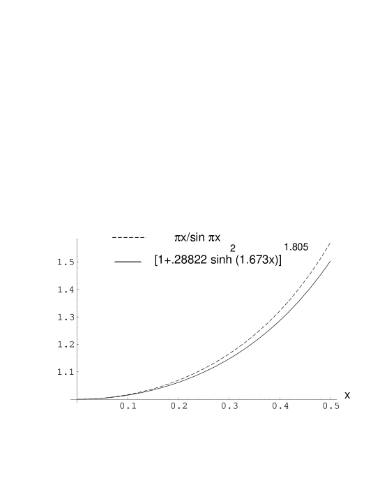
FIG. 3.: Comparison of the 2 different scaling functions for the xxx model.

I would like to thank M. Oshikawa for very helpful discussions and S. Lukyanov for informing me of his work. After this paper was completed I encountered the recent preprint [12] which has some overlap with the results derived here. This research was supported by NSERC of Canada.

REFERENCES

[1] K. Kubo, T.A. Kaplan and J. Borysowicz, Phys. Rev. B38, 11550
(1988).
[4] K. Hallberg, P. Horsch and G. Martinez, Phys. Rev. B52,
R719 (1995).
[5]T. Koma and N. Mizukoshi, J. Stat. Phys. 83, 661 (1996).
[6] I. Affleck, D. Gepner, H.J. Schulz and T. Ziman, J. Phys. A22,
511 (1989). For a review see I. Affleck, Fields, Strings and Critical Phenomena
[ed. E. Brézin and J. Zinn-Justin, North-Holland, Amsterdam, 1989]; 511.
[7] R.R. Singh, M.E. Fisher and R. Shankar, Phys. Rev. B39, 2562
(1989).
[8] S. Eggert, I. Affleck and M. Takahashi, Phys. Rev. Lett. 73, 332
(1994).
[9] T. Ami et al., Phys. Rev. B51, 5994 (1995); S. Eggert, Phys. Rev.
B53, 5116 (1996); N. Motoyama et al., Phys. Rev. Lett. 76, 3212 (1996).
[10]S. Lukyanov and A. Zamalodchikov, Nucl. Phys. B493, 571
(1997).