Ginzburg-Landau Theory for Impure Superfluid ³He

Abstract

Liquid ³He at low temperatures is an ideal substance to study because of its natural purity. The superfluid state, which appears at temperatures below 3 mK, has many unusual and exciting properties. These have extensively been studied experimentally, and the results are in many cases well understood theoretically using quasiclassical approximation. In this work we study the case that liquid ³He is inside of aerogel. Aerogel is a very porous substance, where 98% of the volume can be empty. The purpose is to understand how the properties of the superfluid are modified when the quasiparticles are scattered from an impurity, such as aerogel. We study extensively the homogeneous scattering model. From it we derive the Ginzburg-Landau theory of impure superfluid ³He. We give expressions for measurable quantities and compare them with experiments. We consider random anisotropy and its effect on the NMR properties. More sophisticated scattering models are briefly discussed.

1 Introduction

Liquid ³He at low temperatures is the purest substance in Nature because usual impurities simply will fall down by gravity. This is one of the reasons why liquid ³He, in spite of its strong particle-particle interactions, is one of the best understood condensed matter systems ([3Hereview]). Especially the superfluid state, which occurs at temperatures below 3 mK, shows many complicated but still well understood phenomena. But the purity can also be a limitation because often important physical effects exist only because of impurities. For example, except of a few marginal cases, all pure elemental superconductors are of type I. That is, type II superconductivity, where magnetic field penetrates into the superconductor as quantized flux lines, exist because of impurities which radically change the properties of pure elements.

One type of impurity is formed by the surfaces of the container that hold the liquid. There has been several studies of liquid ³He in different confined geometries, for example between parallel plates or in packed powders (for example, [TholenParpia]). In these cases the effect on ³He arises from walls, i.e. from 2-dimensional interfaces between ³He and a foreign object. It is very difficult to support zero-dimensional (point-like) impurities in liquid ³He. However, there is the intermediate case of one-dimensional impurities. This type of impurity can approximately be realized by silica aerogels. These are very porous materials where, for example, 98% of the volume is empty. Several recent experiments investigate ³He in aerogel ([Porto, Matsumoto, Sprague1], 1996). It is found that, similar to the bulk liquid, ³He in aerogel goes to the superfluid state, but both the superfluid transition temperature $T_{\rm c}$ and the amplitude of the superfluid state are reduced compared to the pure case. The measured suppression of $T_{\rm c}$ is shown in Fig. 1.

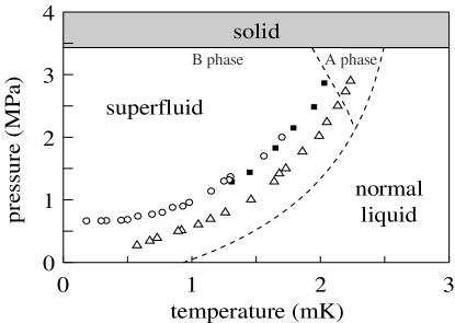
Figure 1: The measured superfluid transition points of ³He in aerogel: Porto and Parpia (1995, △), Sprague et al. (1995,  ), and Matsumoto et al. (1997, $\circ$). The dashed lines denote the normal-superfluid and the A-B transition lines in pure ³He. The A and B phases also refer to pure ³He.

In this article we present some theoretical ideas concerning ³He in aerogel. We first describe the structure of aerogel (Section 2). The main effect of aerogel on superfluid ³He arises from scattering of the quasiparticles of ³He from the aerogel impurity. This effect can be calculated to a good approximation using the quasiclassical theory. The general assumptions of quasiclassical scattering models are discussed in Section 3. In Section 4 we study a model where the scattering is considered as homogeneously distributed. We will limit to temperatures in the neighborhood of the transition temperature $T_{\rm c}$, and derive the Ginzburg-Landau theory. We calculate measurable quantities and compare them with experiments. We find that more sophisticated scattering models are needed in order to explain the measurements quantitatively (Section 5). The anisotropy of the scattering is considered in Section 6. There we study a random field model using similar arguments as presented by Imry and Ma (1975), and find that the NMR properties crucially depend on the anisotropy.

2 Aerogel

A nice introduction to aerogels is given by Fricke (1988). The fabrication uses a gelation process in the liquid phase. A variety of aerogel materials are possible, but the present ones are of silica, (SiO₂)_n. In order to get aerogel it is crucial to preserve the gel structure when the solvent is removed. This is not trivial because the surface tension of the liquid–gas interface would make the gel to collapse in straightforward drying. Fortunately, it is possible to go continuously from the liquid to the gas phase. For that one has to move along such a path that goes around the critical point ($T_{0}$, $p_{0}$) in the temperature–pressure plane. In order to avoid too high temperatures and pressures, methanol (512 K, 8 MPa) is preferred to water (647 K, 22 MPa) as a solvent.

The experiments with superfluid ³He use samples where the aerogel fills only 2% of the total volume, $V=0.02$. The surface to volume ratio is determined by measurements with ⁴He, and they give $A=260000\ {\rm cm}^{-1}$ ([KMC]). Based on these numbers alone, we can make some estimations of the dimensions in aerogel. If we assume that the structure is a lattice of one-dimensional strands, we calculate the strand diameter ${4V/A}=3$ nm and the distance between neighboring strands ${\sqrt{4\pi V}/A}=20$ nm. The mean free path for straight line trajectories is estimated as $\ell={4/A}=150$ nm. Although this picture is certainly very idealized, the numbers are not very different from the ones obtained by other means such as transmission electron microscopy or low-angle x-ray scattering. The distance between strands certainly has large variation because of fluctuations in the local aerogel density.

The next step in understanding superfluid ³He in aerogel is to study the characteristic lengths of ³He. The smallest scale is the average distance between neighboring ³He atoms. This is on the same order of magnitude as the Fermi wave length $\lambda_{\rm f}=2\pi/k_{\rm f}\approx 0.7$ nm. This is somewhat smaller than the diameter of the strands. A much larger scale is the coherence length $\xi_{0}={\hbar v_{\rm f}/2\pi k_{\rm B}T_{\rm c0}}$. Here $T_{\rm c0}$ is the superfluid transition temperature in bulk ³He and $v_{\rm f}$ is the Fermi velocity. As a function of pressure, $\xi_{0}$ decreases monotonically from 77 nm (zero pressure) to 16 nm (3.4 MPa, the solidification pressure). The coherence length is on the same order as the average strand spacing, but taking into account fluctuations in strand density, we can well expect voids of size larger than $\xi_{0}$. Finally, the mean free path of quasiparticles in pure ³He is $1\ \mu$m or more at the temperatures we are interested in ($T<3$ mK). Thus the scattering from strands is the dominant factor that limits the mean free path in aerogel.

3 Quasiclassical Scattering Models

Before going into the details of different scattering models, it is useful to study the general assumptions. Large part of the ideas presented here are given in a more mathematical form by Buchholtz and Rainer (1979). The following is applicable to both metals and ³He at low temperatures. Here a “particle” refers to an electron in the former case and to a ³He atom in the latter. “Superfluidity” denotes both the superconductivity of metals and the superfluidity of ³He. The many-body hamiltonian of the system can be written as

$$H=H_{\rm pure}+\sum_{j}V_{j}\ .$$ (1)

Here $H_{\rm pure}$ contains the kinetic energies of the particles and interactions between them, and also interaction with the periodic crystal lattice in the case of metals. It may also contain the interaction with external magnetic field, for example. The latter term is the impurity potential. In the case of metals, a common source for it is that some atoms of the lattice are of different type than the others. In the case of ³He, such a term is introduced by the aerogel. Quite generally, the total impurity potential $V$ can be written as a sum so that each term $V_{j}$ is nonzero only in some small region of space. These regions are referred to as “scattering centers”.

The general quasiclassical theory for $H_{\rm pure}$ is discussed extensively by Serene and Rainer (1983), and also elsewhere in this book. The validity of this theory for the superfluid state relies on the assumption $\lambda_{\rm f}\ll\xi_{0}$, which is well satisfied in ³He and in most superconductors. The result is that instead of strongly interacting particles, the system is better understood in terms of quasiparticles. The quasiparticles propagate through the medium similar to classical particles. The interactions between the quasiparticles are weak, and can be neglected in many cases, which would not be the case for particles. Such quasiclassical description is valid for properties that are dominated by processes taking place near the Fermi surface in the momentum space. This includes virtually all phenomena in the superfluid state.

Let us consider adding the impurity effects to the quasiclassical theory. We will not set a limitation to the magnitude of the impurity potential i.e. it can be large, on the order of the Fermi energy $E_{\rm f}$. The crucial assumption is that this large potential occurs only in a limited volume of the total space. This means that the quasiparticle description is still valid in most of the space. The average distance a quasiparticle can travel between it collides with scattering centers defines a mean free path $\ell$. In order to use the quasiparticle picture, $\ell$ has to be large in comparison to the Fermi wave length $\lambda_{\rm f}$. In addition, we neglect coherent scattering from two or more scattering centers. This is justified to leading order in $\lambda_{\rm f}/\ell$ as long as the locations of the scattering centers can be considered random on the scale of $\lambda_{\rm f}$. In other words, the interference can be neglected in an ensemble average if for each scattering center $j$ we have a distribution function $n_{j}({\bf r})$ ($\int d^{3}r\,n_{j}({\bf r})=1$) that is smooth on the scale of $\lambda_{\rm f}$. Note that $n_{j}({\bf r})$ can still be a good approximation to the delta function when looked at on the scale of $\xi_{0}$. In the case that all scattering centers are identical, it is sufficient to specify only one distribution $n({\bf r})$, which is normalized to the total number $N$ of scattering centers: $\int d^{3}r\,n({\bf r})=N$

In a small neighborhood of a scattering center, the state of the system can be strongly different from the bulk. For example, liquid ³He may be in a solid-like state because of the van der Waals interaction with an impurity. In order to allow such changes, the treatment within a scattering center must be fully quantum mechanical. However, such a calculation is not possible in practice because even the wave function of a quasiparticle is not known in any detail. Therefore, one has to introduce the properties of a scattering center by some phenomenological parameters. A sufficient description is to know the scattering $T$ matrix or, in case of an isotropic scattering center, the scattering phase shifts $\delta_{l}$. It is important to notice that these are parameters that appear in the normal state, and they can in principle be measured without need to go into the superfluid state.

The discussion above was limited to the neighborhood of the Fermi surface, where the quasiparticle picture is valid. Because of their strong potential, the impurities also have an effect outside of this range. As a consequence the pairing interaction, for example, is modified by the impurities. However, this effect is of short range because of the relatively high energy. Therefore we can neglect such effects relying on the assumption that the volume fraction of the scattering centers is small. Similar argument gives that the Landau Fermi-liquid parameters ($F_{i}^{\rm s}$, $F_{i}^{\rm s}$), as well as the density ($\rho$) and the dipole-dipole interaction constant ($g_{\rm d}$) in ³He are unchanged.

The size of a scattering center has to be small compared to the length scale one is interested to study. In the superfluid state this scale is typically set by the coherence length $\xi_{0}$. Thus a scattering center has to be small compared to $\xi_{0}$, although it can be large compared to $\lambda_{\rm f}$. It should be noted that the size of the scattering center does not limit the size of the impurity. In order to consider a macroscopic body, we represent its surface by a set of scattering centers. This is possible because for all practical bodies, the height-height correlations $\langle\zeta({\bf r})\zeta({\bf r}+\delta{\bf r})\rangle$ of the surface have a distribution that is much wider that $\lambda_{\rm f}$ when the separation $\delta r$ is on the order of $\xi_{0}$. Thus the scattering becomes incoherent on this scale, and therefore can be represented by different scattering centers. Assuming that the particles cannot penetrate into the body, the volume of the body should be excluded from the calculation. For example, we estimate the volume of scattering centers in aerogel as the volume of few atomic layers on the strands ($\approx\lambda_{\rm f}A$) rather than the volume of the strands themselves ($V$). (It happens, however, that both quantities are on the same order of magnitude in this case).

Let us comment the effect of the pairing state. Superfluidity arises because part of the quasiparticles are weakly bound to pairs. The momenta of the quasiparticles in a pair can be denoted by ${\bf p}$ and $-{\bf p}$ because the total momentum of the pair is small. The dependence of the pair wave function on the direction $\hat{\bf p}={\bf p}/p$ can be described using spherical harmonic functions and classified as $s$, $p$, $d$, etc. states. In most superconducting metals the Cooper pairs form dominantly in an $s$-wave state. In ³He the pairs form in a $p$-wave state, and there is increasing evidence that $d$ waves are dominant in high-$T_{\rm c}$ cuprate superconductors. The amplitude of the superfluid state and the transition temperature can be calculated for these cases as a function of impurity scattering, as will be discussed in more detail later. In the quasiclassical approximation one finds that the impurities have no effect on a homogeneous $s$-wave superfluid. For other waves the superfluidity is suppressed by impurity, and it disappears when the mean free path is reduced to $\sim\xi_{0}$. The interpretation is that scattering changes the momenta of the quasiparticles, but this has no effect in the s-wave case because the wave function is independent of the momentum direction. For other waves the sign of the wave function changes for certain scattering angles, which leads to destructive interference. There is an effect for $s$ waves, too, if the superfluid state is inhomogeneous. Here the scattering makes the quasiparticles more localized, and therefore they see more the same order parameter. This effect makes the superconductor less sensitive to magnetic field, i.e. causes the change from type I to type II superconductivity, as mentioned in the introduction.

All the discussion above has been in weak-coupling limit. This means neglecting all corrections that are proportional to the small ratio $\lambda_{\rm f}/\xi_{0}$. This approximation is clearly inadequate for some properties of ³He. For example, it gives that the B phase is always more stable than the A phase, contrary to the phase diagram in Fig. 1. There are some calculations of strong coupling corrections in the pure ³He ([SRrev]). It seems very difficult to take these corrections into account in the impure case, and therefore we do not consider them here.

4 Homogeneous Scattering Model

We do not know the precise distribution $n({\bf r})$ of scattering centers in aerogel. Therefore we have to take a model for $n({\bf r})$. The simplest possible one is the homogeneous scattering model (HSM). There one assumes that $n({\bf r})=n$ is a constant. In other words, the probability for a quasiparticle to be scattered is the same at all locations ${\bf r}$. This same approximation is commonly used to study impurities in superconductors ([Gorkov, AG]).

The mean free path in the HSM is given by $\ell=(n\sigma)^{-1}$. Here $\sigma$ is the scattering cross section of a scattering center. We additionally assume that the medium is isotropic, i.e. $\ell$ is independent of the direction of quasiparticle momentum. We also assume that the scattering is nonmagnetic. This means that the scattering probability is the same for both directions of the spin, and the spin is not changed in the scattering.

A convenient property of the isotropic HSM is that both the Ginzburg-Landau (GL) theory and Leggett’s theory of NMR ([Leggett]) have the same form as in pure ³He. The changes appear only via modified parameter values of these theories. The GL theory allows a convenient way to represent the results of the HSM at temperatures near $T_{\rm c}$. Therefore we describe it in detail below.

The order parameter in superfluid ³He is a complex $3\times 3$ matrix $A_{\mu i}$. This describes the wave function of the Cooper pairs such that for a given direction $\hat{\bf p}$ of momentum, the (unnormalized) spin wave function is given by ([LeggettRMP])

$$\psi_{\rm spin}(\hat{\bf p})=(-d_{x}+id_{y})|\uparrow\uparrow\rangle+d_{z}|\uparrow\downarrow+\downarrow\uparrow\rangle+(d_{x}+id_{y})|\downarrow\downarrow\rangle\ ,$$ (2)

where $d_{\mu}=\sum_{i}A_{\mu i}\hat{p}_{i}$. This apparently strange notation has the advantage that the spin $\mu$ and the orbital $i$ indices in $A_{\mu i}$ transform equally in coordinate rotations. The amplitude of $A_{\mu i}$ describes how strong the superfluid state is. In particular, it goes to zero continuously when the temperature approaches the superfluid transition temperature $T_{\rm c}$.

The free energy $f$ of the superfluid is a function of the order parameter $A_{\mu i}$. Similar to the Ginzburg-Landau theory of superconductivity, one can expand $f$ in powers of $A_{\mu i}$ when the temperature is not much different from $T_{\rm c}$. The most important “bulk” terms in the expansion are ([MerminS])

$$f_{\rm bulk} = f_{\rm n}+\alpha A_{\mu i}^{*}A_{\mu i}+\beta_{1}|A_{\mu i}A_{\mu i}|^{2}+\beta_{2}(A_{\mu i}A_{\mu i}^{*})^{2}$$ (3)

$$+\beta_{3}A_{\mu i}^{*}A_{\nu i}^{*}A_{\nu j}A_{\mu j}+\beta_{4}A_{\mu i}^{*}A_{\nu i}A_{\nu j}^{*}A_{\mu j}+\beta_{5}A_{\mu i}^{*}A_{\nu i}A_{\nu j}A_{\mu j}^{*}\ .$$

Here a summation over repeated indices is implied. Equation (3) includes the allowed terms up to fourth order, since several terms have to vanish by symmetry: $f$ has to be real valued, and it should remain unchanged in rotations of both the spin and the orbital parts of $A_{\mu i}$. This is because the pairing interaction is unchanged in such rotations. For stability the fourth order terms have to be positive definite, but otherwise the coefficients $\beta_{i}$ are arbitrary in a phenomenological approach.

Minimizing (3) one finds the normal state ($A_{\mu i}=0$) when $\alpha>0$. In the superfluid state ($\alpha<0$) there are several possible minima. The most important are the ones corresponding to the A and B phases. The order parameter in the B phase has the form

$$A_{\mu j}=\exp(i\vartheta)\Delta_{\rm B}R_{\mu j}\ ,$$ (4)

where $R_{\mu i}$ is an arbitrary rotation matrix ($R_{\mu i}R_{\mu j}=\delta_{ij}$), $\vartheta$ an arbitrary phase, and

$$f_{\rm B}-f_{\rm n}={3\over 2}\alpha\Delta_{\rm B}^{2}=-{3\alpha^{2}\over 4(3\beta_{12}+\beta_{345})}\ .$$ (5)

We use the notation $\beta_{ij\ldots}=\beta_{i}+\beta_{j}+\ldots$. The A phase has

$$A_{\mu j}=\Delta_{\rm A}\hat{d}_{\mu}(\hat{m}_{j}+i\hat{n}_{j})\ ,$$ (6)

where $\hat{\bf d}$ is an arbitrary unit vector and $\hat{\bf m}$, $\hat{\bf n}$, and $\hat{\bf l}=\hat{\bf m}\times\hat{\bf n}$ from an arbitrary orthonormal triad. The energy and amplitude are

$$f_{\rm A}-f_{\rm n}=\alpha\Delta_{\rm A}^{2}=-{\alpha^{2}\over 4\beta_{245}}\ .$$ (7)

In order to get the coefficients $\alpha$ and $\beta_{i}$ one has to solve the quasiclassical equations. This is briefly explained in the Appendix. The result for $\alpha$ is

$$\alpha={N(0)\over 3}\left[\ln{T\over T_{\rm c0}}+\sum_{n=1}^{\infty}\left({1\over n-{1\over 2}}-{1\over n-{1\over 2}+x}\right)\right]\ ,$$ (8)

where $2N(0)$ is the density of states at the Fermi surface and $x=\hbar v_{\rm f}/4\pi T\ell_{\rm tr}$. The scattering parameter is the transport mean free path $\ell_{\rm tr}=(n\sigma_{\rm tr})^{-1}$. The transport cross section $\sigma_{\rm tr}$ gives more weight to large scattering angles $\theta$ that the total cross section $\sigma$. The precise definitions are $\sigma_{\rm tr}=4\pi\langle(1-\cos\theta)(d\sigma/d\Omega)(\theta)\rangle_{\Omega}$ and $\sigma=4\pi\langle(d\sigma/d\Omega)(\theta)\rangle_{\Omega}$. Here $(d\sigma/d\Omega)(\theta)$ is the differential scattering cross section and $\langle\ldots\rangle_{\Omega}$ denotes average over $4\pi$ solid angle.

The $\alpha$ term (8) was first calculated by Larkin (1965). It has exactly the same form as calculated earlier for magnetic impurities in $s$-wave superfluid ([AG]). The transition temperature $T_{\rm c}$ obtained from the condition $\alpha(T_{\rm c})=0$ is plotted in Fig. 2.

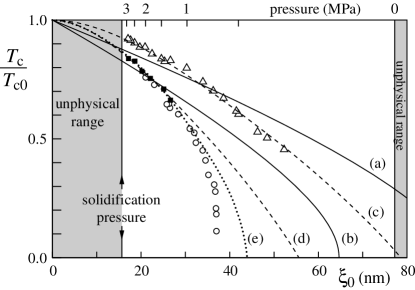
Figure 2: The transition temperature in aerogel relative to that in bulk, $T_{\rm c}/T_{\rm c0}$. The horizontal axis is the coherence length $\xi_{0}={\hbar v_{\rm f}/2\pi k_{\rm B}T_{\rm c0}}$. The experimentally inaccessible values of $\xi_{0}$ are denoted by shading. The data points are the same as in Fig. 1: Porto and Parpia (1995, △), Sprague et al. (1995,  ), and Matsumoto et al. (1997, $\circ$). The solid lines correspond to the homogeneous scattering model (HSM) at mean free paths $\ell_{\rm tr}=320$ nm (a) and 230 nm (b), and the dashed lines correspond to slabs of thicknesses $D=105$ nm (c) and 74 nm (d). The dotted line is the isotropic inhomogeneous scattering model (IISM) with average mean free path 70 nm, unit cell radius $R=140$ nm, and scattering profile parameter $j=8$.

The figure also shows the experimental data plotted as a function of the coherence length $\xi_{0}$. We see that the HSM gives a suppression of $T_{\rm c}$, but its dependence on $\xi_{0}$ is much weaker than is seen experimentally.

We have assumed in Fig. 2 that $\ell_{\rm tr}$ is a pressure-independent constant. We can identify three effects that could make $\ell_{\rm tr}=(n\sigma_{\rm tr})^{-1}$ pressure dependent. (i) The structure of aerogel changes. (ii) The Fermi momentum changes. (iii) The wave function of a quasiparticle changes. It seems that all these effects are negligible compared to the changes shown in Fig. 2. In particular, the Fermi momentum $\hbar k_{\rm f}$ changes only 10% over the whole pressure range, and calculations with hard spheres indicate that $\sigma_{\rm tr}$ is very weakly dependent on $k_{\rm f}$ for impurities that are large compared to $\lambda_{\rm f}$. What remains most uncertain is point (ii) because we do not know the wave function of a quasiparticle and how it changes with pressure.

In the neighborhood of the transition temperature $T_{\rm c}$ we expand $\alpha(T)=\alpha^{\prime}\times(T/T_{\rm c}-1)$. The higher order corrections in the Taylor series are dropped because they would not improve the accuracy of the GL functional (3). From equation (8) one easily gets

$$\alpha^{\prime}={N(0)\over 3}\left[1-x_{\rm c}\sum_{n=1}^{\infty}(n-{\textstyle{1\over 2}}+x_{\rm c})^{-2}\right]\ ,$$ (9)

where $x_{\rm c}=\hbar v_{\rm f}/4\pi T_{\rm c}\ell_{\rm tr}$.

It is not easy to calculate the fourth order coefficients $\beta_{i}$ with the same generality as $\alpha$. Therefore we make the additional assumption that only the $s$-wave scattering phase shift $\delta_{0}$ is nonzero. In this case $\sigma_{\rm tr}=\sigma$, and we get

$$\left(\matrix{\beta_{1}\cr\beta_{2}\cr\beta_{3}\cr\beta_{4}\cr\beta_{5}\cr}\right) = a\left(\matrix{-1/2\cr 1\cr 1\cr 1\cr-1\cr}\right)+b\left(\matrix{0\cr 1\cr 0\cr 1\cr-1\cr}\right)+\left(\matrix{\Delta\beta_{1}^{\rm sc}\cr\Delta\beta_{2}^{\rm sc}\cr\Delta\beta_{3}^{\rm sc}\cr\Delta\beta_{4}^{\rm sc}\cr\Delta\beta_{5}^{\rm sc}\cr}\right)$$ (10)

$$a = {N(0)\over 120(\pi T_{\rm c})^{2}}\sum_{n=1}^{\infty}(n-{\textstyle{1\over 2}}+x_{\rm c})^{-3}$$

$$b = {N(0)\hbar v_{\rm f}\over 288(\pi T_{\rm c})^{3}\ell}\left(\sin^{2}\delta_{0}-{\textstyle{1\over 2}}\right)\sum_{n=1}^{\infty}(n-{\textstyle{1\over 2}}+x_{\rm c})^{-4}\ .$$

Here $\Delta\beta_{j}^{\rm sc}$ are strong-coupling corrections which are not evaluated here. A model calculation for them in pure ³He is given by Sauls and Serene (1980).

Note that $\alpha$ and $a$, instead of depending separately on $n$ and the cross section $\sigma=(4\pi/k_{\rm f}^{2})\sin^{2}\delta_{0}$, depend only on the combination $\ell=(\sigma n)^{-1}$. This is not the case for $b$, which is also a function of $\delta_{0}$. The limiting cases $\sin^{2}\delta_{0}\rightarrow 0$ and $\sin^{2}\delta_{0}=1$ are known as Born and unitarity limits, respectively. This additional degree of freedom decreases the precision of the theoretical results because $\delta_{0}$ is not generally known. However, we argue in the following that this degree of freedom is averaged out in aerogel. Firstly, if the impurities are not identical, we can expect that there is a distribution of $\delta_{0}$’s instead of a single value. Secondly, the calculation including all partial waves has been done in the case of B phase ([TKR]). There one finds a similar spread of the results as a function of the phase shifts. But for large impurities the phase shifts $\delta_{l}$ with different $l$ are essentially random, as demonstrated by $\delta_{l}$ for hard spheres. Both these arguments support that a reasonable guess, if no more detailed information exists, is to assume random phase shifts $\sin^{2}\delta_{0}\rightarrow 0.5$.

A necessary condition for the stability of the A phase is $f_{\rm A}<f_{\rm B}$. Using equations (5), (7), and (10) this reduces to

$$a<6\Delta\beta_{1}^{\rm sc}+2\Delta\beta_{3}^{\rm sc}-4\Delta\beta_{45}^{\rm sc}\ .$$ (11)

Because $a$ increases monotonically by factor 3 with decreasing $T_{\rm c}$, the B phase becomes more favored with increasing scattering assuming that $\Delta\beta_{j}^{\rm sc}$ do not grow even more. Assuming $\Delta\beta_{j}^{\rm sc}$ remain constants, we can expect stable A phase only at temperatures (in mK) and pressures where it is stable in the pure case. Calculations with other phases indicate that they are not serious competitors to A and B phases.

In order to make more comparisons with experiments, we need to consider additional terms in the GL functional $F=\int d^{3}rf({\bf r})$. These are the gradient energy

$$f_{\rm k}=K\left[(\gamma-1)\partial_{i}A_{\mu i}\partial_{j}A_{\mu j}^{*}+\partial_{i}A_{\mu j}\partial_{i}A_{\mu j}^{*}\right]\ ,$$ (12)

the energy of the magnetic field ${\bf H}$,

$$f_{\rm z}=-{\textstyle{1\over 2}}\chi_{\rm n}^{-1}H^{2}+g_{\rm z}H_{\mu}A_{\mu i}A_{\nu i}^{*}H_{\nu}\ ,$$ (13)

where $\chi_{\rm n}$ is the susceptibility of the normal state, and the magnetic dipole-dipole interaction energy

$$f_{\rm d}=g_{\rm d}(|A_{ii}|^{2}+A_{ij}A_{ji}^{*}-{\textstyle{2\over 3}}A_{\mu i}A_{\mu i}^{*})\ .$$ (14)

Here $f_{\rm k}$ is purely phenomenological similar to the bulk energy (3), but in $f_{\rm z}$ and $f_{\rm d}$ we have dropped some terms, which could be there in a pure phenomenological theory. For the coefficients we calculate (Appendix)

$$K = {N(0)\hbar^{2}v_{\rm f}^{2}\over 240\pi^{2}T_{\rm c}^{2}}\sum_{n=1}^{\infty}(n-{\textstyle{1\over 2}}+x_{\rm c})^{-3}$$ (15)

$$\gamma = 3+{5\hbar v_{\rm f}\over 12\pi T_{\rm c}\ell}{\sum_{n=1}^{\infty}(n-{1\over 2})^{-1}(n-{1\over 2}+x_{\rm c})^{-3}\over\sum_{n=1}^{\infty}(n-{1\over 2}+x_{\rm c})^{-3}}$$ (16)

$$g_{\rm z} = {\hbar^{2}\tilde{\gamma}^{2}N(0)\over 48\pi^{2}T_{\rm c}^{2}(1+F_{0}^{\rm a})^{2}}\sum_{n=1}^{\infty}(n-{\textstyle{1\over 2}}+x_{\rm c})^{-3}$$ (17)

$$g_{\rm d} = {\mu_{0}\over 40}\left[\hbar\tilde{\gamma}N(0)R\sum_{n=1}^{\epsilon_{\rm cut\,off}/2\pi T_{\rm c}}(n-{\textstyle{1\over 2}}+x_{\rm c})^{-1}\right]^{2},$$ (18)

where $\tilde{\gamma}$ is the gyromagnetic ratio, $F_{0}^{\rm a}$ a Fermi-liquid parameter, $R$ a renormalization constant for the dipole energy, and $\epsilon_{\rm cut\,off}$ a high-energy cut-off ([Leggett]). The dipole-dipole coupling constant $g_{\rm d}$ is different form the other coefficients [(8)-(10), (15)-(17)] because it is dominated by high-energy processes (it would diverge for $\epsilon_{\rm cut\,off}\rightarrow\infty$), and therefore it is a constant (independent of scattering).

All the coefficients above reduce to the well know GL coefficients in the limit vanishing scattering, $\ell\rightarrow\infty$ (Fetter 1975, [T87]).

In most cases the terms $f_{\rm z}$ and $f_{\rm d}$ are small compared to $f_{\rm bulk}$. Treating them as perturbations, we find in the A phase (apart from constants)

$$f_{\rm zA} = -{\textstyle{1\over 2}}\chi_{\rm n}^{-1}H^{2}+g_{\rm z}\Delta_{\rm A}^{2}(\hat{\bf d}\cdot{\bf H})^{2}$$ (19)

$$f_{\rm dA} = -2g_{\rm d}\Delta_{\rm A}^{2}(\hat{\bf d}\cdot\hat{\bf l})^{2}\ ,$$ (20)

which favor $\hat{\bf d}\perp{\bf H}$ and $\hat{\bf d}\parallel\hat{\bf l}$, respectively. The B phase is slightly more complicated. We parameterize the rotation matrix $R_{\mu i}$ by an angle $\theta$ and an axis $\hat{\bf n}$ of rotation. The dipole-dipole energy $f_{\rm d}$ favors $\theta={\rm arccos}(-1/4)=104^{\circ}$. The external field leads to distortion of B phase order parameter (4). This gives rise to the energy term

$$f_{\rm dzB}=-{5g_{\rm d}g_{\rm d}\over 4\beta_{345}}(\hat{\bf n}\cdot{\bf H})^{2}\ ,$$ (21)

which favors $\hat{\bf n}\parallel{\bf H}$.

For comparison to experiments, we still need to relate the observables to the GL coefficients. The torsional oscillator experiments measure the superfluid density $\rho_{\rm s}$ ([Porto, Matsumoto]). This can be calculated by evaluating $f_{\rm k}$ (12) in the presence of a phase gradient: ${\mbox{\boldmath$\nabla$}}A_{\mu j}=i{\bf q}A_{\mu j}$, where the superfluid velocity ${\bf v}_{\rm s}=\hbar{\bf q}/2m_{3}$ and $m_{3}$ is the mass of a ³He atom. The main quantities measured in the NMR experiment are the magnetic susceptibility $\chi$ and the shift of the resonance frequency $\delta\omega$ from the Larmor value. The former is obtained by evaluating $f_{\rm z}$. The latter needs evaluating $f_{\rm d}$ in the dynamic case ([Leggett]). The results for homogeneous A and B phases are

$$\rho_{\rm sA} = {8m_{3}^{2}\over\hbar^{2}}K\Delta_{\rm A}^{2}[\gamma+1-(\gamma-1)(\hat{\bf l}\cdot\hat{\bf v}_{\rm s})^{2}]$$ (22)

$$\rho_{\rm sB} = {8m_{3}^{2}\over\hbar^{2}}(\gamma+2)K\Delta_{\rm B}^{2}$$ (23)

$$\chi_{\rm A} = \chi_{\rm n}\ \ \ \ \ \ \ \ \ \ \ \ \ \ \ \ \ \ \ \ \ \ \ \ \ \ \ \ \ \ \ \ \ \ \ \ \ \ \ \ \ \ \ \ \ \ \ \ \ \ (\hat{\bf d}\perp{\bf H})$$ (24)

$$\chi_{\rm B} = \chi_{\rm n}-2g_{\rm z}\Delta_{\rm B}^{2}$$ (25)

$$\delta\omega_{\rm A} = {2\tilde{\gamma}\over\chi_{\rm n}H}g_{\rm d}\Delta_{\rm A}^{2}[(\hat{\bf l}\cdot\hat{\bf d})^{2}-(\hat{\bf l}\cdot\hat{\bf H})^{2}]\ \ \ \ \ \ \ \ \ \ \ \ \ \ \ \ (\hat{\bf d}\perp{\bf H})$$ (26)

$$\delta\omega_{\rm B} = {15\tilde{\gamma}\over 2\chi_{\rm n}H}g_{\rm d}\Delta_{\rm B}^{2}|\hat{\bf n}\times\hat{\bf H}|^{2}\ \ \ \ \ \ \ \ \ \ \ \ \ \ \ \ \ \ \ \ \ \ \ \ \ (\theta=104^{\circ})\ .$$ (27)

Here $\hat{\bf v}_{\rm s}$ and $\hat{\bf H}$ denote the directions of the superfluid velocity and field, respectively. The susceptibility of the normal phase $\chi_{\rm n}$ has to include the inert layer of ³He atoms on the aerogel strands, which in fact is the dominant contribution at low temperatures ([Sprague1]). The frequency shifts $\delta\omega$ are for small tipping angles of the magnetization from the equilibrium direction $\hat{\bf H}$, and the magnetic field $H$ is assumed large in comparison to $\sqrt{g_{\rm d}/g_{\rm z}}\approx 0.2$ mT. The results for $\chi_{\rm A}$, $\delta\omega_{\rm A}$, and $\delta\omega_{\rm B}$ are limited to the conditions indicated in parenthesis after each equation.

The NMR experiments with ³He (no ⁴He mixed) see no deviation of the susceptibility from $\chi_{\rm n}$ ([Sprague1], 1996). In the HSM model, we interpret this as evidence for the A phase. Therefore, the measured frequency shift is best compared with $\delta\omega_{\rm A}$. In Fig. 3(a) we plot the suppression factor

$$S_{\chi_{\rm n}\delta\omega_{\rm A}}\equiv{\chi_{\rm n}\delta\omega(tT_{\rm c})\over\chi_{\rm n0}\delta\omega_{\rm A0}(tT_{\rm c0})}={\Delta^{2}(tT_{\rm c})\over\Delta_{0}^{2}(tT_{\rm c0})}\equiv S_{\Delta^{2}}\ .$$ (28)

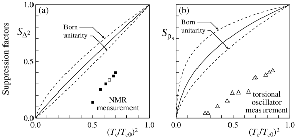
Figure 3: The suppression factors for $\Delta^{2}$ and $\rho_{s}$ as a function of $T_{\rm c}$ reduction: $(T_{\rm c}/T_{\rm c0})^{2}$. The lines are theoretical results for the B phase when $t\rightarrow 1$ [see equations (28) and (29)]. The dashed lines denote Born and unitarity limits, and solid lines are for the intermediate case $\sin^{2}\delta_{0}=0.5$. The data points are from Sprague et al. (1995, A type phase,  ), Sprague et al. (1996, B type phase,    ), and Porto and Parpia (1995, △), all corresponding to $t\approx 0.9$.

Generally, the suppression factor is the ratio of a quantity in aerogel relative to the same quantity in the pure case. The latter is denoted by subindex $0$. The ratio is taken at the same temperature $t$ measured relative to the corresponding $T_{\rm c}$. We consider here $t$ in the range $0.9\ldots 1$ where the GL theory is expected to be valid. The middle equality (28) is based on equation (26). It is valid because $g_{\rm d}$ is a constant and the minimum-energy orientations of $\hat{\bf d}$ and $\hat{\bf l}$ are unchanged by scattering. (The latter is not necessarily satisfied in generalizations of the HSM, see Section 6.) Similarly we can define a suppression factor for $\rho_{\rm s}$:

$$S_{\rho_{\rm s}}\equiv{\rho_{\rm s}(tT_{\rm c})\over\rho_{\rm s0}(tT_{\rm c0})}\ .$$ (29)

The B phase $\rho_{\rm s0}$ is used as a reference in the experimental points of Fig. 3(b).

The theoretical suppression factors $S_{\Delta^{2}}$ and $S_{\rho_{\rm s}}$ are plotted in Fig. 3. In these the impure B phase is compared with bulk B phase. Very similar suppression factors are obtained when impure A phase is compared with bulk A phase: The solid lines are the same for $\Delta^{2}$ and also for $\rho_{\rm s}$ (22) averaged over all orientations of the A phase [corresponding to $(\hat{\bf l}\cdot\hat{\bf v}_{\rm s})^{2}\rightarrow{1\over 3}$]. The variation between Born and unitarity limits is slightly smaller in the A than in the B phase.

We see from Fig. 3 that HSM indeed gives a suppression of $\Delta^{2}$ and $\rho_{\rm s}$, but it is insufficient to explain quantitatively the measured suppression.

5 Inhomogeneous scattering models

The disagreement between the experiments and the HSM is clear in Fig. 3. We have checked that this failure does not arise from limitation to the neighborhood of $T_{\rm c}$ or to the $s$-wave scattering approximation. Also magnetic scattering does not seem to give a solution to this problem. We also discuss in Section 6 that the problem cannot be explained away by random anisotropy of the aerogel. Therefore it seems inevitable to sacrifice to basic assumption of the HSM: the homogeneity of the scattering.

A simple model of inhomogeneous scattering is to consider ³He between two diffusively scattering planes. The transition temperature for this “slab model” is calculated by Kjäldman et al. (1978), and the suppression factors are evaluated by Thuneberg et al. (1996). This gave promising results (see Fig. 2) but it is not a suitable model for aerogel because of its strong anisotropy. Recently an “isotropic inhomogeneous scattering model” (IISM) was studied ([letter]). This is consistent with the observed isotropy of aerogel, and it gives rather good fits to both $T_{\rm c}$ and $S_{\Delta^{2}}$. Because only preliminary calculations on the IISM has been done, we leave its discussion to another occasion. What is of importance here that part of the HSM seems to remain valid: Although the gap amplitude $\Delta^{2}$ is badly overestimated in the HSM, the equations (22)-(27) for $\rho_{s}$, $\chi$, and $\delta\omega$ may still constitute a reasonable approximation. This will be used in the following section. Similar arguments may be applied to the HSM calculations by Baramidze et al. (1996).

6 Anisotropic HSM

In this section we consider how to generalize the isotropic HSM (Section 4) to anisotropic scattering. The anisotropy will affect all the terms in the GL functional, but the most important effect comes from the modification of the second order bulk term (3). The anisotropy requires the replacement

$$\alpha A_{\mu i}^{*}A_{\mu i}\rightarrow\alpha_{ij}A_{\mu i}^{*}A_{\mu j}\ .$$ (30)

So the scalar $\alpha$ is replaced by a tensor ${\underline{\alpha}}$. Solving the quasiclassical equations in this case gives

$${\underline{\alpha}}={N(0)\over 3}\left\{\ln{T\over T_{\rm c0}}+\sum_{m=1}^{\infty}\left[{1\over m-{1\over 2}}-\left(m-{\textstyle{1\over 2}}+{\hbar v_{\rm f}n\over 4\pi T}{\underline{\sigma}}_{\rm tr}\right)^{-1}\right]\right\}\ .$$ (31)

Unit matrices multiplying $m-{1\over 2}$, for example, are not shown explicitly. The transport cross-section tensor is defined by the double angular average

$${\underline{\sigma}}_{\rm tr}=\langle\,\hat{\bf k}\left[\sigma(\hat{\bf k})\hat{\bf k}-4\pi\langle{d\sigma\over d\Omega}(\hat{\bf k},\hat{\bf k}^{\prime})\hat{\bf k}^{\prime}\rangle_{\hat{\bf k}^{\prime}}\right]\rangle_{\hat{\bf k}}\ ,$$ (32)

where $d\sigma/d\Omega$ is the differential scattering cross section and the total cross section $\sigma(\hat{\bf k})=4\pi\langle(d\sigma/d\Omega)(\hat{\bf k},\hat{\bf k}^{\prime})\rangle_{\hat{\bf k}^{\prime}}$. [In equation (31) we have assumed that both $\hat{\bf k}$ and $\hat{\bf k}^{\prime}$ dependencies of $(d\sigma/d\Omega)(\hat{\bf k},\hat{\bf k}^{\prime})$ can be represented by $s$ and $p$-wave spherical harmonic functions.] For estimation of the anisotropy in aerogel we consider a long rod, which scatters diffusely (randomly) the particles hitting it. This gives $n{\underline{\sigma}}_{\rm tr}=\ell^{-1}({9\over 8}-{3\over 8}\hat{\bf a}\hat{\bf a})$, where $\hat{\bf a}$ is the direction of the rod and $\ell$ denotes the average (transport) mean free path. Assuming the anisotropy is small, the leading effect of the anisotropy can be represented by

$$f_{\rm a}=-\alpha_{1}\hat{a}_{i}A_{\mu i}^{*}A_{\mu j}\hat{a}_{j}\ ,$$ (33)

where

$$\alpha_{1}={N(0)\hbar v_{\rm f}\over 32\pi T_{\rm c}\ell}\sum_{m=1}^{\infty}(m-{\textstyle{1\over 2}}+x_{\rm c})^{-2}.$$ (34)

It is crucial that the anisotropy direction $\hat{\bf a}$ is not a constant. We expect that the orientational correlation decays in a length $L_{\rm a}\sim 20$ nm, which is on the order of the average distance between strands.

The anisotropy (33) shifts the transition temperature. It also changes the relative stability of different phases. Instead of discussing these, we will here concentrate on how the anisotropy can crucially modify the NMR properties. Some of the ideas below are suggested by Volovik (1996).

Quite generally, we can write the following hydrodynamic free energy for the A phase

$$f_{\rm A} = -{\textstyle{1\over 2}}\lambda_{\rm d}(\hat{\bf d}\cdot\hat{\bf l})^{2}+{\textstyle{1\over 2}}\lambda_{\rm z}(\hat{\bf d}\cdot{\bf H})^{2}+{\textstyle{1\over 2}}\lambda_{\rm a}(\hat{\bf a}\cdot\hat{\bf l})^{2}+{\textstyle{1\over 2}}\rho_{\perp}{\bf v}_{\rm s}^{2}+{\textstyle{1\over 2}}(\rho_{\parallel}-\rho_{\perp})(\hat{\bf l}\cdot{\bf v}_{\rm s})^{2}$$ (35)

$$+C{\bf v}_{\rm s}\cdot\nabla\times\hat{\bf l}-C_{0}(\hat{\bf l}\cdot{\bf v}_{\rm s})(\hat{\bf l}\cdot\nabla\times\hat{\bf l})+{\textstyle{1\over 2}}K_{\rm s}(\nabla\cdot\hat{\bf l})^{2}+{\textstyle{1\over 2}}K_{\rm t}(\hat{\bf l}\cdot\nabla\times\hat{\bf l})^{2}$$

$$+{\textstyle{1\over 2}}K_{\rm b}|\hat{\bf l}\times(\nabla\times\hat{\bf l})|^{2}+{\textstyle{1\over 2}}K_{5}|(\hat{\bf l}\cdot\nabla)\hat{\bf d}|^{2}+{\textstyle{1\over 2}}K_{6}[(\hat{\bf l}\times\nabla)_{i}\hat{\bf d}_{j})]^{2}\ .$$

The first two terms are already familiar from equations (19) and (20). The third is the anisotropy term (33) with $\lambda_{\rm a}=2\alpha_{1}\Delta_{\rm A}^{2}$. The rest arises from the gradient energy (12) when the A-phase order parameter (6) is substituted into it ([Cross]). All the coefficients are proportional to $\Delta_{\rm A}^{2}$. Because this common factor drops out in relative comparisons of the terms, our estimations below are independent of $\Delta_{\rm A}^{2}$.

The idea is that the random field $\hat{\bf a}$ tries to orient the $\hat{\bf l}$ vector. However, the gradient energy strongly limits the variation of $\hat{\bf l}$ on the scale $L_{\rm a}$. Instead, $\hat{\bf l}$ varies only on a “orbital” scale $L_{\rm o}\gg L_{\rm a}$. In addition, the $\hat{\bf d}$ vector varies on a “spin” scale $L_{\rm s}$, which also is large in comparison to “aerogel” scale $L_{\rm a}$. We estimate $L_{\rm o}$ and $L_{\rm s}$ using arguments presented by Imry and Ma (1975). The exact functional (35) is approximated by

$$f_{\rm A} \approx -{\lambda_{\rm d}\over 6}-{\eta\lambda_{\rm d}\over 3\eta+2[({L_{\rm s}/L_{\rm o}})^{3/4}-1]^{2}}$$ (36)

$$\hbox{}+{\lambda_{\rm a}\over 6}-{\eta\lambda_{\rm a}\over 2}\left({L_{\rm a}\over L_{\rm o}}\right)^{3/2}+{K_{\rm s}\over 2L_{\rm s}^{2}}+{K_{\rm o}\over 2L_{\rm o}^{2}}\ .$$

This is a functional of only two variables, $L_{\rm s}$ and $L_{\rm o}$. The first two terms constitute an interpolation of the dipole-dipole energy between two limits. The minimum energy $-{1\over 2}\lambda_{\rm d}$ is obtained in the limit $L_{\rm s}=L_{\rm o}$. In the opposite limit $L_{\rm s}\gg L_{\rm o}$, the dipole-dipole energy consists of a random average $-{1\over 6}\lambda_{\rm d}$ plus a fluctuation $-{1\over 2}\eta\lambda_{\rm d}(L_{\rm o}/L_{\rm s})^{3/2}$ ([IM]). The origin of the factor $(L_{\rm o}/L_{\rm s})^{3/2}$ is that in a box of volume $L_{\rm s}^{3}$ there are $N=(L_{\rm o}/L_{\rm s})^{3}$ uncorrelated regions of $\hat{\bf l}$, and therefore the total fluctuation they produce is proportional $\sqrt{N}$. Here $\eta=2/3\sqrt{5}$ is the standard deviation of $(\hat{\bf n}\cdot\hat{\bf z})^{2}$ for a random unit vector $\hat{\bf n}$. The third and fourth terms in (36) approximate similarly the anisotropy energy ${1\over 2}\lambda_{\rm a}(\hat{\bf a}\cdot\hat{\bf l})^{2}$, but there only the limiting form $L_{\rm o}\gg L_{\rm a}$ is needed. The last two terms are simplified gradient energies of $\hat{\bf d}$ and $\hat{\bf l}$. We assume $K_{\rm s}\approx 12K\Delta_{\rm A}^{2}$ and $K_{\rm o}\approx 6K\Delta_{\rm A}^{2}$, where a factor 3 arises from the dimensionality of the space.

The simplified energy functional can now be trivially minimized numerically, and also to a great extent analytically. We find two basically different solutions, which are described below. These solutions have equal energy if $L_{\rm a}=48$ nm, which is only slightly larger than the estimated distance between stands 20 nm. The numerical estimates use this and the pressure of 2.8 MPa.

In the “dipole locked” solution $\hat{\bf d}$ and $\hat{\bf l}$ follow closely each other, $\hat{\bf d}({\bf r})\approx\hat{\bf l}({\bf r})$. We find rather long $L_{\rm s}\approx L_{\rm o}\approx 70\ \mu$m. The NMR experiments are done in large magnetic field, so that $\hat{\bf d}\approx\hat{\bf l}$ is allowed to vary only in the plane perpendicular to ${\bf H}$. We see from equation (26) that the NMR frequency shift $\delta\omega_{\rm A}$ is essentially unchanged from the HSM prediction. This state has lowest energy for $L_{\rm a}<48$ nm.

In the “dipole unlocked” solution $\hat{\bf l}$ varies on a much shorter scale than $\hat{\bf d}$, $L_{\rm o}\ll L_{\rm s}$. We find $L_{\rm o}\approx 8\ \mu$m and $L_{\rm s}\approx 3$ mm. Again the magnetic field limits $\hat{\bf d}$ to the plane perpendicular to ${\bf H}$. However, $\hat{\bf l}$ is free to vary in all directions. The NMR frequency shift is totally suppressed: it is reduced by factor $10^{-5}$ relative to the HSM. This is because $\langle(\hat{\bf l}\cdot\hat{\bf d})^{2}\rangle\approx\langle(\hat{\bf l}\cdot\hat{\bf H})^{2}\rangle\approx{1\over 3}$ in the expression for $\delta\omega_{\rm A}$ (26). This state has lowest energy if $L_{\rm a}>48$ nm.

As discussed above, the experiments see that the NMR frequency shift is smaller than the HSM prediction. However, they still are on the same order of magnitude. This strongly supports the dipole-locked state because in the unlocked state the suppression would be much more severe. Moreover, because the suppression in the locked state is unchanged from HSM, we reach the conclusion (stated in Section 5) that random anisotropy cannot explain the difference between measurements and the HSM.

The presence of the dipole-locked state of ³He in aerogel implies that the anisotropy of aerogel is very small: it is equivalent to rods whose directions are correlated over distance $L_{\rm a}<48$ nm. This invalidates the slab model, because the thickness $D$ of the slab is larger that this (see Fig. 2).

Above we have considered the NMR properties only in the case that the “tipping angle” $\beta$ between the field and the magnetization is small. When the angle is increased, the frequency shift $\delta\omega$ gradually diminishes. This is similar to bulk ³He-A, and it is well understood theoretically ([BS, Fomin]). However, the frequency shift suddenly disappears at about $\beta=40^{\circ}$, and remains zero for all larger angles ([Sprague1]). As suggested by Volovik (1996), this striking observation can be associated with the locked$\rightarrow$unlocked transition discussed above. At the time of writing this, this is still under study, so we postpone the discussion to another occasion.

7 Conclusion

We have extensively studied the homogeneous scattering model in the Ginzburg-Landau approximation. Although it fails to produce the correct gap amplitude, it may successfully applied in the hydrodynamic region. As an example we considered NMR in the A phase. In the future it could be used, e.g., for studying vortices of ³He in aerogel.

Appendix

In this appendix we briefly explain how the Ginzburg-Landau coefficients ($\alpha$, $\beta_{i}$, etc.) are calculated in the quasiclassical theory. An intermediate quantity in the calculation is the quasiclassical $4\times 4$ matrix Green’s function $\hat{g}(\hat{\bf k},{\bf r},\epsilon_{m})$. The arguments are the direction of the momentum $\hat{\bf k}$, the location ${\bf r}$, and the Matsubara frequencies $\epsilon_{m}=\pi k_{\rm B}T(2m+1)$. The Green’s function is determined from the Eilenberger equations

$$[i\epsilon_{m}\hat{\tau}_{3}-\hat{\nu}-\hat{\rho}-\hat{\Delta},\hat{g}]+iv_{\rm F}\hat{\bf k}\cdot\mbox{\boldmath$\nabla$}_{\bf r}\hat{g}=0$$ (37)

$$\hat{g}\hat{g}=-\pi^{2}\ .$$ (38)

Here $\hat{\tau}_{i}$ denote the Pauli matrices in Nambu space, and $[A,B]=AB-BA$. For more details the reader is referred to the review article by Serene and Rainer (1983). The self-consistency equations for the diagonal $\hat{\nu}$ and off-diagonal $\hat{\Delta}$ self energies are given in formulas (5.10) of Serene and Rainer (1983). The impurity self-energy $\hat{\rho}(\hat{\bf k},{\bf r},\epsilon_{m})$ equals $n({\bf r})\hat{t}(\hat{\bf k},\hat{\bf k},{\bf r},\epsilon_{m})$, where $n({\bf r})$ is the concentration of the scattering centers. The $\hat{t}$-matrix of a single scattering center is determined by

$$\hat{t}(\hat{\bf k},\hat{\bf k}^{\prime},{\bf r},\epsilon_{m}) = \hat{v}(\hat{\bf k},\hat{\bf k}^{\prime})+N(0)\langle\hat{v}(\hat{\bf k},\hat{\bf k}^{\prime\prime})\hat{g}(\hat{\bf k}^{\prime\prime},{\bf r},\epsilon_{m})\hat{t}(\hat{\bf k}^{\prime\prime},\hat{\bf k}^{\prime},{\bf r},\epsilon_{m})\rangle_{\hat{\bf k}^{\prime\prime}}\ .$$ (39)

Also we need the free energy functional which is given by equation (5.11) of Serene and Rainer (1983).

The coefficients are calculated by solving Green’s function perturbatively $\hat{g}=\hat{g}_{0}+\hat{g}_{1}+\hat{g}_{2}+\ldots$. Here $\hat{g}_{0}$ is the normal state Green’s function, and the subindex denotes order in $\hat{\Delta}$. Then one collects terms of order 0, 1, 2, and 3 in the Eileberger, self-consistency and $\hat{t}$-matrix equations, and solves them in each order. Substitution to energy functional gives the results $\alpha$ (8) and $\beta_{i}$ (10). For other coefficients it is sufficient to limit to first order in $\hat{\Delta}$, but one has to do additional expansions in gradients and in magnetic field. Substitution to energy functional gives $K$ (15), $\gamma$ (16) and $g_{\rm z}$ (17). The dipole coefficient (18) is obtained using the dipole-dipole Hamiltonian ([Leggett]) in the general energy functional (5.6) of Serene and Rainer (1983).

References

- [1] AGAbrikosov and Gorkov 1961 Abrikosov A.A., Gorkov L.P. (1961): Zh. Eksp. Teor. Fiz. 39, 1781 [Sov. Phys. JETP 12, 1243 (1961)]
- [2] BKVBaramidze et al. 1996 Baramidze G., Kharadze G., Vachnadze G. (1996): Pisma Zh. Eksp. Teor. Fiz. 63, 95 [JETP Lett. 63, 107]
- [3] BSBrinkman and Smith 1975 Brinkman W.F., Smith H. (1975): Phys. Lett. A 51, 449
- [4] BRBuchholtz and Rainer 1979 Buchholtz L.J., Rainer D. (1979): Z. Physik B 35, 151
- [5] CrossCross 1975 Cross M.C. (1975): J. Low Temp. Phys. 21, 525
- [6] F75 Fetter A.L. (1975):Quantum Statistics and the Many-Body Problem, eds. S.B. Trickey, W.P. Kirk and J.W. Dufty (Plenum, New York), 127
- [7] FominFomin 1978 Fomin I.A. (1978): J. Low Temp. Phys. 31, 509
- [8] FrickeSciAmFricke 1988 Fricke J. (1988): Sci. Am. 258, No. 5, 68
- [9] GorkovGorkov 1959 Gorkov L.P. (1959): Zh. Eksp. Teor. Fiz. 37, 1407 [Sov. Phys. JETP 37, 998 (1960)]
- [10] IMImry and Ma 1975 Imry Y., Ma S. (1975): Phys. Rev. Lett. 35, 1399
- [11] KMCKim et al. 1993 Kim S.B., Ma J., Chan M.H.W. (1993): Phys. Rev. Lett. 71, 2268
- [12] KKRKjäldman et al. 1978 Kjäldman L.H., Kurkijärvi J., Rainer D. (1978): J. Low Temp. Phys. 33, 577
- [13] larkinLarkin 1965 Larkin A.I. (1965): JETP Lett. 2, 130
- [14] LeggettLeggett 1974 Leggett A.J. (1974): Ann. Phys. 85, 11
- [15] LeggettRMPLeggett 1975 Leggett A.J. (1975): Rev. Mod. Phys. 47, 331
- [16] MatsumotoMatsumoto et al. 1997 Matsumoto K., Porto J.V., Pollack L., Smith E.N., Ho T.L., Parpia J.M. (1997): Phys. Rev. Lett. 79, 253
- [17] MerminSMermin and Stare 1973 Mermin N.D., Stare C. (1973): Phys. Rev. Lett. 30, 1135
- [18] PortoPorto and Parpia 1995 Porto J.V., Parpia J.M. (1995): Phys. Rev. Lett. 74, 4667
- [19] SSSauls and Serene 1981 Sauls J.A., Serene J.W. (1981): Phys. Rev. B 24, 183
- [20] SRrevSerene and Rainer 1983 Serene J.W., Rainer D. (1983): Phys. Rep. 101, 221
- [21] Sprague1Sprague et al. 1995 Sprague D.T., Haard T.M., Kycia J.B., Rand M.R., Lee Y., Hamot P.J., Halperin W.P. (1995): Phys. Rev. Lett. 75, 661
- [22] Sprague2Sprague et al. 1996 Sprague D.T., Haard T.M., Kycia J.B., Rand M.R., Lee Y., Hamot P.J., Halperin W.P. (1996): Phys. Rev. Lett. 77, 4568
- [23] TholenParpiaTholen and Parpia 1992 Tholen S.M., Parpia J.M. (1992): Phys. Rev. Lett. 68, 2810
- [24] T87Thuneberg 1987 Thuneberg E.V. (1987): Phys. Rev. B 36, 3583
- [25] TKRThuneberg et al. 1981 Thuneberg E.V., Kurkijärvi J., Rainer D. (1981): J. Phys. C 14, 5615
- [26] LTPragThuneberg et al. 1996 Thuneberg E.V., Fogelström M., Yip S.K., Sauls J.A. (1996): Czechoslovak J. Phys. 46, 113
- [27] letterThuneberg et al. 1997 Thuneberg E.V., Fogelström M., Yip S.K., Sauls J.A. (1997): http://xxx.lanl.gov /abs/cond-mat/9601148
- [28] 3HereviewVollhardt and Wölfle 1990 Vollhardt D., Wölfle P. (1990): The superfluid phases of helium 3 (Francis&Taylor, London)
- [29] VolovikVolovik 1996 Volovik G.E. (1996): Pis’ma Zh. Eksp. Teor. Fiz. 63, 281