[

Effects of Noise in Symmetric Two-Species Competition

Abstract

We have analyzed the interplay between noise and periodic modulations in a classical Lotka-Volterra model of two-species competition. We have found that the consideration of noise changes drastically the behavior of the system and leads to new situations which have no counterpart in the deterministic case. Among others, noise is responsible for temporal oscillations, spatial patterns, and the enhancement of the response of the system via stochastic resonance.

]

In the last years the study of deterministic mathematical models of ecosystems has clearly revealed a large variety of phenomena, ranging from deterministic chaos to the presence of a spatial organization [1, 2, 3, 4]. In the absence of spatial dependence these models study the time evolution of the averaged number of individuals of some interacting species. When space is considered, the description is usually done in terms of population density fields. These models, however, do not account for the effects of noise despite it is always present in actual population dynamics and arises from different sources, such as the intrinsic stochasticity associated to the dynamics of the individuals and the random variability of the environment [5]. Frequently, its effects have been assumed to be only a source of disorder[6]. Conversely, in this Letter we show how the consideration of noise in a classical Lotka-Volterra model of two species competition changes drastically and in an unexpected fashion the dynamics of the deterministic case. Moreover, consideration of noise and space together leads to the appearance of spatiotemporal patterns which in the deterministic model, except for an initial transient and no matter the value of the parameters, always looks homogeneous.

Let us consider a classical Lotka-Volterra model of symmetric two-species competition[7, 2] with the addition of noise terms[5] defined by the equations

$${dx\over dt} = \mu x(1-x-\beta y)+f_{x}(x,y)\xi_{x}(t)\;\;,$$ (1)

$${dy\over dt} = \mu y(1-y-\beta x)+f_{y}(x,y)\xi_{y}(t)\;\;,$$ (2)

where $x$ and $y$ are the population densities, $\mu$ is proportional to the growth rate, and $\beta$ accounts for the interactions among the species. Here the terms $f_{i}(x,y)\xi_{i}(t)$ ($i=x,y$) model the contribution of the random forces. For the sake of simplicity we assume that $f_{x}(x,y)=x$, $f_{y}(x,y)=y$. Moreover, $\xi_{i}(t)$ is assumed Gaussian white noise with zero mean and correlation function $\left<\xi_{i}(t)\xi_{j}(t+\tau)\right>=\sigma\delta(\tau)\delta_{i,j}$ ($i,j=x,y$). This explicit form of the noise term may represent, for instance, a fluctuating growth rate. Without the noise terms this Lotka-Volterra model has been widely studied and it is well know that, for $\beta<1$, both species are present but for $\beta>1$, exclusion takes place through a symmetry-breaking bifurcation and one of the species is eliminated.

FIG. 1.: (a) Time evolution of both population densities [Eqs. (1) and (2)]. The values of the parameters are $\mu=1$, $\omega_{0}/2\pi=10^{-3}$, $\alpha=0.05$, $\varepsilon=-0.01$, and $\sigma=10^{-12}$. (b) Same situation as in case (a) but $\sigma=10^{-6}$. (c) and (d) Same situation as in case (a) but $\sigma=10^{-2}$.

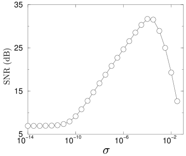
FIG. 2.: SNR corresponding to Eqs. (1) and (2). The values of the parameters are $\mu=1$, $\omega_{0}/2\pi=10^{-3}$, $\alpha=0.05$, and $\varepsilon=-0.01$

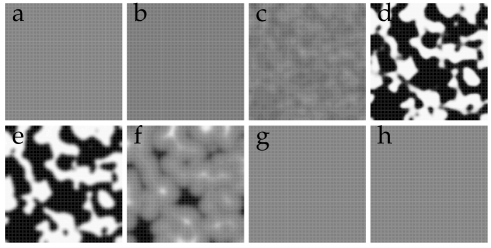
FIG. 3.: Representation of $x^{n}_{i,j}$ given through Eqs. (5) and (7) for $n=1750$ (a), $n=1875$ (b), $n=2000$ (c), $n=2125$ (d), $n=2250$ (e), $n=2375$ (f), $n=2500$ (g), and $n=2625$ (h). The values of the parameters are $\mu=2$, $D=0.05$, $\omega_{0}/2\pi=10^{-3}$, $\alpha=0.1$, $\varepsilon=-0.01$, and $\sigma=10^{-8}$. The system size is $200\times 200$. Black and white colors stand for minimum and maximum values, respectively.

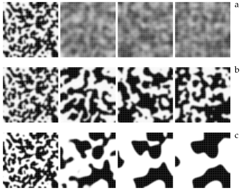
FIG. 4.: (a) Representation of $x^{n}_{i,j}$ given through Eqs. (5) and (7) for $n=250,1250,2250,3250$ (from left to right). The values of the parameters are $\mu=2$, $D=0.05$, $\omega_{0}/2\pi=10^{-3}$, $\alpha=0.1$, $\varepsilon=-0.01$, and $\sigma=10^{-12}$. The system size is $200\times 200$. Black and white colors stand for minimum and maximum values, respectively. (b) Same situation as in case (a) but $\sigma=10^{-8}$. (c) Same situation as in case (a) but $\sigma=0$ and $\varepsilon=0.01$.

As an additional feature, we account for a non-stationary environment. The simplest way to do it is to assume that our dynamics is modulated through a periodic variation in one of the relevant parameters. Seasonality and daily variations are the most important sources of regular forcing. The explicit case we consider here is described by

$$\beta\equiv\beta(t)=1+\varepsilon+\alpha\sin(\omega_{0}t)\;\;,$$ (3)

where $\varepsilon$, $\alpha$ and $\omega_{0}$ are constants. This form of $\beta(t)$ corresponds to a situation in which the competition between species is altered in such a way that we move from coexistence ($\beta<1$) to exclusion ($\beta>1$) in a regular fashion. The change in the competition rate may occur when a limiting resource which is used by both populations goes from large to low values. Thus, at high levels, competition is weak, but can become strong at low levels.

Although some Lotka-Volterra models with sinusoidal perturbations of parameters show very complex dynamical patterns[8], in the model we consider the situation is rather simple. In the absence of noise, except for a possible initial transient, when $\varepsilon>0$ exclusion takes place. On the other hand, when $\varepsilon<0$ the species always coexist, in spite of the fact that $\beta$ becomes larger than $1$ periodically in time. The introduction of noise drastically changes the previous scenario since even small amounts of stochasticity are able to destroy the state of coexistence periodically[9]. In order to analyze our system we have numerically integrated the previous equations by using standard methods for stochastic differential equations [10]. In Fig. 1a we have plotted the temporal evolution of both species when $\varepsilon<0$ and the noise level $\sigma$ is very small, but its effects are slightly appreciable. Thus, the species practically coexist all the time. When noise increases sufficiently a species is able to nearly exclude the other one periodically (see Fig. 1b), i.e., one species dominates the other. It is interesting to realize that by increasing even more the noise level this coherent response to environmental variations is lost (See Figs. 1c and 1d). A nontrivial consequence of these results is that time variations in competing populations could be a noise-induced phenomenon. In this context, periodic population oscillations, not present in the original deterministic model, are now allowed to appear.

The previous figure exhibits an aspect which has received a considerable attention in the recent years; namely, the response of the system to a periodic force may be enhanced by the presence of noise. This is the main characteristic of stochastic resonance (SR)[11, 12, 13]. In essence, SR is a nonlinear cooperative effect in which a weak periodic stimulus entrains large-scale environmental changes. These changes are done in a coherent fashion and, as a result, the periodic component is greatly enhanced. The usual form to make the presence of SR manifest is through the signal-to-noise ratio (SNR) [11, 14] of a given quantity describing the state of the system. Thus, SR arises when the SNR has a maximum as a function of the noise level.

In the system we consider the most straightforward form of measuring qualitative changes is by using a quantity that accounts for the degree of coexistence, such as the squared difference of population densities $(x-y)^{2}$. In Fig. 2 we have shown the SNR for this quantity which clearly exhibits a maximum at non-zero noise level, thus, indicating the presence of SR[15]. In fact, this is the first example of SR in a population dynamics model. In biology these situations have been restricted primarily to physiological systems[16], but other areas, as population dynamics, have not been explored up to now. We should note that previously studied systems displaying SR always exhibit oscillations when noise is absent by only changing the values of the parameters, usually by increasing the amplitude of the input signal. Conversely, in the case we are concerned oscillations only appears when noise is present.

A further step in our study will be the analysis of the effects of space. The usual way to do it is by adding diffusive terms to Eqs. (1) and (2). This class of spatiotemporal model corresponds to the situation in which the dynamics of the species is continuous in time. Other situations of interest concerns with the description of populations whose generations do not overlap in time[17]. In this case, the continuous time-space description is no longer valid and discrete time evolution models must be considered. The usual way to model spatially distributed systems whose time evolution is discrete is by using a coupled map lattice (CML)[18]. Here we follow this approach. In such a situation the dynamics of our discrete model is

$$x^{n+1}_{i,j} = \mu x^{n}_{i,j}(1-x^{n}_{i,j}-\beta^{n}y^{n}_{i,j})$$ (5)

$$+\sqrt{\sigma}x^{n}_{i,j}{X}^{n}_{i,j}+D\sum_{\gamma}(x^{n}_{\gamma}-x^{n}_{i,j})\;\;,$$

$$y^{n+1}_{i,j} = \mu y^{n}_{i,j}(1-y^{n}_{i,j}-\beta^{n}x^{n}_{i,j})+\sqrt{\sigma}y^{n}_{i,j}{Y}^{n}_{i,j}$$ (7)

$$+D\sum_{\gamma}(y^{n}_{\gamma}-y^{n}_{i,j})\;\;,$$

where $\beta^{n}=1+\varepsilon+\alpha\cos(\omega_{0}n)$, $D$ is a constant accounting for the diffusion, and $\sum_{\gamma}$ indicates sum over the four nearest neighbors. Here the random terms are modeled by independent Gaussian random variables, denoted by ${X}^{n}_{i,j}$ and ${Y}^{n}_{i,j}$, with zero mean and variance unit. The remaining parameters have the same meaning as in the zero dimensional time-continuous model [Eqs. (1) and (2)]. When $\beta^{n}\equiv 0$ this CML model reduces to a logistic lattice, which has been widely explored[19].

As in the previous case, when $\beta^{n}<1$ this model exhibits a state in which both species coexist. The coexistence state is responsible for the appearance of an homogeneous spatial distribution. However, when a sufficiently large amount of noise is present and $\beta^{n}>1$ spatial patterns arise. In order to elucidate how this spatial structure emerges, we have depicted in Fig. 3 the spatiotemporal evolution corresponding to the CML model for one period of $\beta^{n}$. The other periods also exhibit the same characteristics. Noise is responsible for the periodically appearance of the spatial structure since if low enough, except for an initial transient, the system always looks homogeneous. An example of how patterns are influenced by the noise intensity is shown in Figs. 4a and 4b. We have plotted four spatial patterns corresponding to the first four periods of $\beta^{n}$ for two representative values of the noise level. The first pattern is strongly influenced by the initial conditions, which are random, and looks very similar for each noise intensity. However, once the initial transient is lost, the patterns corresponding to the higher noise level are more pronounced than the ones with lower noise level. If noise is sufficiently decreased patterns do not appear. A similar behavior is also present in the continuous time-space model.

It is worth emphasizing that the deterministic counterpart of most models exhibiting noise induced structures is able to display similar patterns to those induced by noise for a certain range of the values of the parameters, as for instance the Swift-Hohenberg equation [20]. In our model, however, these patterns only arise when noise is present. For instance if $\varepsilon>0$ a spatial structure emerges periodically over a long transient, but eventually it disappears. In Fig. 4c we have depicted four patterns corresponding to this situation. This figure clearly shows how the domains grow in each period. At suffiently large time there is one domain, thereby one species excludes the other.

In summary, we have shown that noise cannot systematically be neglected in models of population dynamics. Its presence is responsible for the generation of temporal oscillations and for the appearance of spatial patterns. In contrast, these features do not arise when noise is absent. Under some circumstances noise has a constructive role, since it is responsible for the enhancement of the response of the system via stochastic resonance. The similarity of the models we have considered with phase separation, has been already pointed out in the literature [21, 22, 23]. In this regard, it is worth emphasizing that there exist numerous systems which can be described through competitive or cooperative interactions. To mention just a few: biological assemblies of individuals, coupled chemical reactions, political parties, business, and countries [5]. Thus, our results are not restricted only to population dynamics, but the main ideas can be applied to a wide variety of situations embracing different scientific areas.

The authors would like to thank J. M. Rubí for fruitful discussions. This work was supported by DGICYT of the Spanish Government under Grants Nos. PB95-0881 and PB94-1195. J. M. G. V. wishes to thank Generalitat de Catalunya for financial support.

REFERENCES

- [1] J. Bascompte and R. V. Solé (eds), Modelling spatiotemporal Dynamics in Ecology (Academic Press, San Diego, 1997 (in Press))
- [2] J. D. Murray, Mathematical biology (Springer-Verlag, Berlin 1988).
- [3] R. M. May, Stability and Complexity in model ecosystems (Princeton U. Press, Princeton, 1974)
- [4] J. Bascompte and R. V. Solé, Trends. Ecol. Evol. 10, 361 (1995).
- [5] N. S. Goel, S. C. Maitra, and E. W. Montroll, Rev. Mod. Phys. 65, 231 (1971).
- [6] Only in some well-known cases, as in genetic models involving multiplicative noise [see, W. Horsthemke and R. Lefever, Noise-Induced Transitions (Springer-Verlag, Berlin 1984)] it has been shown that noise can generate new, unexpected phenomena.
- [7] This is one of the most celebrated models in theoretical ecology and describes the interaction of two given species which share a common resource.
- [8] S. Rinaldi, S. Muratori and Y. Kuznetsov, Bull. Math. Biol. 55, 15 (1993).
- [9] When noise does not change in a qualitative fashion the behavior of the system because one species is also excluded.
- [10] P. E. Kloeden and E. Platen, Numerical Solution of Stochastic Differential Equations (Springer-Verlag, Berlin, 1995).
- [11] K. Wiesenfeld and F. Moss, Nature 373, 33 (1995).
- [12] F. Moss, A. Bulsara, and M. F. Shlesinger (eds.), Proceedings of the NATO Advanced Research Workshop on Stochastic Resonance, San Diego, 1992 [J. Stat. Phys. 70, 1 (1993)].
- [13] R. Benzi, A. Sutera, and A. Vulpiani, J. Phys. A 14, L453 (1981); L. Gammaitoni, F. Marchesoni, E. Menichella-Saetta, and S. Santuchi, Phys. Rev. Lett. 62, 2626 (1989); K. Wiesenfeld, D. Pierson, E. Pantazelou, C. Dames, and F. Moss, Phys. Rev. Lett. 72, 2125 (1994); Z. Gingl, L. B. Kiss, and F. Moss, Europhys. Lett. 29, 191 (1995); J. M. G. Vilar and J. M. Rubí, Phys. Rev. Lett. 77, 2863 (1996); S. M. Bezrukov and I. Vodyanoy, Nature 385, 33 (1997): J. M. G. Vilar and J. M. Rubí, Phys. Rev. Lett. 78, 2882 (1997).
- [14] The effect of a periodic force may be analyzed by means of the power spectrum , where is a quantity describing the state of the system. It consists of a delta function centered at the frequency plus a function which is smooth in the neighborhood of and is given by . Hence, the SNR of is defined by .
- [15] We would like emphasize, that at low noise levels the form of the noise term is unimportant for the dynamics of the system. For higher noise level, due to the multiplicative character of the noise, the dynamics of the system depend of the explicit form of the noise term. However, the presence of SR is also manifested.
- [16] A. Longtin, A. Bulsara, and F. Moss, Phys. Rev. Lett. 67, 656 (1991); J. K. Douglass, L. Wilkens, E. Pantazelou, and F. Moss, Nature 365 337 (1993).
- [17] R.M. May, Nature 261, 459 (1976).
- [18] K. Kaneko (ed), Special Issue on CML models, Chaos 2, 279 (1992); R. V. Solé et al. J. Theor. Biol. 159, 469 (1992); R. V. Solé et al. Chaos 2, 387 (1992).
- [19] The uncoupled maps () will also show the subharmonic cascade, with the same accumulation point [M. J. Feigenbaunm, J. Stat. Phys. 21, 669 (1979)]. For and chaotic competing populations will be observed. Once we get , exclusion will occur and then single logistic map is recovered.
- [20] J. M. G. Vilar and J. M. Rubí, Phys. Rev. Lett. 78, 2886 (1997); J. F. Lindner, B. K. Meadows, W. L. Ditto, M. E. Inchiosa, and A. R. Bulsara, Phys. Rev. Lett. 75, 3 (1995).
- [21] R. Kapral, G. Oppo, and D. B. Brown. Physica 147A, 77 (1987).
- [22] A. J. Bray, Adv. Phys. 43, 357 (1994).
- [23] A. Onuki, Phys. Rev. Lett. 48, 753 (1982); A. Onuki, Prog. Theor. Phys. 67, 787 (1982).