Noise and Periodic Modulations in Neural Excitable Media
Abstract
We have analyzed the interplay between noise and periodic modulations in a mean field model of a neural excitable medium. To this purpose, we have considered two types of modulations; namely, variations of the resistance and oscillations of the threshold. In both cases, stochastic resonance is present, irrespective of if the system is monostable or bistable.
pacs:
PACS numbrs: 87.22.Jb, 05.40.+jI Introduction
When a nonlinear system is driven by a periodic force in a noisy environment, its response may be enhanced by the presence of noise. This constructive role played by noise can be characterized by the appearance of a maximum in the so called signal-to-noise ratio (SNR) at a nonzero noise level. In essence, the SNR is a quantity that reflects the quality of the output signal, in such a way that for large values of this quantity the output signal looks more ordered. This phenomenon, named stochastic resonance (SR) has been found in many situations pertaining to different scientific areas [1, 2, 3, 4, 5, 6, 7, 8, 9, 10, 11, 12, 13, 14, 15, 16, 17, 18, 19, 20].
In regards to neural systems, many examples of SR has been found theoretically in single neurons [21, 22] and neural networks [23, 24, 25], and experimentally in single neurons [26, 27]. In contrast, an aspect which has only been considered recently is the appearance of SR in neural excitable media [28]. In a set of experiments with mammalian brain slices corresponding to the hippocampal center [29] it was demonstrated that an electric field can either suppress or enhance coherent activity in real networks. It was later shown, by using a time-varying electric field, that as the magnitude of the stochastic component of the field was increased, SR was observed in the response of the neural network to a weak periodic signal [28]. These and other recent results [30] clearly shows that neural noise could play a relevant role in the information processing of the brain.
In this context, both key ingredients for SR, i.e. a well-defined coherent and time-periodic modulation and intrinsic noise, are present at several scales in neural tissues. We can consider a coarse-grained characterization of brain dynamics by means of the analysis of the electroencephalogram, which is an averaged measure of the spatiotemporal activity of millions of neurons. These neurons, in turn, are part of a network receiving inputs from various parts of the nervous system called nuclei. Among these, the thalamus plays a very important role in controlling the behavioral states of the brain [31]. In fact, the thalamus is known to display autonomous oscillations [31], i.e. it works as some kind of pacemaker to the brain cortex. The thalamus is massively connected with the cortex and produces autonomous periodic oscillations, even when disconnected from the cortex. Hence, the cortex can be, to some extent, viewed as a highly connected network which is periodically stimulated by the thalamic pacemaker. Several experimental results give support to the idea that the behavioral states of the brain (alpha rhythm, slow delta waves, sleep, and REM) are somehow related to an oscillatory input into the cortical tissue[32]. These facts indicate that a realistic model of cortical dynamics should consider the effects of the thalamo-cortical pacemaker, which can be simulated in different ways, but it can always be considered as a periodic external signal.
Another aspect to be emphasized is the fact that single neurons of the cortex exhibit some degree of variability, i.e. the response to a stimulus depends on the particular trial, which is observed in single-neuron experiments and also in measurements of single-neurons inside the brain. Such a variability comes from both complex deterministic dynamics and the noise implicit in the random nature of the incoming signals. Additionally, single neurons manifest intrinsic noise. In this sense, there have been numerous experimental studies about the stochastic activity of nerve cells. Noise has been observed in nerve-cell preparations and involves both synaptic noise, which is due to randomly occurring synaptic potentials [33], and membrane noise. In the last case, small fluctuations in the electric potential across the nerve-cell membrane are observed, even when apparently steady conditions prevail. These fluctuations are linked with conductance changes induced by random closing and opening of ion channels.
The aim of this paper is to study a simple model which is able to capture the main traits of the actual neural media, as concerns the interplay between noise and periodic modulation in neural dynamics. To this purpose, we present a detailed analysis of a standard mean field model of neural excitable medium which was introduced in a preliminary form in Ref. [18].
The paper has been organized as follows: In section II we present the mean field model. In sections III and IV, we analyze the appearance of SR in two different situations concerning oscillations of the resistance of the neural tissue and variation of the threshold. Finally, in section V we summarize our main results and discuss possible implications in neural systems.
II Mean Field Model
Let us consider a slab of neural tissue comprising a very large number of closely packed and coupled nerve cells, where connections are only excitatory. Different parts of the neocortex can fit this description with more or less success. In general, most of the real networks formed in the brain cortex are constituted by both excitatory and inhibitory neurons. The frequency and relevance of each type of cell, however, vary depending on the place considered. In this sense, the overall activity of some brain regions, like the thalamus, is largely dominated by the excitatory component [34], usually identified, at the microscopic level, with the piramidal cells. This excitatory behavior is particularly relevant in the hippocampus, when stimulation of a single excitatory neuron can generate a burst of synchronous activity [35]. These results makes the consideration of the behavior of cortical nets in terms of purely excitable dynamics reasonable, as a first approximation. In addition, the lack of a microscopic structure is not an important problem when neurons and connections are not explicitly considered as discrete entities, as done at our level of description. In this regard, previous studies reveal that the mean-field approach is able to reproduce the detailed macroscopic description [36].
The situation we consider involves one of the simplest models of aggregates of nerve cells. At a given spatial point , the quantity of interest is the mean local potential which is the result of a local integration of incoming signals, i. e.
| (1) |
over a given neighborhood . Here is the local packing density of neurons and the transmenbrane potential.
The time evolution of can be obtained from the following integrodifferential equation
| (2) |
Here C is the capacitance, R the resistance, a stimulus and the mean number of synaptic connections. The functional form of is defined through the sigmoidal relation:
| (3) |
where and are given constants and is a threshold. Many possible functional forms for can be considered, as for example an exponential decay which leads to the equation:
| (4) | |||||
| (5) | |||||
| (6) |
We will consider the case of all-to-all connectivity, i. e. , where is the characteristic length scale. Under this assumption, the model of neural excitable medium constitutes a mean field approximation and is formulated by the equation[37]
| (7) |
accounting for the dynamics of the spatial average of the transmembrane potential. Here is a constant that arises from that approximation. This model is referred to as the Cowan-Ermentrout model (CEM). Its dynamics can be described through a potential function ,
| (8) |
In our case,
| (9) |
A remarkable fact is that for some values of the parameters, CEM exhibits bistability. Therefore, small changes in the parameter values can lead to sudden shifts from one stable branch to the other [37].
To render our analysis of the mean field model complete, we need to specify the nature of the noise. It is worth pointing out that its origin, its characterization, and its effects in actual neural media inside the brain is far from being clear. Here, in order to account for the noise effects, we will consider a simplified situation that can be described by a fluctuating current applied to the net. Moreover, we assume that this current may be approximated by a Gaussian white noise [ and ].
Another remarkable fact is that periodic modulations may affect the system in different ways, for instance, by periodically changing the value of one of the parameters. Thus, small changes in the permeability of a suitable ion gives rise to variations of the membrane resistance . Electric fields may cause shifts in the effective threshold for an action potential initiation. The parameter could also change when stimulus are sent to the medium from other regions, e.g. when two networks interact. Here we will explicitly consider these two cases, i.e. oscillations of the resistance and variations of the threshold, although other possibilities could also be analyzed.
III Oscillations of the resistance.
As a source of periodic modulation, we will first focus on the oscillations of the membrane resistance. In order to proceed with our analysis, we will consider the Fokker-Planck equation giving the probability density of the spatial averaged transmenbrane potential. For the sake of simplicity, we introduce the new set of variables: , , , , and . In these variables, the Fokker-Planck equation reads
| (10) |
where , with , is the linear force and accounts for the nonlinear contribution. , , and are constant parameters.
The probability density can be expanded in powers of the strength of the nonlinear term; namely, . Here corresponds to the linearized equation whereas the remaining terms account for corrections due to the nonlinearity. Substituting this expansion in Eq. (10) we obtain the evolution equations for the different contributions:
| (11) | |||||
| (12) | |||||
| (13) |
To proceed further, we will define the quantities
| (14) |
with , and
| (15) |
with . From Eqs. (11)-(13) one can easily see that , whereas and . Moreover, the correlation function can be expanded in the form
| (16) | |||||
| (17) | |||||
| (18) | |||||
| (19) | |||||
| (20) |
To analyze the interplay between noise and input signal, we will consider the SNR, defined as usual by
| (21) |
where the output noise is in first approximation given by
| (22) |
and the output signal comes from
| (23) | |||
| (24) |
Since for large the quantities and become uncorrelated, in the previous equation we have replaced by due to the fact that to compute the signal it is sufficient to know the behavior of the correlation function for larger times. Therefore, to obtain the SNR it is sufficient to consider only , and .
With the purpose of obtaining the equation for the probability density, we will assume that the resistance varies slowly and that the amplitude of the oscillations is small. By using these approximations and by taking into account the fact that when the contribution proportional to can be neglected the linear system constitutes an Ornstein-Uhlenbeck process, the noise term can be readily computed from
| (25) |
Therefore the spectral density of the output noise is
| (26) |
provided that .
Moreover, we will also assume that the sigmoidal function [Eq. (3)], giving the mean firing rate, may be approximated by a step function. This fact occurs when the gain of the neuron is sufficiently large. In such a case, the potential function is given by
| (27) |
Under these circumstances,
| (28) |
where is the normalization factor. Up to order Eq. (28) yields
| (29) |
where
| (30) |
and
| (31) |
Notice that by using the fact that is small can be approximated by
| (32) |
In order to obtain the output signal, we will take into account the expression
| (33) |
which holds when and are sufficiently small. Here and the do not depend on time. By using this expression in Eq. (24) we obtain the signal as a function of the susceptibility ,
| (34) |
This quantity can be computed from Eqs. (32) and (31), and one obtains:
| (35) |
The SNR then reads
| (36) |
The previous integral cannot be performed explicitly, however, its behavior for high and low noise levels can be obtained easily.
The high noise level case can be performed by replacing the lower limit of the integral by , provided that . We then obtain
| (37) |
Therefore
| (38) |
and
| (39) |
In the same way, for low noise level we can perform an asymptotic expansion by using the formula
| (40) |
In this case the susceptibility is given by
| (41) |
Therefore, the signal and the SNR are
| (42) |
and
| (43) |
At low noise level the SNR increases whereas it decreases for large values of the noise, therefore the SNR has a maximum which indicates the presence of SR.
In order to analyze the case in which the oscillations and the nonlinear term are small, but not infinitesimal, we have numerically integrated the corresponding equations following a standard second order Runge-Kutta method for stochastic differential equations [38, 39]. The Langevin equation we have integrated is the one that corresponds to the Fokker-Plank equation [Eq. (10)] and is given by
| (44) |
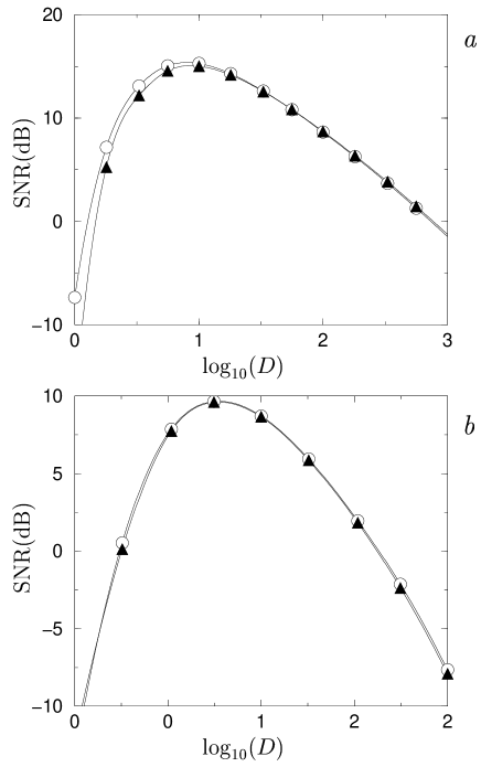
where is Gaussian white noise with zero mean, and correlation function . Here, small means that the effects of the nonlinear term are not large enough in order for the system to become bistable. The potential function giving the dynamics of the system is depicted in Fig. 1a, for different values of the resistance. In Fig. 2a we have shown the behavior of the SNR as a function of the noise level for two frequencies. The values of the remaining parameters are the same as the corresponding ones to the potential function of Fig. 1a. This figure clearly exhibits a maximum in the SNR.
When the nonlinear term is large enough, the system may display bistability. One state corresponds to all neurons at rest and the other to active neurons.
In Fig. 3a we have displayed the potential function associated to the Eq. (44), when the resistance varies for values of the parameters corresponding to the bistable situation. Note that when the resistance depends on time, the position of the minimum corresponding to the active state also changes periodically in time.
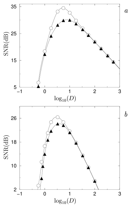
In order to analyze this situation, we have numerically integrated the corresponding equations as in the previous situation where the potential function is monostable. Fig. 4a displays the SNR which exhibits a maximum at a nonzero noise level.
In view to illustrate how the system behaves, in Fig. 5a we have shown three time series for different noise levels. This figure clearly manifests the presence of an optimum noise level, at which the response of the system is enhanced, and the displacement of the minima corresponding to active neurons.
IV Variation of the threshold
In the previous analysis we have studied the case in which the resistance of the neuron undergoes oscillations. Another possibility of temporal variation are oscillations in the parameter . Explicitly, the dynamics corresponding to this situation is described again by Eq. (10), but now and . By using the same assumptions about the parameters , , , and the gain introduced previously, we will now proceed in a similar fashion.
It is easy to see that in this case does not depend on time:
| (45) |
and the correction to the probability density due to the nonlinear term is given by
| (47) | |||||
The averaged value of is then
| (48) |
Note that for symmetry reasons, the integral in Eq. (47) gives a null contribution to . By expanding in the parameter around its zero value, we then obtain Eq. (33). In this case the susceptibility reads
| (49) |
The noise term is the same as in the previous case, then we obtain the following expressions for the signal, noise and SNR
| (50) | |||||
| (51) | |||||
| SNR | (52) |
This last expression clearly shows that the SNR has a maximum at a non-zero noise level then making the presence of SR manifest.
As we did in the previous situation, to study the case in which the oscillations and the nonlinear term are not infinitesimal, we have numerically solved the corresponding Langevin equation by using the procedure outlined above. In this case it reads
| (53) |
where is the same noise as the one defined previously. The explicit situation we have considered is given through the potential function displayed in Fig. 1b. In Fig. 2b we have shown the behavior of the SNR as a function of the noise level for two frequencies. The values of the remaining parameters are the same as those corresponding to the potential function of Fig. 1b. In this case the SNR also exhibits a maximum for the two frequencies.
Bistability may also be present in this case. In Fig. 3b we have represented the potential function when periodic modulations act through the threshold, for values of the parameters corresponding to the bistable situation. In contrast with the case of oscillations of the resistance, in which the minimum corresponding to the active state varies its position, when the threshold oscillates, the two minima always remain at the same transmenbrane potential.
This situation can also be analyzed through numerical integration. Fig. 4b displays the SNR for the periodic modulation we are considering. This quantity exhibits a maximum for the two frequencies. Finally, in Fig 5b we have also shown three time series for different noise levels. It is worth emphasizing that, for noise levels close to the optimum value, the time series look as those corresponding to the usual bistable quartic potential [3, 5].
V Discussion
In this paper we have analyzed how noise affects the behavior of a neural medium when it is periodically modulated. We have found that the occurrence of noise may play a constructive role since an optimized amount of it may contribute to enhancing the response of the system. Under some circumstances, the presence of noise is responsible for the appearance of oscillations which otherwise would not be manifested. In this regard, the analysis of macroscopic neural dynamics obtained from electroencephalograms has been a matter of debate over the last decade [40]. It is accepted that the activity of the brain cortex shows low-dimensional traits, though the exact nature of the phenomenon itself is far from being clear. Here we have shown that noise, sometimes not considered, could give rise to a coherent behavior of the system, then playing an important role in neural dynamics.
The mean field model we have proposed, although constituting an oversimplified picture of a thalamo-cortical network, might be a first step in our understanding of how noise and nonlinearities can generate interesting macroscopic outcomes. Further developments must include spatial effects as well as the consideration of activatory and inhibitory populations of neurons.
On what concerns to the phenomenon of SR itself, an important aspect that should be emphasized is the fact that the model we have presented exhibits SR in both monostable and bistable situations, depending on the values of the parameters. This remarkable feature contrasts with previous studies for which SR has been found only for monostable or bistable systems. Moreover, some bistable systems undergoing SR may become monostable, but under this circumstance SR does not take place. In fact, the model under consideration describes a system with a threshold, accounting for the firing of the neurons that may behave as a monostable or a bistable system. Therefore, we have envisaged a model that may exhibit three different situations (monostable, bistable, and threshold) where the phenomenon occurs.
Acknowledgments
This work was supported by DGICYT of the Spanish Government under Grants Nos. PB95-0881 and PB94-1195. J. M. G. V. wishes to thank Generalitat de Catalunya for financial support.
REFERENCES
- [1] R. Benzi, A. Sutera, and A. Vulpiani, J. Phys. A 14, L453 (1981).
- [2] S. Fauve and F. Heslot, Phys. Lett. A 97, 5 (1983).
- [3] B. McNamara, K. Wiesenfeld, and R. Roy, Phys. Rev. Lett. 60, 2626 (1988).
- [4] L. Gammaitoni, F. Marchesoni, E. Menichella-Saetta, and S. Santuchi, Phys. Rev. Lett. 62, 2626 (1989).
- [5] B. McNamara and K. Wiesenfeld, Phys. Rev. A 39, 4854 (1989).
- [6] A. Longtin, A. Bulsara, and F. Moss, Phys. Rev. Lett. 67, 656 (1991).
- [7] F. Moss, A. Bulsara, and M. F. Shlesinger (eds.), Proceedings of the NATO Advanced Research Workshop on Stochastic Resonance, San Diego, 1992 [J. Stat. Phys. 70, 1 (1993)].
- [8] J. K. Douglass, L. Wilkens, E. Pantazelou, and F. Moss, Nature 365 337 (1993).
- [9] F. Moss, in Some Problems in Statistical Physics, edited by G. H. Weiss (SIAM, Philadelphia,1994).
- [10] K. Wiesenfeld, D. Pierson, E. Pantazelou, C. Dames, and F. Moss, Phys. Rev. Lett. 72, 2125 (1994).
- [11] K. Wiesenfeld and F. Moss, Nature 373, 33 (1995).
- [12] J. F. Lindner, B. K. Meadows, W. L. Ditto, M. E. Inchiosa, and A. R. Bulsara, Phys. Rev. Lett. 75, 3 (1995).
- [13] Z. Gingl, L. B. Kiss, and F. Moss, Europhys. Lett. 29, 191 (1995).
- [14] M. Grifoni and P. Hanggi, Phys. Rev. Lett. 76, 1611 (1996).
- [15] F. Marchesoni, L. Gammaitoni, and A. R. Bulsara, Phys. Rev. Lett. 76 2609 (1996).
- [16] J. M. G. Vilar and J. M. Rubí, Phys. Rev. Lett. 78, 2886 (1997).
- [17] J. M. G. Vilar and J. M. Rubí, Phys. Rev. Lett. 78, 2882 (1997).
- [18] J. M. G. Vilar and J. M. Rubí, Phys. Rev. Lett. 77, 2863 (1996).
- [19] F. Chapeau-Blondeau and X. Godivier, Phys. Rev. E 55, 1748 (1997).
- [20] S. M. Bezrukov and I. Vodyanoy, Nature 385, 33 (1997).
- [21] A. Bulsara et al., Biol. Cybernet. 61, 211 (1989);
- [22] A. Bulsara et al., J. Theor. Biol. 152, 531 (1991).
- [23] M. Riani and E. Simonotto, Phys. Rev. Lett. 72, 3120 (1994).
- [24] J. J. Collins et al., Nature (London) 376, 236 (1995).
- [25] P. Jung and G. Mayer-Kress, Phys. Rev. Lett. 74, 2130 (1995).
- [26] A. Longtin et al., Phys. Rev. Lett. 67, 656 (1991).
- [27] D. R. Chialvo and A. V. Apkarian, J. Stat. Phys. 70, 375 (1993).
- [28] B. J. Gluckman et al., Phys. Rev. Lett. 77, 4098 (1996).
- [29] S.J. Schiff, K. Jerger, D.H. Duang, T. Chang, M.L. Spano and W.L. Ditto, Nature 370, 615 (1994).
- [30] D. Ferster, Science 273, 1812 (1996).
- [31] E. R. Kandel, J. H. Schwartz and T. M. Jessell, Principles of Neural Science (Prentice Hall, London, 1991).
- [32] For a review of recent literature see: A. Destexhe and A. Babloyantz, Neural Comp. 3, 145 (1991).
- [33] H. C. Tuckwell, Introduction to theoretical neurobiology, vol.2 (Cambridge U. Press, Cambridge, 1988).
- [34] G. M. Shepherd (ed.), The synaptic organization of the brain, 3rd edition ( Oxford U. Press, New York, 1990).
- [35] W. D. Knowles, R. D. Tranb, R. K. S. Wong, and R. Miles. Trends in Neurosci., February 1985, 73.
- [36] H. G. Schuster (ed.), Nonlinear dynamics and neuronal networks (Springer, Berlin, 1991).
- [37] J. D. Cowan and G. B. Ementrout, in Studies in Mathematical Biology, Part I, edited by S. A. Levin (The Mathematical Association of America, Washington, 1978).
- [38] P. E. Kloeden and R. A. Pearson, J. Austral. Math. Soc., Ser B, 20 8-12 (1977).
- [39] J. R. Klauder and W. P. Petersen, SIAM J. Numer. Anal. 22 1153-1166 (1985).
- [40] E. Basar (ed.), Chaos in Brain function (Springer, Berlin, 1990).