[

Ordering Periodic Spatial Structures by Noise

Abstract

We have analyzed the interplay between noise and periodic spatial modulations in bistable systems outside equilibrium and found that noise is able to increase the spatial order of the system, giving rise to periodic patterns which otherwise look random. This new phenomenon, which may be viewed as the spatial counterpart of stochastic resonance, then shows a constructive role of noise in spatially extended systems, not considered up to now.

]

Contrarily to intuitive arguments, arising from the frequent identification of noise with a source of disorder, in systems outside equilibrium the presence of noise may be responsible for an increase of order. Noise then can play a constructive role, losing its usually assumed character of nuisance. One of the most important manifestations of this constructive role played by noise takes place when noise and a weak signal periodic in time exhibit a cooperative behavior, giving rise to the enhancement of the periodic response. This fact, which is evidenced by an increase of the output signal-to-noise ratio (SNR) as the noise level increases, constitutes the main fingerprint of the phenomenon known as stochastic resonance (SR) [1, 2]. The importance and interest of SR has been revealed by the great number of situations in which it has been found [3, 4, 5, 6, 7, 8, 9, 10]. In regards to spatially extended systems, this constructive role of noise has only been reported for situations in which also a time periodic signal enters the system. This feature occurring in the phenomenon known as spatiotemporal stochastic resonance [11, 12, 13, 14, 15] only deals with the effects of the spatial degrees of freedom in the time evolution of the system, but no enhancement of the spatial order, in a similar fashion as the temporal order, has been found up to now.

In this Letter we show that randomness may be responsible for spatial ordering of a system in such a way that the emergent structures look more regular, i. e. periodic, when the noise level is increased. This new phenomenon can be viewed as the spatial counterpart of SR. In it, the SNR is defined through the structure factor instead of the power spectrum and the system is periodically modulated in space instead of in time. In this sense, noise is able to increase the order of a spatial structure in a similar fashion as noise is able to do it in the time evolution.

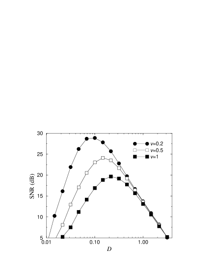
FIG. 1.: SNR as a function of the noise level for different values of the advection velocity: $v=0.2$, $0.5$, and $1$. The values of the remaining parameters are $r=1$, $g=1$, $\sigma=0.03$, $A=0.3$, and $k_{0}/2\pi=0.05$.

FIG. 2.: Structure factor as a function of the dimensionless wavenumber $kL/2\pi$, with $L$ ($=1024$) the length of the system, for three noise levels: $D=0.02$, $0.1$, and $1$ (from left to right). The values of the remaining parameters are $v=0.2$, $r=1$, $g=1$, $\sigma=0.03$, $A=0.3$, and $k_{0}L/2\pi=50$.

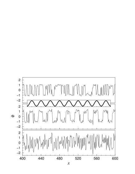
FIG. 3.: Field $\phi$ as function of position $x$ for the same situation as in Fig. 2 [$D=0.02$, $0.1$, and $1$ (from top to bottom)]. The inset illustrates the periodicity of the force which accounts for the spatial modulation.

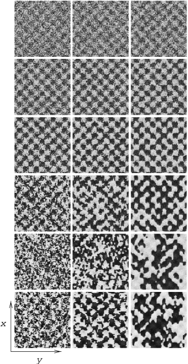
FIG. 4.: Representation of the two-dimensional field $\phi$ for different values of the noise level [$D=10^{-6/3}$, $10^{-5/3}$, $10^{-4/3}$, $10^{-3/3}$, $10^{-2/3}$, and $10^{-1/3}$ (from bottom to top)] and diffusion [$\sigma=10^{-9/6}$, $10^{-7/6}$, and $10^{-5/6}$ (from left to right)]. The system size is $100\times 100$. The values of the remaining parameters are $v=0.2$, $r=1$, $g=1$, $A=0.3$, and $k_{0}/2\pi=0.05$. Black and white colors stand for minimum and maximum values, respectively.

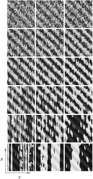
FIG. 5.: Representation of the two-dimensional field $\phi$ for different values of the disorder intensity [$D=10^{-6/3}$, $10^{-5/3}$, $10^{-4/3}$, $10^{-3/3}$, $10^{-2/3}$, and $10^{-1/3}$ (from bottom to top)] and diffusion [$\sigma=10^{-9/6}$, $10^{-7/6}$, and $10^{-5/6}$ (from left to right)]. The system size is $100\times 100$. The values of the remaining parameters are $v=0.5$, $r=1$, $g=1$, $A=0.3$, and $k_{0}/2\pi=0.03$. Black and white colors stand for minimum and maximum values, respectively.

To illustrate the essentials of the phenomenon we consider explicitly the $\phi^{4}$ model, although similar results could also be obtained for other systems provided that they exhibit bistability. Additionally, the system is under the influence of a spatial periodic force and driven outside equilibrium by advection. We first study the one-dimensional case in which the field $\phi$ is advected by a constant velocity $v$,

$$\partial_{t}\phi+v\partial_{x}\phi = r\phi-g\phi^{3}+\sigma\partial_{xx}\phi$$ (2)

$$+A\cos(k_{0}x)+\zeta(x,t)\;\;.$$

Here $A\cos(k_{0}x)$ is the periodic force, accounting for the spatial modulation, with $A$ the amplitude and $2\pi/k_{0}$ the period. The parameters $r$, $g$ and $\sigma$ are positive constants, whereas the noise term $\zeta(r,t)$ is Gaussian and white with zero mean and correlation function $\left<\zeta(x,t)\zeta(x^{\prime},t^{\prime})\right>=2D\delta(x-x^{\prime})\delta(t-t^{\prime})$, defining the noise level $D$.

With the purpose of characterizing the spatial configuration we will consider the structure factor defined as

$$F(k)=\left\langle\hat{\phi}_{k}\hat{\phi}_{-k}\right\rangle\;\;,$$ (3)

where $\hat{\phi}_{k}$ is the Fourier transform of the field $\phi(x)$ and $\langle\;\rangle$ indicates average over the noise realization. Due to the presence of the periodic force, it consists of a delta function centered at the wavenumber $k_{0}$ plus a function $Q(k)$ which is smooth in the neighborhood of $k_{0}$ and is given by

$$F(k)=Q(k)+S(k_{0})\delta(k-k_{0})\;\;.$$ (4)

The structure factor, as expressed previously, explicitly shows the intensity of the periodic component of the system, $S(k_{0})$, and the stochastic component, $Q(k)$. The SNR, defined as the ratio between both quantities,

$$\mbox{SNR}=S(k_{0})/Q(k_{0})\;,$$ (5)

then indicates the order present in the system.

To proceed further we have numerically integrated the previous equations by discretizing them on a mesh [16] and then by using standard methods for stochastic differential equations [17]. In Fig. 1 we have represented the SNR as a function of the noise level for representative values of the parameters corresponding to the bistable situation. This figure indicates, through the maximum of the SNR at a nonzero noise level, that the presence of an optimum amount of noise enhances the underlying periodic structure of the system. In this regard, in Fig. 2 we display the structure factor for the optimum, a higher and a lower noise level. The existence of a periodic pattern is revealed by the peak arising over the background noise at $k_{0}$, which for the optimum noise intensity, is more than an order of magnitude higher than for the other displayed intensities. An instance of how the enhancement of this peak, quantified by the SNR, manifest in the spatial structure is shown in Fig. 3. It is worth emphasizing the fact that the pattern for the optimum noise intensity looks more deterministic, i. e. periodic, than for lower noise intensities. In this regard noise constitutes a source of order. Further increasing of the noise level, however, destroys the coherent response to the periodic spatial modulation.

From Fig. 3 one can elucidate the mechanism giving rise to the enhancement of the structure. For the previous values of the parameters the system exhibits local bistability. The effect of the periodic force is then to spatially modulate the system in such a way that the most stable state changes from positive to negative values of the field $\phi$, depending on position. Since the field $\phi$ is advected, the system is unable to switch between these two states when noise level is too small. The presence of an optimum amount of noise, however, makes these transitions possible in a coherent fashion, giving rise to the enhancement of the underlying pattern. Further increasing the noise level completely destroys the coherent response. In this context, this mechanism is the spatial counterpart of the corresponding one of SR. Thereby, the parameter $vk_{0}$, which has dimensions of the inverse of time, plays the same role as the frequency $\omega_{0}$ in SR. This fact is displayed in Fig. 1, where the dependence of the SNR on $v$, for fixed $k_{0}$, is close to that on $\omega_{0}$ in the case of SR. The striking similarity with the temporal case is evidenced even more when considering Fig. 3 for the optimum noise level, which looks quite similar to a bistable system in time when exhibiting SR.

To illustrate more the fact that noise may imply ordering in nonequilibrium systems we have considered the two-dimensional counterpart of Eq. (2) on the $(x,y)$-plane. The periodic force is now $A\cos(k_{0}x)\cos(k_{0}y)$, whereas the system is again advected in the $x$-direction by a constant velocity $v$. The other terms follow by the straightforward extension to two dimensions. Hence, the system is described by

$$\partial_{t}\phi+v\partial_{x}\phi = r\phi-g\phi^{3}+\sigma\left(\partial_{xx}+\partial_{yy}\right)\phi$$ (7)

$$+A\cos(k_{0}x)\cos(k_{0}y)+\zeta(x,y,t)\;\;.$$

In Fig. 4 we have represented the field $\phi(x,y)$ obtained from numerical simulations for representative values of the parameters. For low and high noise level the spatial pattern is completely disordered. In contrast, an optimum nonzero amount of noise makes the presence of the underlying checkerboard pattern manifest. In this regard, the addition of noise is able to increase the order of the system giving rise to periodic structures which otherwise would not be observed. Notice that the periodicity in the perpendicular direction to the advection is also enhanced. It its worth emphasizing that, in contrast to the one-dimensional case, in two dimensions a temporal counterpart does not exist due to the one-dimensional character of time.

Another interesting situation comes when dealing with disorder represented by quenched noise [18]. The noise term is Gaussian with zero mean, but now with correlation function $\left<\xi(x,y)\xi(x^{\prime},y^{\prime})\right>=2D\delta(x-x^{\prime})\delta(y-y^{\prime})$. In this case, $D$ accounts for the degree of disorder. The explicit case we will study is

$$\partial_{t}\phi+v\partial_{x}\phi = r\phi-g\phi^{3}+\sigma\left(\partial_{xx}+\partial_{yy}\right)\phi$$ (9)

$$+A\cos[k_{0}(x+y)]+\zeta(x,y)\;\;,$$

where, for the sake of generality, we have considered a new expression for the periodic force. The effects of disorder are illustrated in Fig. 5 which displays the field $\phi(x,y)$ for representative values of the parameters. In the figure one can see that for weak disorder, i.e. low $D$, the pattern is quite random, although the direction of the advection is manifested in the elongated form of the spots. When increasing the disorder, the system is able to increase its order, then displaying periodic striped patterns. This constructive aspect, however, is lost by further increasing the intensity of the quenched noise. In this sense, there exists an optimum amount of disorder which is responsible for order.

It its worth pointing out that the phenomenon we have found is even more general than previously presented, since this kind of spatial ordering may also appear when advection is not present and even in systems without intrinsic spatial structure. For instance, by only replacing $x$ by $x-vt$ in Eq. (2) the advective term disappears and the force $A\cos(k_{0}x)$ becomes $A\cos[k_{0}(x-vt)]$. Under these circumstances, Eq. (2) describes the propagation of a plane traveling wave in a bistable medium. Thereby, the results we have obtained also apply to this case.

In summary, we have found a new phenomenon in which randomness is responsible for the spatial ordering of a system. In this regard, the addition of noise makes the presence of spatial periodicity manifest, giving rise, for instance, to checkerboard and striped patterns. We have shown the occurrence of the phenomenon for different types of spatial modulations and different types of randomness, such as white noise and spatial disorder. It is worth emphasizing that although our analysis has been explicitly carried out for the $\phi^{4}$ model, similar results could also be obtained for other systems provided that they exhibit bistability. Our findings, then, contribute to a wider understanding of the role of nonequilibrium fluctuations in spatially extended systems, indicating that this constructive aspect of noise, reported before only for temporal signals, is more universal than believed.

This work was supported by DGICYT of the Spanish Government under Grant No. PB95-0881. J.M.G.V. wishes to thank Generalitat de Catalunya for financial support.

REFERENCES

- [1] R. Benzi, A. Sutera, and A. Vulpiani, J. Phys. A 14, L453 (1981).
- [2] F. Moss, in Some Problems in Statistical Physics, edited by G. H. Weiss (SIAM, Philadelphia,1994).
- [3] B. McNamara, K. Wiesenfeld, and R. Roy, Phys. Rev. Lett. 60, 2626-2629 (1988);
- [4] B. McNamara and K. Wiesenfeld, Phys. Rev. A 39, 4854 (1989).
- [5] Proceedings of the NATO Advanced Research Workshop on Stochastic Resonance, San Diego, 1992 [J. Stat. Phys. 70, 1 (1993)].
- [6] K. Wiesenfeld, D. Pierson, E. Pantazelou, C. Dames, and F. Moss, Phys. Rev. Lett. 72, 2125 (1994).
- [7] K. Wiesenfeld and F. Moss, Nature 373, 33 (1995).
- [8] Z. Gingl, L. B. Kiss, and F. Moss, Europhys. Lett. 29 191-196 (1995).
- [9] A. Bulsara and L. Gammaitoni, Phys. Today 49, No. 3, 39 (1996).
- [10] J. M. G. Vilar and J. M. Rubí, Phys. Rev. Lett. 77, 2863 (1996).
- [11] P. Jung and G. Mayer-Kress, Phys. Rev. Lett. 74, 2130 (1995).
- [12] J. F. Lindner, B. K. Meadows, W. L. Ditto, M. E. Inchiosa, and A. R. Bulsara, Phys. Rev. Lett. 75, 3 (1995).
- [13] F. Marchesoni, L. Gammaitoni, and A. R. Bulsara, Phys. Rev. Lett. 76, 2609 (1996).
- [14] M. Löcher, G. A. Johnson, and E. R. Hunt, Phys. Rev. Lett. 77, 4698 (1996).
- [15] J. M. G. Vilar and J. M. Rubí, Phys. Rev. Lett. 78, 2886 (1997).
- [16] W.H. Press, B. P. Flannery, S. A. Teukolsky, and W. T. Vetterling, Numerical Recipes (Cambridge University Press, New York, 1986).
- [17] P. E. Kloeden and E. Platen, Numerical Solution of Stochastic Differential Equations (Springer-Verlag, Berlin, 1995).
- [18] It has been found that, paradoxically, the introduction of disorder may force a chaotic system to exhibit a periodic behavior in time [Y. Braiman, J. Lindner, and W. Ditto, Nature, 378, 465 (1995)]. However, in such a situation the spatial structure still remains disordered.