Crossover from Regular to Chaotic Behavior in the Conductance of Periodic Quantum Chains

Abstract

The conductance of a waveguide containing finite number of periodically placed identical point-like impurities is investigated. It has been calculated as a function of both the impurity strength and the number of impurities using the Landauer-Büttiker formula. In the case of few impurities the conductance is proportional to the number of the open channels $N$ of the empty waveguide and shows a regular staircase like behavior with step heights $\approx 2e^{2}/h$. For large number of impurities the influence of the band structure of the infinite periodic chain can be observed and the conductance is approximately the number of energy bands (smaller than $N$) times the universal constant $2e^{2}/h$. This lower value is reached exponentially with increasing number of impurities. As the strength of the impurity is increased the system passes from integrable to quantum-chaotic. The conductance, in units of $2e^{2}/h$, changes from $N$ corresponding to the empty waveguide to $\sim N/2$ corresponding to chaotic or disordered system. It turnes out, that the conductance can be expressed as $(1-c/2)N$ where the parameter $0<c<1$ measures the chaoticity of the system.

In recent years transport in a wide variety of mesoscopic systems has been investigated. One of the interesting questions is the behavior of the conductance of disordered identical blocks coupled in chain. This problem may arise whenever identical chaotic or disordered nanostructures are organized in a sequentially built structure. So far mostly chains with completely disordered/chaotic blocks have been studied[1, 2]. Our aim in this letter is to study a system in which chaoticity of the blocks can be tuned by varying a single parameter $c$ ranging from zero (completely regular) to one (completely chaotic). Well known examples of such systems are provided by point-like impurities with variable strength placed in regular waveguides[4, 5]. We study here the low temperature conductance of a waveguide containing finite number of periodically placed identical point-like impurities. In this model the conductance depends on the strength and on the number of impurities. It will be shown that when passing from the regular toward the quantum-chaotic case by increasing the impurity strength the average conductance (in units of $2e^{2}/h$) behaves like $\sim\alpha N$, where $\alpha=1-c/2$, interpolating between the conductance of the regular (empty) waveguide $N$ and the universal conductance of chaotic systems $\sim N/2$ determined by Random Matrix Theory[3] (RMT). The direct universal link between $c$, characterizing the chaoticity, and the average conductance is our main result.

We consider an ideal 2D waveguide of width $W$ which is divided into $L$ blocks of length $a$. We place an impurity with Dirac-delta potential $U(r)=\lambda\delta(r-r_{0})$ in each block, where $r_{0}$ is its position within a block (see Fig. 1) and $\lambda$ is the strength of the potential. Inside the block the potential is assumed to be zero and the wave functions should fulfill Dirichlet boundary condition ($\psi=0$) on the walls of the waveguide. The system is adiabatically matched to 2D electron reservoirs on both ends.

The conductance is given by the Landauer-Büttiker formula[6]

$$G(E_{F})=\frac{2e^{2}}{h}T,$$ (1)

where $T$ is the total transmission coefficient of the system at Fermi energy $E_{F}$. The total transmission can be expressed in terms of the partial transmission amplitudes $t_{nm}$ of open modes between the entrance and the exit of the waveguide

$$T=\sum_{n,m}|t_{nm}|^{2},$$ (2)

where the transmission amplitudes can be calculated from the retarded Green-function of the system[7]

$$t_{nm}=2i(k_{n}k_{m})^{1/2}\int dydy^{\prime}\Phi_{n}(y)G^{+}(x,y|x^{\prime},y^{\prime})\Phi_{m}(y^{\prime}).$$ (3)

Here $\Phi_{n}(y)=\sqrt{\frac{2}{W}}\sin(\pi ny/W)$ is the transverse part of the wavefunction of the empty waveguide

$$\psi_{n}(x,y)=\Phi_{n}(y)e^{ik_{n}x},$$ (4)

where $k_{n}=\sqrt{2mE_{F}-(\hbar\pi n/W)^{2}}$ for mode index $n$, $y$ is the transverse coordinate and longitudinal coordinates $x$ and $x^{\prime}$ lie anywhere on the entrance (left hand side in Fig. 1) and exit sides, respectively. The mode $n$ is open if $E_{F}>(\hbar\pi n/W)^{2}/2m$.

The retarded Green-function can be calculated recursively [8]. Adding a new impurity to a system with $L$ impurities changes the Green-function the following way

$$G^{+}_{L+1}(x,y|x^{\prime},y^{\prime})=G^{+}_{L}(x,y|x^{\prime},y^{\prime})+\tilde{\lambda}\frac{G^{+}_{L}(x,y|x_{0},y_{0})G^{+}_{L}(x_{0},y_{0}|x^{\prime},y^{\prime})}{1-\tilde{\lambda}G^{+}_{L}(x_{0},y_{0}|x_{0},y_{0})},$$ (5)

where the strength $\tilde{\lambda}$ should be renormalized

$$\tilde{\lambda}=\frac{\lambda}{1+\lambda G^{+}_{L}(x_{0},y_{0}|x_{0},y_{0},-E_{F})},$$ (6)

in order to make the calculations with the delta potential well defined [9]. The recursion starts with the retarded Green-function of the empty waveguide

$$G^{+}_{0}(x,y|x^{\prime},y^{\prime},E_{F})=\sum_{n=1}^{n_{max}}\frac{\Phi_{n}(y)\Phi_{n}(y^{\prime})}{2ik_{n}}e^{ik_{n}|x-x^{\prime}|},$$ (7)

where $n_{max}\rightarrow\infty$. In numerical calculation $n_{max}$ should be much larger than the number of open modes $N=Int(k_{F}W/\pi\hbar)$.

First we study the behavior of the conductance of the system with increasing number of blocks $L$ each containing one impurity of fixed strength $\lambda$. For the empty ideal waveguide ($L=0$) the transmission as a function of the Fermi wavelength $k_{F}=\sqrt{2mE_{F}}/\hbar$ is an ideal staircase with steps $T=N$, where $N$ is the number of open modes. Adding one impurity ($L=1$) slightly modifies the staircase[10] and the transmission remains still close to $N$. By adding more impurities the staircase disappears and an irregular structure emerges as it is shown in the upper part of Fig. 2 (solid line) for $L=10$. The transmission for $L\rightarrow\infty$ at a fixed Fermi wavelength decreases toward an asymptotic value which is the transmission of the infinitely long periodic system.

The eigenmodes of the infinitely long periodic system are the Bloch functions

$$\psi_{q,n}(x,y)=e^{iqx}u_{q,n}(x,y),$$ (8)

where $u_{q,n}(x+a,y)=u_{q,n}(x,y)$ and $-\pi/a<q<\pi/a$ with eigenenergies $\epsilon_{n}(q)$ forming a band structure. In this case the transmission is given by the number of Bloch modes $N_{B}$ propagating in positive $x$ direction at Fermi energy $E_{F}$, which can be determined by counting the number of solutions $(n_{i},q_{i}),i=1,...,N_{B}$ for $q_{i}>0$ of

$$\epsilon_{n_{i}}(q_{i})=E_{F}.$$ (9)

In the lower part of Fig. 2 the band structure for a given value of $\lambda$ is shown for $q>0$. Here one can count the number of intersections of bands with $k_{F}$ yielding $N_{B}$ and the transmission $T=N_{B}$ of the infinite system is plotted on the upper part of Fig. 2 (dashed line). We can see that the transmission, even for $L=10$, approaches integer values corresponding to the transmission of the infinite system. The transmission drops to zero when $k_{F}$ is in a gap of the band structure and it jumps whenever $k_{F}$ is on the edge of a band.

Next we study the $L$ dependence of the average transmission $<T>_{N}$ corresponding to a fixed number of open modes $N$, i.e. for Fermi wavelengths from $k_{F}=N$ to $k_{F}=N+1$ (hereafter measured in units of $\pi\hbar/W$),

$$<T>_{N}=\int_{N}^{N+1}T(k_{F})dk_{F}.$$ (10)

In Fig. 3 $<T>_{10}$ is shown as a function of the number of blocks $L$ for different values of $\lambda$. The average transmission as the function of $L$ decreases exponentially and can be well approximated with the expression

$$<T>_{N}=(N-T_{\infty}(\lambda,N))e^{-L/\xi(\lambda,N)}+T_{\infty}(\lambda,N),$$ (11)

where $\xi$ characterizes the rate of decay and $T_{\infty}$ is the number of modes remaining open for $L\rightarrow\infty$. We can interpret $\xi$ as a partial localization length in the sense that the conductance decays exponentially with the size of the system, however it does not decay to zero, like in case of strong-localization, due to the periodicity of the system.

In Fig. 4 we plotted the asymptotic transmission $T_{\infty}$ as a function of the number of open modes $N$ for different values of $\lambda$. The transmission $T_{\infty}$ seems to scale approximately linearly with $N$. For large $\lambda$ it is in good agreement with the prediction of the Circular Orthogonal Ensemble (COE) of RMT for large N

$$T_{COE}\approx\frac{N}{2}-\frac{1}{4},$$ (12)

worked out for chaotic cavities with time reversal symmetry in Ref.[11]. For other values of $\lambda$ one can fit

$$T_{\infty}(\lambda,N)=\alpha(\lambda)N+\beta(\lambda).$$ (13)

In Fig. 5 the fitted parameters $\alpha(\lambda)$ and $\beta(\lambda)$ are shown. One can see that $\beta$ is approximately independent of $\lambda$ and takes the value $-1/4$, the weak localization correction, predicted by RMT. This means, that this weak localization correction sets in if back scattering is possible ($\lambda\neq 0$), however it does not depend on the details of its mechanism.

The parameter $\alpha$ decreases from $\alpha\approx 1$ to $\alpha\approx 1/2$ with increasing $\lambda$. The $\lambda$ dependence of $\alpha$ can be explained by making a simple assumption about the relation between the conductance and the chaoticity of the system as we are going to show next. The Hamiltonian in systems which are neither completely regular nor chaotic can be divided into a regular $H_{R}$ and a chaotic $H_{C}$ part

$$H=H_{R}+H_{C}.$$ (14)

In our case $H_{R}$ is the Hamiltonian of a block of the empty waveguide and $H_{C}$ is associated with the delta impurity in it. The regular part can be modeled with a diagonal matrix with random elements and mean level spacing $\Delta$. The chaotic part can be modeled with a random Gaussian matrix drawn from the suitable orthogonal ensemble (GOE, GUE etc.) reflecting the symmetry of the system. The variance of the elements of the random matrix should coincide with the variance of the matrix elements of the chaotic part of the Hamiltonian i.e. $\sigma^{2}=\overline{|<i|H_{C}|j>|^{2}}$. The energy level statistics of such systems is transitional between Poissonian and tpure RMT. The chaoticity of the system, reflected in the level statistics, is determined by the transition parameter $\eta=\pi\sigma/\Delta$ whose universality was shown in many applications[12]. The appropriate measure of the chaoticity of a system is the rescaled parameter defined in Ref.[13]

$$c=\frac{\eta}{\sqrt{1+\eta^{2}}}$$ (15)

ranging from $0$ to $1$. The value $c=0$ corresponds to a completely regular system (the empty waveguide) and for $c=1$ the system is completely chaotic ($\lambda\rightarrow\infty$) in a quantum-chaotic sense. Analogously, in our numerical calculation ($W=a=1$), the chaoticity parameter $c$ can be defined as

$$c(\lambda)=\frac{\lambda/4}{\sqrt{1+(\lambda/4)^{2}}}.$$ (16)

Using semiclassical considerations for large $N$ we can make connection between the chaoticity parameter $c$ and the parameter $\alpha$ characterizing $T_{\infty}$ for $N\rightarrow\infty$. Semiclassically a part of the trajectories is bouncing between the walls only, while the rest is scattered by the impurities irregularly. Accordingly, the transmission can be approximately partitioned into a regular and a chaotic part. We can assume that the effective number of chaotic modes is $N\cdot c$ while the number of regular modes is $N\cdot(1-c)$. For regular modes the propagation is ideal, free from reflection and their contribution to the transmission is $N\cdot(1-c)$. On the other hand, according to the RMT result (12), only half of the chaotic modes contribute to the transmission and we get

$$T_{\infty}\approx N\cdot(1-c)+\frac{1}{2}N\cdot c,$$ (17)

yielding

$$\alpha=1-c/2.$$ (18)

In Fig. 5 we compared the numerically fitted values of $\alpha(\lambda)$ (see Eq. (13)) to $1-c(\lambda)/2$ (see Eq. (16)) and we have found excellent agreement in the whole range $\lambda=1-500$ supporting our new formula (18).

We conjecture that our new formula (18) is valid for the transmission of a much broader class of systems. It is expected that it works for the transmission through a system, attached to leads, whose level statistics (without leads) is transitional[13] in between Poissonian and RMT and can be characterized with $0<c<1$, since the assumption made above are valid in this case too. This makes it possible to determine the chaoticity of a system from the relation

$$c=2\cdot(1-\alpha),$$ (19)

by estimating $\alpha$ from the conductance. We hope that further numerical and possible experimental studies will support the results presented here.

This work has been supported by the Hungarian Science Foundation OTKA (F019266/F17166/T17493) the Hungarian Ministry of Culture and Education FKFP 0159/1997 and the Hungarian-Israeli R&D collaboration project (OMFB-ISR 96/6). J. Cs. thanks the financial support of The Royal Society of London.

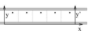
FIG. 1.: Schematic picture of the waveguide containing periodically placed impurities. The distance between the impurities is $a$ and the width of the guide is $W$. The entrance is on the left hand side. In the numerical calculations we choose $W=a=1$ and the position of the impurities was $x_{0}=0.65$ and $y_{0}=0.84$ with respect to the left lower corner of the unit cell.

FIG. 2.: In the upper part the transmission vs. the Fermi wavelength in units of $\hbar\pi/W$ is plotted for a system with $L=10$ blocks (solid line) and for an infinitely long system $L=\infty$ (dashed line). $\lambda=5$ in both cases. The rapid fluctuations of the conductance are on the scale $\Delta k\sim 1/La$ caused by the multiple scattering between the two ends of the device. In the lower part the band structure of the infinitely long system is plotted for the same parameter $\lambda$ as above. The vertical axis is the Bloch number $q$ and $k_{n}(q)=(2m\epsilon_{n}(q))^{1/2}/\hbar$ has been plotted in units of $\hbar\pi/W$. This representation makes it possible to get the transmission of the infinitely long system in the upper part from the bands of the lower part graphically.

FIG. 3.: The average transmission for $N=10$ open modes as a function of the number of blocks $L$ at different values of impurity strength $\lambda$ and for $W=a=1$. $<T>_{10}$ decreases from $10$ (the transmission of the empty waveguide) exponentially as a function of $L$ for all $\lambda$. Around $L\approx 50$ it reaches an asymptotic value depending on $\lambda$. For large $\lambda$ (chaotic case) this asymptotic value is close to $N/2=5$ predicted by Random Matrix Theory.

FIG. 4.: The asymptotic transmission $T_{\infty}$ as a function of the number of open modes $N$ of the empty waveguide for different values of $\lambda$ in the range of $1-500$. The solid line represents the COE result $T=N^{2}/(2N+1)$.

FIG. 5.: The parameters $\alpha$ and $\beta$ (see Eq. (13)) of the linear fit to the data of Fig. 4 for different values of $\lambda$ in the range of $1-500$. a, parameter $\alpha$ vs. $\lambda$ (diamonds) and our prediction $\alpha=1-c(\lambda)/2$ (see. Eq. (17)). The errorbars represent the error of the linear fit. b, parameter $\beta$ versus $\lambda$ (diamonds) and the weak localization correction $-1/4$ (solid line).

REFERENCES

- [1] N. Taniguchi and B. L. Altshuler, Phys. Rev. Lett. 71, 4031 (1993)
- [2] T. Dittrich, B. Mehlig, H. Schanz and U. Smilansky , Chaos Solitons & Fractals 8, 1205 (1997)
- [3] M. L. Mehta, Random Matrices and the Statistical Theory of Energy Levels, Academic Press, New York and London (1967)
- [4] A. Shudo, Y. Shimizu, P. Śeba, J. Stein, H-J. Stöckmann and K. Źyczkowski, Phys. Rev. E49, 3748 (1994)
- [5] P. Śeba, Phys. Rev. Lett. 64, 1855 (1990)
- [6] R. Landauer, Phyl. Mag. 21, 1761 (1970); M. Büttiker, Phys. Rev. Lett. 57, 1761 (1986)
- [7] H. Baranger and D. Stone, Phys. Rev. B40, 8169 (1991)
- [8] C. Grosche, Ann. der Physik 2 557 (1993)
- [9] C. Grosche, Ann. der Physik 3 283 (1994)
- [10] G. Vattay, J. Cserti, G. Palla and G. Szálka, Chaos, Solitons & Fractals 8, 1031 (1997)
- [11] H. Baranger and P. Mello, Europ. Lett. 33, 465 (1996)
- [12] A. Pandey and M. L. Mehta, J. Phys. A16, L601, 2655 (1983) J. B. French, V. K. B. Kota, A. Pandey and S. Tomsovic, Ann. Phys. (NY) 181, 198 (1988); T. Guhr and H. A. Weidemüller, Ann. Phys. (NY) 193, 472 (1989);
- [13] T. Guhr, Ann. Phys. (NY) 250, 145 (1996)