Abstract - In this paper we will give a short rewiew about the conductance of a mesoscopic waveguide strip with a few impurities. Green-function method is used allowing to treat systems with low number of impurities, not only the completly clean case. Investigating a wire containing Dirac-delta potentials (modelling the impurities) we found that increasing number of impurities can cause a transition of the structure of conductance. The staircase like structure of the clean system vanishes and the conductance of a system containing finite number of impurities located periodically will be determined by the band structure of the periodic system.

1 Introduction

In recent years mesoscopic [1] devices have been studyed intensively. Exact quantum mechanical calculations have been compared with short wavelength description of clean systems without impurity (ballastic regime), or with random matrix predictions for systems densely packed with impurities causing wild fluctuations of the potential on all length scales (diffusive regime). Nowadays thanks to the advances in manufacturing and material design one can get two dimensional electron gas in semiconductors whose behaviour is worth studying. These electrons can be considered as free electrons with effective mass. Using advanced nanotechnology waveguide strips with special geometry in extremely small size (50-500nm) can be produced. We investigated theoretically such kind of wire containing a few impurities (between 1 and 100) with the simpliest geometry we can imagine. (For one impurity see fig. 1.)

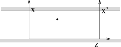
Figure 1: The lead with one impurity and the suitable coordinates

Investigating the conductance of this kind of systems experimentally gave a surprising result. In this kind of extremely small systems in pure metals the conductance is a staircase like function of the Fermi wavenumber, with steps of heights approximately $2e^{2}/h$. On Fig. 2, where this behaviour can be seen, we show our result for the system on Fig. 1. The explanation of this kind of behavior was given first by Landauer and B
”uttiker [2].

Figure 2: The conductance of the wire in case of one impurity in the universal units $2e^{2}/h$. The Fermi wavelength is plotted in units of $\pi/a$ where let $a$ denote the width of the wire. In this unit a new channel always opens at the integers.

Similar studies can be found in Ref. [4, 5, 6] for the case of one impurity modelled by Dirac-delta potential.

In this paper we first explain the Landauer formula which one may use for calculating the transmission or reflexion matrixelements of a system. Then in section “Green-function method” we give a short review of Green-function method which is very helpful treating systems containing low number of impurities. We then consider the conductance of a periodic system (see Fig. 3) and at the end of the last section we compare conductance calculated in section 3 with Green-function method and the one for the periodic case developed in section “Periodic case”.

2 Landauer formula

The conductance of the non-degenerate electron gas in a waveguide considered here is given by the Landauer formula [2, 3]. According to this theory, incoming and outgoing wave functions in the leads far from impurities can be decomposed into incoming and outgoing quantum modes

$$\psi_{n}(x,z) = \Phi_{n}(x)e^{ik_{n}z},$$

$$\Phi_{n}(x) = \sqrt{\frac{2}{a}}\sin(\frac{\pi nx}{a}),$$ (1)

where $k_{n}=\sqrt{2mE_{F}-(\hbar\pi n/a)^{2}}/\hbar$ is the wave number of the propagating planewave, $a$ is the width of the lead and $E_{F}$ is the Fermi energy. If the Fermi energy is less than $E_{n}=\frac{1}{2m}(\hbar\pi n/a)^{2}$ the wavenumber $k_{n}$ becomes imaginary and the $n^{th}$ channel becomes closed preventing wave propagation.

The Landauer formula for the conductance $G(E_{F})$ at Fermi energy $E_{F}$ is

$$G(E_{F})=\frac{2e^{2}}{h}\sum_{m,n}|t_{mn}|^{2},$$ (2)

where $t_{nm}$ is the transmission probability amplitude from the incoming channel $n$ on the entrance side to the outgoing channel $m$ on the exit side. In case of infinitely long leads summation goes for open channels of both sides only. The transmission probability is given by the projection of the Green-function over the transverse wave functions $\Phi_{n}(x)$ on the entrance lead for the incoming modes and $\Phi_{m}(x^{\prime})$ on the exit lead for outgoing modes

$$t_{nm}=2i(k_{n}k_{m})^{1/2}\int dxdx^{\prime}\Phi_{n}(x)G^{+}(r,r^{\prime},E)\Phi_{m}(x^{\prime}),$$ (3)

where $r,r^{\prime}$ denote the vector $(x,z),\,(x^{\prime},z^{\prime})$ and $z$, $z^{\prime}$ can lie anywhere on the entrance side and exit side, respectively. Reflection between two modes $n$ and $m$ on the same side is given by

$$r_{nm}=\delta_{nm}-2i(k_{n}k_{m})^{1/2}\int dxdx^{\prime}\Phi_{n}(x)G^{+}(r,r^{\prime},E)\Phi_{m}(x^{\prime}),$$ (4)

where $z$ lies anywhere on the entrance side. For open channels $n$ of the entrance side the transmission and reflection amplitudes fulfill the sum rules

$$\sum_{m}|t_{nm}|^{2}+\sum_{m^{\prime}}|r_{nm^{\prime}}|^{2}=1,$$ (5)

where the two summations go for channels $m$ on the exit side and $m^{\prime}$ on the entrance side. These are the consequences of the current conservation.

3 Green-function method

The Hamiltonian of the system with one impurity can be separated into two parts

$$\bf H=\bf H_{0}+\bf H_{1}.$$ (6)

where

$$\bf H_{0}=-{\Delta}$$ (7)

is the free particle Hamiltonian with effective mass $m$ of the electron and

$$\bf H_{1}(r^{\prime\prime})={\lambda}{\delta}(r^{\prime\prime}-r_{0})$$ (8)

models the potential of the impurity, (see Fig. 1.) using $\hbar=1,m=\frac{1}{2}$.

In order to study the case with impurity the Dyson equation can be used. It gives as the Green-function of the system we get adding a new potential (V) to a system whose Green-function is known $(G_{0})$

$$G(r,\,r^{\prime},\,E)^{+}=G_{0}^{+}(r,\,r^{\prime},\,E)+\int dr^{\prime\prime}G_{0}^{+}(r^{\prime},\,r^{\prime\prime},\,E){\bf V}(r^{\prime\prime})G^{+}(r,\,r^{\prime\prime},\,E).$$ (9)

If we know the Green-function of the empty waveguide strip ($G_{0}$) and we add one Dirac-delta potential at $r_{1}$ with the strength of $\lambda$, the Green-function of the wire with one impurity will be the following:

$$G^{+}(r,\,r^{\prime},\,E)=G_{0}^{+}(r,\,r^{\prime}\,E)+{\lambda}\frac{G_{0}^{+}(r,\,r_{1},\,E)G_{0}^{+}(r_{1},\,r^{\prime},\,E)}{1-{\lambda}G_{0}^{+}(r_{1},\,r_{1},\,E)}.$$ (10)

Including more impurities we can apply the Dyson equation more times for calculating the Green-function for this case [7].

In our method first the Green-function of the empty waveguide needs to be calculated. In our case this Green-function can be defined as

$$(E-{\bf H}_{0})G_{0}^{+}(r,\,r^{\prime},\,E)={\delta}(r-r^{\prime}).$$ (11)

The solution of this equation (11) is

$$G_{0}^{+}(r,\,r^{\prime},\,E)=\sum_{n}\frac{{\Phi}_{n}(x){\Phi}_{n}(x^{\prime})}{2ik_{n}}e^{ik_{n}\mbox{$\left|z-z^{\prime}\right|$}}\;.$$ (12)

where

$$k_{n}=\sqrt{E-\frac{n^{2}}{a^{2}}{\pi}^{2}}.$$ (13)

Once we know the Green-function using (3) the conductance can be developed. The results we can get using the tools developed here will be considered at the end of the next section.

4 Periodic case

In this section we calculate the electronic band structure of a periodic system, where each unit cell contains one impurity (see Fig. 3).

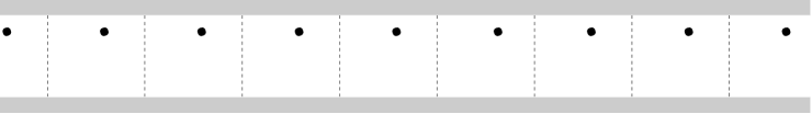
Figure 3: The periodic case, where the location of the impurity is x=0.86, z=0.65, the length of the blocks are 1 and the width of the lead, a is also 1.

Treating the periodic case we have the following Hamiltonian

$$\frac{{\hat{p}}^{2}}{2m}\Psi(x,z)+V(x,z)\Psi(x,y)=E\Psi(x,y).$$ (14)

It is wellknown that for periodic system the wavefunction can be given as

$$\Psi_{k,n}=e^{ikz}u_{k,n}(x,y),$$ (15)

where $u_{k,n}(x,z)$ is yet unknown function, and $k$ is a Bloch number. Inserting (15) into (14) we can obtain a new kind of Hamiltonian for the function of $u_{k,n}(x,z)$.

$$\frac{1}{2m}\bigg{(}\hbar k+\frac{\hbar}{i}\nabla\bigg{)}^{2}u_{k,n}(x,z)+V(x)u_{k,n}(x,z)=E_{k,n}u_{k,n}(x,y),$$ (16)

At the first step of the calculation, the Green-function of the empty system will be developed. In this case the $V(x,z)$ potential is zero, except the hard wall boundary of the wire, which corresponds to Dirichlet boundary condition. It is easy to obtain the solution that satisfies the equation (16), with the Dirichlet boundary condition.

$$u_{k,n}(x,z)=\sqrt{\frac{2}{a}}sin(\frac{n\pi x}{a}),\;\;\;n=1,2,...$$ (17)

Note that it does not depend on $z$. The eigen-energies of the empty wire are given then as

$$E_{k,n}=\frac{\hbar^{2}}{2m}\bigg{(}(k+K)^{2}+\frac{n^{2}\pi^{2}}{a^{2}}\bigg{)},$$ (18)

where $K=2\pi j/L$ belongs to the reciprocal lattice (L is the length of the unit cell, and j denotes any integer).The Green-function of the empty wire is

$$G_{0,k}(r,r^{\prime},E)=\frac{2}{a}{\sum_{K}}{\sum_{n}}\frac{\sin(\frac{n\pi x}{a})\sin(\frac{n\pi y}{a})}{E-E_{k,n}}.$$ (19)

Now using Dyson equation the Green-function of the system each block containing one Dirac-delta potential at $r_{0}$ with the strength $\lambda$ can be written as

$$G_{k}(r,r^{\prime},E)=G_{0,k}(r,r^{\prime},E)+\lambda\frac{G_{0,k}(r,r_{0},E)G_{0,k}(r_{0},r^{\prime},E)}{1-\lambda G_{0,k}(r_{0},r_{0},E)}.$$ (20)

In order to find the eigen-energies of this system with impurities, one has to find the singularities (poles) of the Green-function (20). A short calculation can show that the only singularity we have here comes from the denominator of the formula (20). Then the equation for the eigen-energies will be the following

$$0=1-\lambda G_{0,k}(r_{0},r_{0},E(k))\,,$$ (21)

which one has to solve and the eigen-energies ($E(k)$) can be calculated.

As soon as we have the band structure $(E(k))$ of the wire (Fig. 4. below), one may calculate the conductance of the periodic system. It is wellknown, that for calculating the conductance, the number of bands at a given energy level has to be counted. Each band gives a unit of ($2e^{2}/h$) to the conductance.

Figure 4: The bandstructure of the system (below) and the conductance of the periodic case calculated from the given bandstructure (above). The units as usuall.

Now let us use the results of the Green-function method (section 3). We have seen the conductance for the case of one single Dirac-delta. This case can be regarded as a block which contains the potential, connected to two extremely (infinitely) long empty wires. The periodic case can be built up from the same blocks. Now the next step is to connect two such

Figure 5: Low number of impurities in a lead. Each block are equivalent, however it is not the periodic case. In the blocks the location of the impurity is x=0.86, z=0.65, the length of the blocks are 1 and the width of the lead, a is also 1.

blocks, and then the two empty wires. We can go on with this iteration, we can connect any number of the same blocks and the two infinitely long wires. The case of four blocks can be seen on Fig. 5. Using Landauer formula and the Green-function method we can easily calculate the conductance of these systems. The results show a very interesting behaviour. If there are a few blocks in the wire (1-3) the staircase structure seen on Fig. 2 remains structurally unchanged with some deformation of the shapes of the steps. However inserting more impurities a new situation occurs. We can hardly see the reminescences of the structure of the Fig. 2, a new structure is developing. Once we compare this kind of conductances with the conductance calculated from the periodic system, we can see that between these two kinds of conductance, the difference is diminishing with increasing number of the inserted blocks (Fig. 6).

Figure 6: We can compare the two kind of conductance. The dotted line denotes the shape of the periodic case calculated from the given band structure (see also fig. 4). The continuos line denote the conductance of the system where 50 blocks where connected and also the two extremely long empty lead

.

5 Summary

In this paper a short review has been given about the transport behaviour of mesoscopic leads using Green-function theory. Thanks to the Dirac-delta potential an exact Green-function is available for the case of low number of impurities. As soon as the band structure is known, the conductance of the periodic case is also known. When the number of the impurities in the lead are increasing, the ideal staircase steps are deforming, and a new structure, determined by the band structure of the periodic system occurs.

6 Acknowledgments

We would like to thank S. Witoszynskyj the special opportunity to write this paper, P. Pollner, A. Csordás, T. Tasnádi, G. Tichy their interest, and encouragement. This work has been supported by the Hungarian Science Foundation OTKA (F019266/F17166/T17493), Hungarian Ministry of Culture and Education (FKFP0159/1997), and the Israeli-Hungarian collaboration grant (OMFB-ISR9/96).

References

- [1] C. W. Beenakker, H. van Houten in Solid State Physics, edited by H. Ehrenreich and D. Turnbull (Academic, New York, 1991), Vol. 44, pp. 1-228 4
- [2] R. Landauer, IBM J. Res. Dev. 1, 223 (1957); Phylos. Mag. 21, 863 (1970); M. Büttiker, Phys. Rev. Lett. 57, 1761 (1986)
- [3] H. Baranger and D. Stone, Phys. Rev. B40, 8169 (1989)
- [4] P. Bagwell, Phys. Rev. B41, 10354 (1990); A. Kumar, P. Bagwell, Phys. Rev. B43, 9012 (1991); S. Chaudhuri, S. Bandyopadhyay, M. Cahay, Phys. Rev. B45, 11126 (1992); Th. M. Nieuwenhuizen, A. Lagendijk, B. A. Tiggelen, Phys. Lett. A169, 191 (1992)
- [5] G. Vattay, J. Cserti, G. Palla, G. Szálka, Chaos, Solitons & Fractals, 8, 1031 (1997)
- [6] G. Palla, G. Szálka, Study Eötvös University, Budapest
- [7] C. Grosche, Ann Physik, 2, 557 (1993).
- [8] G. Vattay, G. Szálka and J. Cserti To be published