Identification of domain walls in coarsening systems at finite temperature

Abstract

Recently B. Derrida [Phys. Rev. E 55, 3705 (1997)] introduced a numerical technique that allows one to measure the fraction of persistent spins in a coarsening nonequilibrium system at finite temperature. In the present work we extend this method in a way that domain walls can be clearly identified. To this end we consider three replicas instead of two. As an application we measure the surface area of coarsening domains in the two-dimensional Ising model at finite temperature. We also discuss the question of to what extent the results depend on the algorithmic implementation.

I Introduction

Dynamical systems quenched from a disordered into an ordered phase may display interesting coarsening phenomena [1]. A simple example is the Ising model evolving by heat bath (HBD) or Glauber dynamics (GD). In the ordering phase of this model, starting with random initial conditions, patterns of ferromagnetic domains are formed whose typical size grows with time as $t^{1/2}$. For zero temperature, these domains are fully ordered and the domain walls evolving in time can be identified as bonds between oppositely oriented spins [2]. For nonzero temperature, however, it is hard to define domains and domain walls because it is difficult to distinguish between ‘true’ domains and minority islands generated by thermal fluctuations. This situation emerges, for example, in the two-dimensional ($2D$) Ising model at finite temperature below $T_{c}$ (see Fig. 1a).

Recently B. Derrida [3] proposed a method that allows one to measure properties related to coarsening in presence of thermal fluctuations. The main idea of this method lies in the comparision of two identical copies (replicas) $A$ and $B$ of the same system. Both replicas are submitted to the same thermal noise, i.e., their numerical updates are determined by the same sequence of random numbers. Copy $A$ starts with random initial conditions and begins to coarsen whereas copy $B$ starts from a fully magnetized state and therefore remains ordered as time evolves. The assumption is that all spin flips occurring in replica $B$ can be regarded as thermal fluctuations. Therefore, when a spin flip occurs simultaneously in both replicas, it can be considered as a thermal fluctuation, otherwise as a fluctuation due to the coarsening process.

In Refs. [3, 4] this method was used to determine the fraction of persistent spins [5] at nonzero temperature as a function of time. At zero temperature a spin is said to be persistent up to time $t$ if it never flipped before. In the Ising model the fraction of persistent spins $r(t)$ decays according to a power law $r(t)\sim t^{-\theta}$ where $\theta$ is an independent exponent. For the $1d$ Glauber model it was proved that $\theta=3/8$ [6] whereas in higher dimensions $\theta$ could only be determined by numerical simulations [5] and approximation methods [7]. For $T>0$, however, the fraction of spins that never flipped decays exponentially since thermal fluctuations occur everywhere at some finite rate. To overcome this difficulty, Derrida proposed to consider a spin as “persistent” if its temporal evolution in copies $A$ and $B$ is fully synchronized up to time $t$. Using this definition of persistence he analyzed the $2D$ Ising model and observed that $r(t)$ decays algebraically for $0\leq T\leq T_{c}$ and saturates at some finite value for $T>T_{c}$. Below the critical temperature the exponent $\theta$ seems to be the same as for $T=0$ while at $T=T_{c}$ a different exponent is observed.

An imperfection of the method developed by Derrida is that only one type of domain can be identified, namely, those that are magnetized in the same way as system $B$. Therefore different spin flips in $A$ and $B$ indicate the presence of oppositely magnetized domains rather than the presence of a domain wall. This means that persistent spins can be identified only in those domains which have the same orientation as copy $A$. For the same reason the method cannot be used to analyze other properties such as, for example, the dynamics of domain walls.

In the present work we extend Derrida’s method in a way that domain walls can be identified. For this purpose we consider three replicas $A,B,C$ instead of two. As before, all replicas are submitted to the same realization of noise. Replica $A$ starts with random initial conditions and serves as the master copy in which the coarsening process takes place. The temporal evolution of replica $A$ is compared with that of replicas $B$ and $C$, which start from fully ordered initial conditions with positive and negative magnetization, respectively. As in the original setup, domains with positive magnetization in copy $A$ exhibit the same thermal fluctuations as copy $B$. Likewise, thermal fluctuations in domains with negative magnetization in copy $A$ are synchronized with those in copy $C$. Along the domain walls, however, fluctuations in replica $A$ may occur that are different from those in $B$ as well as in $C$. Detecting such fluctuations by an appropriate observable (to be defined below) we are able to identify domain walls in a coarsening process at nonzero temperature. The remarkable efficiency of this method is illustrated in Fig. 1b. In addition, our technique allows one to measure interesting physical quantities such as, for example, the surface area of domains as a function of time. In what follows we restrict ourselves to the $2D$ Ising model evolving by HBD and GD. However, the technique can easily be generalized and may be applied to many other stochastic coarsening processes. For example, applying the method to the Potts model with $q>2$ states per site requires introducing $q+1$ different replicas.

A fundamental problem of numerical methods based on several replicas evolving under the same noise is that the results may depend on the algorithmic implementation. This was first observed in so-called damage spreading (DS) problems. In DS simulations [8] two replicas of a nonequilibrium system, submitted to the same thermal noise, are started from slightly different initial conditions. If the difference between the two copies (the damage) stays finite or even diverges, the system is said to exhibit damage spreading. Otherwise, if the two replicas merge into a fully synchronized evolution, damage is said to heal. Initially DS fascinated researchers, since it would have indicated the existence of different dynamical phases in stochastic models analogous to chaotic and regular phases in deterministic systems. However, later it was realized [9] that such DS phases are ambiguous since the usage of different but equivalent algorithms for the same dynamical system can lead to different DS phase structures [10]. For example, in the Ising model with HBD damage always heals while in the case of GD damage may spread [11]. The reason is that GD and HBD, although indistinguishable on a single replica, are characterized by different correlations when two or more replicas are simulated using the same random numbers [12]. As we are going to demonstrate, a similar algorithmic dependence appears in the present numerical technique where several replicas submitted to the same noise are used to analyze coarsening processes. Thus we have to verify to what extent the results obtained by Derrida [3] in the case of HBD  are physically relevant or rather artifacts of different algorithmic schemes.

The article is organized in the following way. In Sec. II we define HBD and GD as well as an observable by which domain walls can be detected. Our numerical results for HBD are presented in Sec. III. By comparing results for HBD and GD, we address the problem of algorithmic independence in Sec. IV. Finally our results are summarized and discussed in Sec. V.

II Detection of domain walls in the Ising model

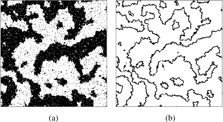
FIG. 1.: The $2D$ Ising model evolving by heat bath dynamics. (a): of a system with $250\times 250$ sites and periodic boundary conditions at temperature $T=0.9\,T_{c}$ after $500$ updates. (b): Corresponding domain walls detected by the observable $\Delta_{i}$ defined in Eq. (7). The arrows point at missing links of the contours.

The Ising model evolving by HBD or GD is defined as follows. Consider a $d$-dimensional square lattice with spins $\sigma_{i}(t)=\pm 1$. The energy at time $t$ is given by

$${H}=-\sum_{i}h_{i}(t)\sigma_{i}(t)\,,\hskip 14.22636pth_{i}(t)=\sum_{j}\sigma_{j}(t),$$ (1)

where $j$ runs over the nearest neighbors of site $i$. The local field $h_{i}(t)$ determines the transition probability $p_{i}(t)$ for the spin $\sigma_{i}$ at time $t$:

$$p_{i}(t)=\frac{e^{{h_{i}(t)}/{k_{B}T}}}{e^{{h_{i}(t)}/{k_{B}T}}+e^{{-h_{i}(t)}/{k_{B}T}}}.$$ (2)

HBD and GD differ in their update rules: In HBD the spin $\sigma_{i}$ is oriented according to the local field $h_{i}(t)$ by

$$\sigma_{i}(t+1)={\rm sgn}[p_{i}(t)-z_{i}(t)]\,,$$ (3)

where $z_{i}(t)$ are independent random numbers drawn from a uniform distribution between 0 and 1. On the other hand, in GD the spin $\sigma_{i}$ is flipped depending on its previous orientation:

$$\sigma_{i}(t+1)=\left\{\begin{array}[]{ll}\sigma_{i}(t){\rm sgn}[p_{i}(t)-z_{i}(t)]&\mbox{if $\sigma_{i}(t)=+1$}\\ \sigma_{i}(t){\rm sgn}[1-p_{i}(t)-z_{i}(t)]&\mbox{if $\sigma_{i}(t)=-1$}\end{array}\right..$$ (4)

One can easily verify that in both dynamics the probability to get $\sigma_{i}(t+1)=+1$ is the same, as expected from the equivalence between HBD and GD.

Let us now consider three replicas $A$, $B$, and $C$ and denote their spins by $\sigma^{A}_{i}(t)$, $\sigma^{B}_{i}(t)$, and $\sigma^{C}_{i}(t)$. As stated before, the initial conditions are

$$\sigma^{A}_{i}(0)={\rm sgn}[\frac{1}{2}-z^{(0)}_{i}],\qquad\sigma^{B}_{i}(0)=+1,\qquad\sigma^{C}_{i}(0)=-1\,,$$ (5)

where $z^{(0)}_{i}$ are random numbers between 0 and 1. The three replicas evolve under the same realization of noise, i.e., the same random numbers $z_{i}(t)$ are used for the updates of $\sigma^{A}_{i}(t)$, $\sigma^{B}_{i}(t)$, and $\sigma^{C}_{i}(t)$.

We now turn to the observables we want to analyze. Derrida’s definition for the fraction of persistent spins $r(t)$ can be generalized easily: A spin $\sigma^{A}_{i}(t)$ is said to be “persistent” up to time $t$ if it experienced exclusively thermal fluctuations, which means that it was synchronized either with $\sigma^{B}_{i}(t)$ or with $\sigma^{C}_{i}(t)$ for the whole time, i.e.,

$$r(t)=\frac{1}{N}\sum_{i=1}^{N}\left(\prod_{0\leq t^{\prime}\leq t}\frac{1+\sigma^{A}_{i}(t)\sigma^{B}_{i}(t)}{2}+\prod_{0\leq t^{\prime}\leq t}\frac{1+\sigma^{A}_{i}(t)\sigma^{C}_{i}(t)}{2}\right)\,,$$ (6)

where $N$ is the total number of sites. We will analyze this quantity numerically in Secs. III-IV.

In order to identify domain walls, we define an observable $\Delta_{i}(t)$ which compares replicas $A$, $B$, and $C$ at site $i$ and its nearest neighbors. We consider site $i$ as belonging to a domain wall (i.e., $\Delta_{i}(t)=1$) if (a) site $i$ or at least one of its nearest neighbors in copies $A$ and $B$ are in different states, and (b) if site $i$ or at least one of its nearest neighbors in copies $A$ and $C$ are in different states. Since HBD and GD evolve independently on two (even and odd) sublattices, we assume that these nearest neighbors belong to the same sublattice (for example, if $i=(x,y)$, the nearest neighbors on the same sublattice are $(x\pm 2,y)$ and $(x,y\pm 2)$). Formally the observable $\Delta_{i}(t)$ is defined by

$$\Delta_{i}(t)=\left(1-\prod_{j}\frac{1+\sigma^{A}_{j}(t)\sigma_{j}^{B}(t)}{2}\right)\left(1-\prod_{j}\frac{1+\sigma^{A}_{j}(t)\sigma_{j}^{C}(t)}{2}\right)\,,$$ (7)

where $j$ runs over site $i$ and its nearest neighbors on the same sublattice. It turns out that this observable allows one to identify domain walls, as illustrated for HBD in Fig. 1b.

The definition (7) appears to be quite complicated since it involves the nearest neighbors of site $i$. It would have been more natural to define a local observable $\delta_{i}(t)$, which is $1$ if $\sigma^{A}_{i}$ is different from $\sigma^{B}_{i}$ and $\sigma^{C}_{i}$ (indicating a fluctuation generated by the coarsening process) and $0$ otherwise:

$$\delta_{i}(t)=\Bigl{(}\frac{1-\sigma_{i}^{A}(t)\sigma_{i}^{B}(t)}{2}\Bigr{)}\Bigl{(}\frac{1-\sigma_{i}^{A}(t)\sigma_{i}^{C}(t)}{2}\Bigr{)}\,.$$ (8)

But, using the initial conditions specified in Eq. (5), it would turn out that $\delta_{i}(t)\equiv 0$ for all $t$ and for both HBD and GD. This is due to an overlap of the regions in $A$ which are synchronized with either $B$ or $C$. For HBD this can be proven as follows. Assume that the three replicas at time $t$ are in a state where the inequality

$$p^{C}_{i}(t)\leq p^{A}_{i}(t)\leq p^{B}_{i}(t)$$ (9)

holds for all $i$. Since the number of positive spins generated by the update rule (3) for a given random number $z_{i}(t)$ is monotonically increasing with $p_{i}(t)$, one can show that $h^{C}_{i}(t+1)\leq h^{A}_{i}(t+1)\leq h^{B}_{i}(t+1)$. Therefore the inequality (9) is also satisfied at the next time step $t+1$. Since this inequality is satisfied by the initial conditions (5), it holds by induction at any time. This implies that events with $\sigma^{A}_{i}\neq\sigma^{C}_{i}$ and $\sigma^{A}_{i}\neq\sigma^{B}_{i}$ do not occur, hence $\delta_{i}(t)\equiv 0$ for HBD. In the case of GD the proof is trivial: Since replicas $B$ and $C$ evolve precisely in opposite states ($\sigma_{i}^{B}(t)=-\sigma_{i}^{C}(t)$), the observable $\delta_{i}(t)$ vanishes automatically. Thus the local observable defined in Eq. (8) cannot be used in order to detect domain walls. This is the reason we use the more complicated definition of Eq. (7).

III Heat bath dynamics: Persistent spins and the fractal dimension of domain walls

In this section we present numerical results for the $2D$ Ising model with HBD. We simulate three replicas of a system of size $1000\times 1000$ with periodic boundary conditions. Starting with the initial conditions (5) we measure the fraction of persistent spins $r(t)$ as defined in Eq. (6) and the average Peierls length (circumference) of the domains

$$\Delta(t)=\frac{1}{N}\,\sum_{i}\Delta_{i}(t)\,.$$ (10)

The quantities $r(t)$ and $\Delta(t)$ are measured up to $5000$ time steps and averaged over $10$ independent runs. Our simulation data are shown in Figs. 2-3.

FIG. 2.: Heat bath dynamics. Measurement of the fraction of persistent spins $r(t)$ at various temperatures as a function of time (c.f. Ref. [3]). The bold line indicates the slope $-0.22$. The right hand graph shows a data collapse of the rescaled quantity $r(t)/\epsilon^{2}$ in the supercritical regime $T>T_{c}$.

FIG. 3.: Heat bath dynamics. Measurement of the total Peierls length $\Delta(t)$ at various temperatures as a function of time. The bold line indicates slope $-0.5$. The right hand graph shows the corresponding data collapse of the rescaled Peierls length $\Delta(t)/\epsilon$ in the supercritical regime.

The results for the fraction of persistent spins $r(t)$ (see left hand graph in Fig. 2) are in full agreement with Ref. [3]. For $T=0$ we observe an algebraic decay $r(t)\sim t^{-\theta}$ with $\theta=0.23\pm 0.03$. For $0\leq T<T_{c}$ $r(t)$ decreases rapidly on short time ranges while for longer times it crosses over to a $T$-independent power law decay. Precisely at the critical temperature, however, $r(t)$ seems to vanish like $r(t)\sim t^{-\theta_{c}}$ with a different exponent $\theta_{c}\simeq 1$ (the physical relevance of this exponent will be discussed in the Sec. IV). Finally, for $T>T_{c}$, $r(t)$ saturates at some finite value. This can be explained as follows. For $T>T_{c}$ the total magnetization in copies $B$ and $C$ decays exponentially. It has been shown [11] that under these conditions any difference between two replicas evolving by HBD vanishes exponentially, i.e., damage heals spontaneously. This means that the replicas $A,B,C$ converge and eventually merge into a fully synchronized evolution within finite time and consequently a finite fraction of persistent spins survives. Notice that in the limit $T\rightarrow\infty$ all replicas are already synchronized after a single time step. For finite temperatures we observe a scaling behavior (see right hand graph in Fig. 2)

$$r(t)\sim(T-T_{c})^{z}\,f(t(T-T_{c})^{z})\,,\qquad\qquad(T>T_{c})$$ (11)

where $z\simeq 2.125$ is the dynamical critical exponent of HB dynamics and $f(x)$ is a scaling function which behaves as $f(x)\sim 1/x$ for $x\rightarrow 0$ and saturates for $x\rightarrow\infty$.

The results for the total Peierls length of the domains $\Delta(t)$ illustrated in Fig. 3 indicate a power law behavior $\Delta(t)=t^{-\kappa}$ with $\kappa\simeq 0.5$ in the regime $0\leq T<T_{c}$ and an exponential decay in the disordered phase $T>T_{c}$ (to determine the behavior at $T=T_{c}$ more numerical effort would be needed, c.f. Ref. [16]) that can be explained by the synchronization of the copies within finite time. The corresponding scaling behavior reads

$$\Delta(t)\sim(T-T_{c})^{\kappa z}\,g(t(T-T_{c})^{z})\,,\qquad\qquad(T>T_{c})$$ (12)

where $g(x)$ is a scaling function as shown in the right hand graph in Fig. 3.

The exponent $\kappa\simeq 0.5$ in the subcritical regime may be interpreted as follows. The total number of domains $n(t)$ in a large but finite sized system decreases as $n(t)\sim t^{-d/2}$. Moreover, the average size of the domains $\xi$ grows with time as $\xi\sim t^{1/2}$. Hence in the $2D$ Ising model the Peierls length behaves as

$$n(t)\xi\sim\Delta(t)\sim t^{-1/2}\,.$$ (13)

This result suggests that surfaces of domains in a coarsening Ising model are regular, i.e., they do not have a fractal structure at finite temperatures $T\leq T_{c}$. This result can be explained as follows. The coarsening process is driven by the tendency of the systen to minimize its energy ${H}$, i.e., to minimize the surface area (the Peierls length $\Delta(t)$) of the domains. This makes it highly unlikely for the domain walls to form fractal structures. This mechanism works not only at zero temperature but prevails in the entire subcritical regime. To support this argument we plotted the energy ${H}$ against the Peierls length in Fig. 4. For $T<T_{c}$ the curves are monotonically decreasing with time and seem to have a well defined minimum at $\Delta=0$. This suggests that the mechanism for coarsening, apart from different time scales, is the same in the whole subcritical regime. In the disordered phase, however, the curves have a flat shape close to $\Delta=0$ and therefore the dynamics of $\Delta(t)$ is no longer driven by the minimization of energy.

FIG. 4.: Total energy ${H}(t)$ of a coarsening Ising model as a function of the Peierls length $\Delta(t)$ for various temperatures.

IV The problem of algorithmic dependence

As outlined in the Introduction, any numerical technique based on several replicas of a nonequilibrium system evolving under the same realization of noise may depend in a crucial way on the algorithmic implementation of the dynamics. We now discuss this dependence in the present problem by comparing HBD and GD.

HBD and GD are two different but equally legitimate algorithmic implementations of the same nonequilibrium process that mimics the evolution of an Ising model in contact with a thermal reservoir. To understand this, it may be helpful to rewrite the update rule for GD (4) as

$$\sigma_{i}(t+1)=\left\{\begin{array}[]{ll}{\rm sgn}[p_{i}(t)-z_{i}(t)]&\mbox{if $\sigma_{i}(t)=+1$}\\ {\rm sgn}[p_{i}(t)-\{1-z_{i}(t)\}]&\mbox{if $\sigma_{i}(t)=-1$}\end{array}\right..$$ (14)

This rule differs from HBD only inasmuch – depending on $\sigma_{i}(t)$ – the random number $z_{i}(t)$ or $1-z_{i}(t)$ is used. Since in a simulation of a single replica each random number is used only once, it makes no difference whether $z_{i}(t)$ or $1-z_{i}(t)$ enters the update rule and therefore both dynamical procedures are fully equivalent. In other words, looking at the space-time trajectory of a single Ising model, one cannot distinguish whether it was generated by HBD or GD. However, if we consider more than one replica evolving under the same noise, each random number $z_{i}(t)$ is used several times leading to different correlations $\em between$ the replicas depending on whether HBD or GD are used.

HBD and GD are two members of an infinite family of equivalent dynamical rules [13, 12]. All these rules are equally legitimate and there is no reason to prefer particular rules such as HBD or GD. Physical properties, however, should not depend on the choice of the dynamical procedure. Thus, in order to prove the algorithmic independence of a specific result, one would have to verify all these rules separately. Since this is practically impossible, we will restrict ourselves to the examples of HBD and GD. We will show that some of the previous results are affected by a change of the procedure and hence are physically irrelevant whereas others are not.

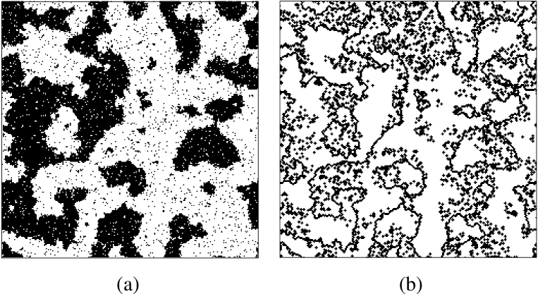
FIG. 5.: The $2D$ Ising model evolving by Glauber dynamics. (a): Snapshot of a system with $250\times 250$ sites and periodic boundary conditions at temperature $T=0.9\,T_{c}$ after $500$ time steps. (b): Corresponding domain walls detected by the observable $\Delta_{i}$. Notice that all contours are strictly closed.

We now repeat the numerical simulations described in the previous section using GD instead of HBD. A snapshot of the simulation is shown in Fig. 5. Comparing Figs. 1b and 5b we notice that the HBD algorithm yields very clean shapes for the Peierls contours while GD produces a lot of additional fluctuations. On the other hand the contours in the Glauber case are strictly closed because of symmetry reasons whereas for HBD there are missing links (two of them are marked by arrows in Fig. 1b).

We would like to note that any dynamical rule used in the present problem should synchronize the evolution of replicas $A,B$ or $A,C$ in the interior of large domains. In the terminology of DS this means that damage has to heal. As HBD is the most correlated algorithm, damage heals very rapidly and thus yields high resolution in the determination of the walls. On the other hand GD in $2D$ is known to exhibit a DS transition at $T=T_{s}\simeq 0.95\ T_{c}$ [14]. The simulations in Fig. 5b at $T=0.9\,T_{c}$ take place very close to this transition which explains why the output is rather noisy.

FIG. 6.: Glauber dynamics. Measurement of the fraction of persistent spins $r(t)$ and the total Peierls length of domain walls $\Delta(t)$ as a function of time.

The numerical results for GD and HBD are significantly different (see Fig. 6). Only at zero temperature where GD and HBD coincide does one obtain identical results. For $0<T<T_{c}$ the fraction of persistent spins $r(t)$ exhibits similar behavior in both cases: It first decays and then crosses over to an algebraic decay $r(t)\sim t^{-\theta}$ with the same $\theta\simeq 0.2$ as in the $T=0$ case. This suggests that the crossover phenomenon is an intrinsic physical property of the $2D$ Ising model rather than an algorithmic artifact. At criticality, however, GD indicates an algebraic decay $r(t)\sim t^{-2}$. This is clearly different from the decay $r(t)\sim t^{-1}$ observed in the case of HBD. Therefore one may wonder about the physical meaning of $r(t)$ at criticality. This problem may be circumvented by a systematic study of the crossover time as a function of temperature.

The results for the total Peierls length of the domains are even more contradictory. While in the HBD case we found an algebraic decay $\Delta(t)\sim t^{-1/2}$ for $0\leq T\leq T_{c}$, we observe continuously varying exponents in the case of GD. If this was true, it would imply that the Peierls length per domain grows like $\Delta(t)/n(t)\sim\xi^{\kappa}$ with some temperature-dependent exponent $\kappa>1$ indicating a “fractal” structure of the domain walls. Indeed, visual inspection of Fig. 5b makes it intuitively clear how such a “fractal” structure emerges. It is therefore tempting to discard the results for GD and to declare the smooth lines in Fig. 1b as ‘true’ domain walls. However, as explained above, we have no justification for doing so! Therefore the method described in this paper cannot be used to determine the fractal dimension of domain walls on a safe ground. Nevertheless HBD gives us a lower bound for the exponent $\kappa$. It is thus very likely, although not strictly proven, that domain walls in the coarsening Ising model at nonzero temperature do not have a fractal structure.

V Concluding remarks

By introducing three replicas of a $2D$ Ising model evolving under the same realization of noise we extend the numerical method proposed by B. Derrida [3] in a way that domain walls can be identified. Using HBD we measured the Peierls length of coarsening domains in the $2D$ Ising model. Our simulations confirm previous results and suggest that domain walls in the Ising model at $T<T_{c}$ are regular, i.e., they do not have fractal properties.

A fundamental problem appearing here and related to the use of several replicas is the algorithmic dependence. As an example we compared HBD and GD. It turns out that the persistence exponent below the critical temperature is the same in both cases which suggests that this result is in fact related to a physical property rather than algorithmic artifacts. On the other hand, the Peierls length of the domain walls grows differently for HBD and GD, although it seems that HBD gives the correct result.

In this context we would like to note that very recently a different method for the numerical estimation of the persistence exponent $\theta$ has been proposed [15] where the persistence probability is defined in terms of spin blocks. By analyzing the scaling behavior for different block sizes one can determine $\theta$ even at finite temperature. Although this method cannot be used to identify domain walls, it is very interesting since it uses only a single replica wherefore the results do not depend on whether HBD or GD is used. In agreement with Ref. [3] and the present work the authors observe that the exponent $\theta$ is the same in the entire subcritical regime. It would be interesting to use this method in order to determine $\theta$ at criticality [16].

Acknowledgments: We thank E. Domany, P. Grassberger, G. Schliecker, C. Sire and D. Stauffer for valuable discussions and comments. We also thank S. Cueille for pointing out to us the correct dynamical exponent in Eqs. (11)-(12).

REFERENCES

- [1] P. C. Hohenberg and B. I. Halperin, Rev. Mod. Phys. 49, 435 (1977); A. J. Bray, Adv. Phys. 43, 357 (1994).
- [2] A. J. Bray, J. Phys. A 23, L67 (1990); J. G. Amar and F. Family, Phys. Rev. A 41, 3258 (1990); B. Derrida and R. Zeitak, Phys. Rev. E 54, 2513 (1996).
- [3] B. Derrida, Phys. Rev. E 55, 3705 (1997).
- [4] D. Stauffer, Int. J. Mod. Phys. C 8, 361 (1997).
- [5] B. Derrida, A. J. Bray, and C. Godrèche, J. Phys. A 27, L357 (1994); D. Stauffer, J. Phys. A 27, 5029 (1994).
- [6] B. Derrida, V. Hakim, and V. Pasquier, Phys. Rev. Lett. 75, 751 (1995).
- [7] S. N. Majumdar and C. Sire, Phys. Rev. Lett. 77, 1420 (1996); S. N. Majumdar, C. Sire, A. J. Bray, and S. J. Cornell, Phys. Rev. Lett. 77, 2867 (1996); B. Derrida, Phys. Rev. Lett. 77, 2871 (1996).
- [8] S. A. Kaufmann, J. Theor. Biol. 22, 437 (1969); M. Creutz, Ann. Phys. 167, 62 (1986); B. Derrida and G. Weisbuch, Europhys. Lett. 4, 657 (1987).
- [9] P. Grassberger, J. Stat. Phys. 79, 13 (1995).
- [10] H. Hinrichsen, J. S. Weitz and E. Domany, J. Stat. Phys. 88, 617 (1997).
- [11] H. Stanley, D. Stauffer, J. Kertész and H. Herrmann, Phys. Rev. Lett. 59, 2326 (1987); A. M. Mariz, H. J. Herrmann and L. de Arcangelis, J. Stat. Phys. 59, 1043 (1990).
- [12] H. Hinrichsen and E. Domany, Phys. Rev. E 56, 94 (1997).
- [13] A. M. Mariz and H. J. Herrmann, J. Phys. A 22, L1081 (1989).
- [14] P. Grassberger, J. Phys. A 28, L67 (1995); T. Vojta, J. Phys. A 30, L7 (1997).
- [15] S. Cueille and C. Sire, unpublished (preprint cond-mat/9707287).
- [16] S. Cueille and C. Sire, in preparation.