LU TP 97-11

Revised

Statistical Properties of Unrestricted
Crew Scheduling Problems

Martin Lagerholm, Carsten Peterson and Bo Söderberg
Computational Biology and Biological Physics
University of Lund, Sölvegatan 14A, S-223 62 Lund, Sweden

Abstract:

A statistical analysis is performed for a random unrestricted local crew scheduling problem, expressed in terms of pairing arrivals with departures. The analysis is aimed at understanding the structure of similar problems with global restrictions, and estimating their difficulty. The methods developed are of a general nature and can be of use in other problems with a similar structure. For large random problems, the ground-state energy scales like $\sqrt{N}$ and the average excitation like $N$, where $N$ is the number of arrivals/departures. The average ground-state degeneracy is such that the probability of hitting an optimal pairing by chance scales like $2N2^{-N}$ for large $N$. By insisting on the local ground-state energy for a restricted problem, airports can be split into smaller parts, and the state space reduced by typically a factor $\sim 2^{N_{a}}$, with $N_{a}$ the total number of airports.

1 Introduction

Airline crew scheduling represents an important class of optimization problems where the topological structure is important. In refs. [1, 2], a novel Potts artificial neural network approach is developed for attacking semi-realistic airline crew scheduling problems of the following type: A weekly flight schedule is given in terms of a set of flights, each with a specified airport and time for departure and arrival. The object is to assign a crew to each flight, while minimizing a cost-function defined by the total required crew time (including the waiting-time at airports). The solution is subject to a set of global constraints: The crews are required to travel along closed tours, starting and ending at a certain airport, the home-base. These tours are subject to limitations as to duration and leg-count.

As shown in ref. [2], a great deal of simplification is gained by reformulating the problem as that of mapping arrivals on departures at each airport, implying an implicit representation of the crews. In fact, without the global restrictions, the problem is reduced to a set of independent local subproblems, one at each airport. Each local problem amounts to minimizing the local waiting-time, and is simply solvable in polynomial time.

In this paper, we focus on this kind of unrestricted local problems, in particular their statistical properties. These are quite interesting, and in no way trivial, in spite of the triviality of the problems. In particular, we consider the ensemble of random local problems of a fixed size $N$, as defined by the number of arrivals/departures. In addition, we analyze the properties of random solutions to such problems.

Such a statistical analysis of this type of problem does not exist in the literature, and we feel it is interesting for the following reasons: The results illuminate the structure of the corresponding restricted problems, and as a by-product, useful tools are provided for probing their difficulty, and for simplifying their solution. Some of the methods used are novel, and may be used also in other contexts, where a similar structure occurs. In addition, a lower bound to the waiting-time is provided by the solutions to the unrestricted problem. This bound is often saturated [2].

The methodology we use contains the following steps. First, the analysis of a local problem is simplified by considering its topology (defined by the relative ordering in time between arrivals and departures) separately from its geometry (defined by the lengths of the time intervals between consecutive events). The ensemble of problems is thus factorized into the direct product of the ensemble of topologies and the ensemble of geometries.

After introducing a notation for the topology, we consider problems with a fixed topology, and evaluate averages over the geometry of entities related to the waiting-time. These are simple, since the effect of the geometry on the waiting-time spectrum is a mere shift.

The apparent difficulty of a problem is probed by analyzing the distribution of waiting-times of random solutions. A nice feature is that the waiting-time spectrum for each problem is quantized in steps of the basic period of the schedule.

Subsequently, all variables of interest are averaged also over the topology. This is a more difficult task, and requires the use of a subtle recursive method.

An alternative measure of the difficulty of a problem is the ground-state degeneracy, i.e. the number of solutions with minimal waiting-time, as compared to the total number of solutions, given by $N!$. This is independent of geometry. Due to the character of the dependence on topology, non-standard methods are required to compute the average over topology.

This paper is organized as follows: In Section 2, the problem ensemble is defined. In Section 3, a formalism is introduced for characterizing the topology. The degeneracy structure as a function of topology is analyzed, and various energy moments for fixed topology are computed, by averaging over geometry and/or pairing. In Section 4, a statistical analysis of the detailed degeneracy structure is considered. In particular, the average ground-state degeneracy is computed. Section 5 contains our conclusions.

2 Unrestricted Crew Scheduling

2.1 The Local Problem

A local problem of size $N$ is defined by specifying the times for $N$ arrivals (arr’s) and $N$ departures (dep’s), denoted respectively by $t^{a}_{i}$ and $t^{d}_{i},\;i=1\ldots N$. The object is simply to find a one-to-one mapping (a pairing) between the arr’s and dep’s, such that the energy (or objective function) $E$, given by the total waiting-time, is minimal. In general this can be done in more than one way, implying a degeneracy of the ground-state.

The pairing of an arr $A$ with a dep $D$ implies that the crew assigned to $A$ should next be assigned to $D$. The periodicity of the schedule implies that any arr may be mapped on any dep: if the dep is earlier, it is taken as the same dep in the next period.

In what follows, we will use the period as the unit of time (and thus energy). Then the times for the arr’s and dep’s can be restricted to the unit interval. If an arr $i$ is mapped on a dep $j$, their contribution to the total waiting-time is given by

$$t^{w}_{ij}=\left(t^{d}_{j}-t^{a}_{i}\right)\mbox{ mod }1\;\in[0,1].$$ (1)

Thus, whatever the mapping, the energy $E$ is restricted to the interval $[0,N]$, and between different pairings it can only change by an integer amount. Pairings yielding the lowest possible energy $E_{0}$ are said to belong to the ground-state, while a pairing with $E=E_{0}+k,\;k>0$ is said to belong to $k$:th excited state.

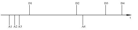
Figure 1: An example of a local flight schedule.

In figure 1, an example of a flight schedule is depicted.

2.2 The Random Local Problem

A random local problem is defined by independently choosing the times for $N$ arr’s and $N$ dep’s randomly on the unit period. It is useful to divide the characterization of a given problem in two parts: its topology and its geometry. The topology is defined by the relative ordering in the combined (cyclic) sequence of arr’s and dep’s. The probability is the same for every distinct topology. The geometry is defined by the sizes of the $2N$ inter-spaces $x_{i},i=1,\ldots,2N$, into which the period is divided.

For a given problem, the solution space is defined by the set of pairings, i.e. the $N!$ possible mappings between arr’s and dep’s.

We will be interested mainly in the statistical properties of the following entities: the ground-state energy (minimal waiting-time) $E_{0}$, the energy $E$ of a random pairing, and the (integer) difference $D=E-E_{0}$ defining the excitation energy. We will also be interested in the degeneracies of the ground-state and the excited states. To that end, we will consider three kinds of averages: over respectively the topology, the geometry, and the pairing.

The degeneracies of the ground-state and the excited states depend only on the topology, i.e. the combined ordering of arr’s and dep’s.

For a fixed topology, the excitation energy $D$ is independent of the geometry, and depends entirely on the pairing. Conversely, the ground-state energy $E_{0}$ obviously is independent of the pairing, and depends only on the geometry. Thus, for a fixed topology, $D$ and $E_{O}$ are completely uncorrelated, in the combined ensemble of random geometries and random pairings.

3 Analysis for Fixed Topology

3.1 Characterization of the Topology

A simple way to achieve a ground-state pairing (i.e. solve the problem) for a given topology is as follows:

1. An arr immediately followed by a dep is paired with that dep, and both are removed from the sequence. Note that the dep could be in the next period.

2. The process is continued until all arr’s and dep’s are used.

As an example, consider the sequence $[A_{1}A_{2}A_{3}D_{1}D_{2}A_{4}D_{3}D_{4}]$, corresponding to the topology of the schedule in figure 1.

• Pairing $A_{3}$ with $D_{1}$ leaves $[A_{1}A_{2}D_{2}A_{4}D_{3}D_{4}]$.

• Pairing $A_{2}$ with $D_{2}$ leaves $[A_{1}A_{4}D_{3}D_{4}]$.

• Pairing $A_{4}$ with $D_{3}$ leaves $[A_{1}D_{4}]$.

• Pairing $A_{1}$ with $D_{4}$ finishes the process.

A graphical representation of the topology is now defined as follows.

• If necessary, rotate the sequence such that no pairing crosses the interval border.

• Represent the arr’s and dep’s by equally spaced points on the interval.

• For each pairing in turn, draw a line from the arr to the dep on the lowest level (one). All previously drawn lines that overlap with the new line are lifted one level.

Thus a set of lines at different levels are obtained, each line starting at an arr and ending on a dep. For the example above, the result is shown in fig. 2. Each line represents a crew waiting for a dep.

Figure 2: Graphical representation of the topology $[AAADDADD]$

It turns out that for the properties of the total energy spectrum, full knowledge of the topology is not necessary; it suffices to know how many lines there are at the different levels. Thus let $P_{k}$ be the number of lines at level $k$ ($k=1,2,3,\ldots$). For the example above, the $P$ sequence is $[1,2,1]$, i.e. $P_{1}=1,P_{2}=2,P_{3}=1$, while $P_{k}=0$ for $k>3$.

3.2 Degeneracy Structure

The ground-state degeneracy is now given by the product of the line-levels, i.e.

$$g_{0}=\prod_{k\geq 1}k^{P_{k}}.$$ (2)

This is because each dep must terminate a line, and the number of available crews is equal to the number of lines alive at that point, which is given by the line’s level. For the example we get $3\times 2\times 2\times 1=12$, corresponding to half of the 24 possible pairings.

Naively, the degeneracy of the $m$th excited state can be obtained by adding $m$ dummy lines, covering the entire interval; they represent extra crews. Then each dep has $m$ additional crews to choose between, and we get for the naive degeneracy

$$a_{m}=\prod_{k\geq 1}(k+m)^{P_{k}},$$ (3)

where we have assumed indistinguishable dummy lines; otherwise we would have an extra factor $m!$. This defines an infinite sequence.

However, some of the possible pairings will contain permanently grounded crews (closed lines), or lines extending over more than one period. The contribution to the naive multiplicity from solutions with $n$ grounded crews and/or excessive periods depends on the proper degeneracy $n$ steps down. Denoting the proper degeneracies by $g_{m}$, the relation is

$$a_{m}=\sum_{n=0}^{m}g_{m-n}\left(\begin{array}[]{c}N+n\\ n\end{array}\right),$$ (4)

where the last factor is a binomial coefficient. This represents a kind of renormalization, and can be inverted to yield the proper degeneracies

$$g_{m}=\sum_{n=0}^{m}a_{m-n}(-)^{n}\left(\begin{array}[]{c}N+1\\ n\end{array}\right).$$ (5)

This must define a finite sequence, since $g_{m}\geq 0$ and the total number of pairings, $\sum_{m}g_{m}=N!$, is finite.

From eq. (3), it is obvious that the naive degeneracy $a_{m}$ is an $N$th degree polynomial in $m$; hence it can be written as

$$a_{m}=\sum_{k=0}^{N}c_{k}\left(\begin{array}[]{c}m+k\\ k\end{array}\right),$$ (6)

with some coefficients $c_{k}$. Define the generating functions

$$A(x)=\sum_{m}a_{m}x^{m}\;,\;\;G(x)=\sum_{m}g_{m}x^{m}.$$ (7)

Due to eq. (5), these are related by $G(x)=(1-x)^{N+1}A(x)$. Then, in terms of $c_{k}$, we have

$$A(x) = \sum_{k=0}^{N}c_{k}(1-x)^{-k-1},$$ (8)

$$G(x) = \sum_{k=0}^{N}c_{k}(1-x)^{N-k}.$$ (9)

From this, we see that the $g$ sequence is indeed finite: $g(m)=0$ for all $m>N$. The individual degeneracies $g_{m}$ can be obtained from $G$ and its derivatives at $x=0$,

$$g_{0} = G(0)\;=\;\sum_{k}c_{k},$$ (10)

$$g_{1} = G^{\prime}(0)\;=\;-\sum_{k=0}^{N}(N-k)c_{k},$$

etc.

3.3 The Excitation Energy for a Random Pairing

Conversely, the moments over $g_{m}$ are readily obtained from $G$ and its derivatives at $x=1$,

$$\sum_{m}g_{m} = G(1)\;=\;c_{N},$$ (11)

$$\sum_{m}mg_{m} = G^{\prime}(1)\;=\;-c_{N-1},$$

$$\sum_{m}m(m-1)g_{m} = G^{\prime\prime}(1)\;=\;2c_{N-2},$$

etc. In order to relate $c_{k}$ to $P_{k}$, we can express the coefficients of the polynomial $a_{m}$ in two different ways. From eq. (3) we get for the leading coefficients

$$a_{m}=m^{N}+m^{N-1}\sum_{k}kP_{k}+\frac{m^{N-2}}{2}\left\{\left(\sum_{k}kP_{k}\right)^{2}-\sum_{k}k^{2}P_{k}\right\}+\ldots,$$ (12)

while eq. (6) gives, upon expanding the binomial coefficients,

$$a_{m} = \frac{m^{N}}{N!}c_{N}\;+\;\frac{m^{N-1}}{N!}\left\{\frac{1}{2}N(N+1)c_{N}+Nc_{N-1}\right\}$$

$$+ \frac{m^{N-2}}{N!}\left\{\frac{1}{24}N(N-1)(N+1)(3N+2)c_{N}+\frac{1}{2}N^{2}(N-1)c_{N-1}+N(N-1)c_{N-2}\right\}+\ldots$$

From this we obtain the relations

$$c_{N} = N!,$$ (14)

$$c_{N-1} = N!\left\{\frac{1}{N}\sum_{k}kP_{k}-\frac{N+1}{2}\right\},$$

$$c_{N-2} = N!\left\{\frac{1}{2N(N-1)}\left(\sum_{k}kP_{k}\right)^{2}-\frac{1}{2N(N-1)}\sum_{k}k^{2}P_{k}-\frac{1}{2}\sum_{k}kP_{k}+\frac{(N+1)(3N-2)}{24}\right\},$$

etc. This gives (as it should) $\sum_{m}g_{m}=N!$, the number of possible pairings. In a given topology, the fraction of pairings having an energy $D=m$ steps above $E_{0}$ is given by $g_{m}/N!$. Thus, the first few moments of the excitation energy $D$ for a random pairing are:

$$<D>_{p} = \frac{1}{N!}\sum_{m}mg_{m}\;=\;\frac{N+1}{2}-\frac{1}{N}\sum_{k}kP_{k},$$

$$<D^{2}>_{p} = \frac{1}{N!}\sum_{m}m^{2}g_{m}$$

$$= \frac{1}{N(N-1)}\left(\sum_{k}kP_{k}\right)^{2}-\frac{1}{N(N-1)}\sum_{k}k^{2}P_{k}-\frac{N+1}{N}\sum_{k}kP_{k}+\frac{(N+1)(3N+4)}{12},$$

where $<>_{p}$ denotes the average over pairings for a fixed topology.

3.4 The Ground-State Energy in a Random Geometry

For a given topology, the ground-state energy depends on the geometry, and is given by

$$E_{0}=\sum_{i=1}^{2N}k_{i}x_{i},$$ (16)

where $x_{i}$ is the length of the $i$th sub-interval, and $k_{i}$ the number of lines in that interval.

To perform averages over a random geometry, we need to analyze the distribution of the intervals $x_{i}$. Independently of the topology, they obey the distribution

$$dP=(2N-1)!\;\delta\left(\sum_{i}x_{i}-1\right)\prod_{i=1}^{2N}\left(\Theta(x_{i})dx_{i}\right).$$ (17)

For a single $x_{i}$, this implies the distribution

$$f(x_{i})=(2N-1)\left(1-x_{i}\right)^{2N-2}\;,\;0\leq x_{i}\leq 1.$$ (18)

Using the identity $\sum_{i}x_{i}=1$, and the permutation symmetry between different $x_{i}$, we have

$$<x_{i}> = \frac{1}{2N},$$ (19)

$$<x_{i}x_{j}> = \frac{1+\delta_{ij}}{2N(2N+1)}.$$ (20)

In what follows, we will also need the number of intervals with $k$ lines, to be denoted by $Q_{k}$; in terms of $P_{k}$ (defining $P_{0}=0$) it is simply

$$Q_{k}=P_{k}+P_{k+1},\;k\geq 0,$$ (21)

since adding a line on level $k$ implies adding two intervals, with respectively $k$ and $k-1$ lines. Obviously, we have $\sum_{k}Q_{k}=2N$.

Now we are ready to compute the first few moments of $E_{0}$, yielding

$$<E_{0}>_{g} = \sum_{i=1}^{2N}k_{i}<x_{i}>_{g}=\frac{1}{2N}\sum_{i}k_{i}=\frac{1}{2N}\sum_{k}kQ_{k}=\frac{1}{N}\sum_{k}kP_{k}-\frac{1}{2},$$

$$<E_{0}^{2}>_{g} = \sum_{ij}k_{i}k_{j}<x_{i}x_{j}>=\frac{1}{2N(2N+1)}\sum_{ij}k_{i}k_{j}(1+\delta_{ij})$$

$$= \frac{1}{2N(2N+1)}\left(\sum_{kl}klQ_{k}Q_{l}+\sum_{k}k^{2}Q_{k}\right)$$

$$= \frac{1}{2N(2N+1)}\left(4\left(\sum_{k}kP_{k}\right)^{2}+2\sum_{k}k^{2}P_{k}-2(2N+1)\sum_{k}kP_{k}+N(N+1)\right),$$

where $<>_{g}$ denotes average over the geometry for fixed topology.

3.5 The Total Energy

The total energy $E$ is given by the ground-state and excitation energies, $E=E_{0}+D$. Averaging over both geometry and pairing, we obtain the surprisingly simple result

$$<E>_{gp}\,=\,<E_{0}>_{g}+<D>_{p}\,=\,\frac{N}{2},$$ (23)

independently of topology.

Since we already have the second moments of $E_{0}$ and $D$, we only need $<E_{0}D>$ to compute the second moment of $E$. Using the fact that $E_{0}$ and $D$ are statistically independent for a fixed topology, we get

$$<E_{0}D>_{gp}\,=\,<E_{0}>_{g}<D>_{p}\,=\,-\frac{1}{N^{2}}\left(\sum_{k}kP_{k}\right)^{2}+\frac{N+2}{2N}\sum_{k}kP_{k}-\frac{N+1}{4}.$$ (24)

This implies

$$<E^{2}>_{gp}=\frac{2(N^{2}+N+1)}{N^{2}(N-1)(2N+1)}\left(\sum_{k}kP_{k}\right)^{2}-\frac{3(N+1)}{N(N-1)(2N+1)}\sum_{k}k^{2}P_{k}+\frac{(N+1)(6N^{2}-N+4)}{12(2N+1)}.$$ (25)

4 Topology Statistics

4.1 The Topology Ensemble

We now want to perform averages also over the topology, for the moments of the ground-state energy $E_{0}$, the excitation energy $D$, and the total energy $E$.

$N$	Pattern	Prob.	$\{P_{k}\}$	$\{Q_{k}\}$	$\{a_{i}\}$	$\{g_{i}\}$	$\langle E_{0}\rangle$	$\langle D\rangle$
1	AD	1	[1]	[1,1]	1,2,3,…	(1)	1/2	0
2	AADD	2/3	[1,1]	[1,2,1]	2,6,12,…	(2)	2/2	0
2	ADAD	1/3	[2]	[2,2]	1,4,9,…	(1,1)	1/2	1/2
3	AAADDD	3/10	[1,1,1]	[1,2,2,1]	6,24,60,…	(6)	9/6	0
3	AADADD	3/10	[1,2]	[1,3,2]	4,18,48,…	(4,2)	7/6	1/3
3	AADDAD	3/10	[2,1]	[2,3,1]	2,12,36,…	(2,4)	5/6	2/3
3	ADADAD	1/10	[3]	[3,3]	1,8,27,…	(1,4,1)	3/6	3/3
4	AAAADDDD	4/35	[1,1,1,1]	[1,2,2,2,1]	24,120,360,…	(24)	8/4	0
4	AAADADDD	4/35	[1,1,2]	[1,2,3,2]	18,96,300,…	(18,6)	7/4	1/4
4 4	AAADDADD AADAADDD	$\left.\parbox{19.91692pt}{4/35 4/35}\right\}$	[1,2,1]	[1,3,3,1]	12,72,240,…	(12,12)	6/4	2/4
4	AAADDDAD	4/35	[2,1,1]	[2,3,2,1]	6,48,180,…	(6,18)	5/4	3/4
4	AADADADD	4/35	[1,3]	[1,4,3]	8,54,192,…	(8,14,2)	5/4	3/4
4 4	AADDAADD AADADDAD	$\left.\parbox{19.91692pt}{2/35 4/35}\right\}$	[2,2]	[2,4,2]	4,36,144,…	(4,16,4)	4/4	4/4
4	AADDADAD	4/35	[3,1]	[3,4.1]	2,24,108,…	(2,14,8)	3/4	5/4
4	ADADADAD	1/35	[4]	[4,4]	1,16,81,256,…	(1,11,11,1)	2/4	6/4

Table 1: Inequivalent topologies for $N\leq 4$. For each topology, the third column gives the probability of occurrence, while the next two give its $P_{k}$ and $Q_{k}$ sequence, respectively. In the following two columns the $a_{i}$ and $g_{i}$ sequences are given, whereas the last two columns give the average ground-state energy and excitation, respectively. Note that different topologies might have identical characteristics in terms of $P_{k}$, etc.

In table 1 a complete list of topologies for $N$ up to four is given, along with various characteristics. Note the similarity in symmetry-properties between the $P$, $Q$ and $g$ sequences.

To compute $<P_{k}>$, we must analyze the number of ways $m[P]$ to obtain a given $P$ sequence.

• The lowest level lines define $P_{1}$ non-overlapping subgroups; these are cyclically indistinguishable, so the naive multiplicity must be divided by $P_{1}$.

• For the $P_{k}$ indistinguishable lines on a higher level $k$, there are $P_{k-1}$ possible lines on the previous level to put them above. This can be done in $\left(\begin{array}[]{c}P_{k}+P_{k-1}-1\\ P_{k}\end{array}\right)$ ways.

• In addition, there are $2N$ cyclic rotations of the $AD$ sequence that yield the same topology.

• The $P$ sequence must sum up to $N$, and $P_{1}$ must not vanish.

This gives for the multiplicity $m[P]$

$$m[P]=\frac{2N}{P_{1}}\delta_{N-\sum P_{k}}\prod_{k=1}^{\infty}\left(\begin{array}[]{c}P_{k}+P_{k+1}-1\\ P_{k+1}\end{array}\right).$$ (26)

The total number of possible topologies for a fixed $N$ is simply the number of possible $AD$ sequences, i.e. the number of distinct orderings of a sequence of $N$ $A$’s and $N$ $D$’s. This is given by $\left(\begin{array}[]{c}2N\\ N\end{array}\right)$. This should match the total multiplicity $M_{N}\equiv\sum_{[P]}m([P])$, which can be recursively obtained from $m[P]$ by expanding the Kronecker delta in terms of a complex integral along a small contour $C$ around the origin:

$$\delta_{N-\sum P_{k}}=\oint_{C}\frac{dz}{2\pi iz^{N+1}}\prod z^{P_{k}}.$$ (27)

By iteratively using the identity

$$z^{a}\sum_{b=0}^{\infty}\left(\begin{array}[]{c}a+b-1\\ a-1\end{array}\right)w^{b}=z^{a}\sum_{b=0}^{\infty}\left(\begin{array}[]{c}-a\\ b\end{array}\right)(-w)^{b}=\left(\frac{z}{1-w}\right)^{a}.$$ (28)

when summing $m[P]\prod z^{P_{k}}$ over the $P_{k}$ in order of decreasing $k$, we obtain convergence of the power factor to $\omega^{P_{k}}$, with $\omega$ given by

$$\omega=\frac{z}{1-\omega}\;\Rightarrow\;\omega=\frac{1}{2}\left(1-\sqrt{1-4z}\right).$$ (29)

Thus, the total multiplicity is given by

$$M_{N}=2N\oint_{C}\frac{dz\;z^{-N}}{2\pi iz}\sum_{P_{1}}\frac{\omega(z)^{P_{1}}}{P_{1}}=2N\oint_{C}\frac{dz\;z^{-N}}{2\pi iz}\left(-log(1-\omega(z))\right)=\left(\begin{array}[]{c}2N\\ N\end{array}\right),$$ (30)

obtained by extracting the $z^{N}$ coefficient of $-\log(1-\omega(z))$ as $\frac{1}{2N}\left(\begin{array}[]{c}2N\\ N\end{array}\right)$, by doing the integral in terms of $w$ using $z=w(1-w)$.

4.2 Distribution of $P_{1}$

The number of non-overlapping groups of lines is given by the number of lines at level 1, i.e. $P_{1}$. In fact, $w(z)$ can be seen as a generating function,

$$w(z)=\sum_{n=1}^{\infty}m^{(1)}_{n}z^{n}=-\frac{1}{2}\sum_{n=1}^{\infty}(4z)^{n}\left(\begin{array}[]{c}n-\frac{3}{2}\\ n\end{array}\right)=\frac{1}{2}\sum_{n=1}^{\infty}(2z)^{n}\frac{(2n-3)!!}{n!},$$ (31)

for the number of ways ($m^{(1)}_{n}$) to arrange $n$ lines in such a group. The distribution of $P_{1}$ is easy to compute by slightly modifying eq. (30): skipping the summation over $P_{1}$ and dividing by $M_{N}$ yields

$$\mbox{Prob}(P_{1})=\frac{2N}{\left(\begin{array}[]{c}2N\\ N\end{array}\right)}\oint_{C}\frac{dz\;z^{-N}}{2\pi iz}\frac{\omega(z)^{P_{1}}}{P_{1}}=\frac{N!(2N-1-P_{1})!}{(2N-1)!(N-P_{1})!}$$ (32)

for $P_{1}>0$. For large $P_{1}\ll N$, this is close to $2^{-P_{1}}$.

The grouping of lines corresponds to a grouping of the flights, with a matching number of arr’s and dep’s in each group. In a ground-state pairing, flights in different groups are never paired, and within a group, the arr has to precede its paired dep. This fact can be used to simplify also restricted problems.

4.3 Moments of $P_{k}$

Similarly, $<P_{k}>$ can be obtained from realizing that inserting a factor $P_{k}$ in the sum over $P_{k}$ gives a factor $P_{k-1}\omega/(1-\omega)$. This yields in the end an extra factor $P_{1}(\omega/(1-\omega))^{k-1}$ in the $P_{1}$ sum:

$$M_{N}<P_{k}> = 2N\oint_{C}\frac{dz}{2\pi iz^{N+1}}\left(\frac{\omega}{1-\omega}\right)^{k-1}\sum_{P_{1}>1}\omega^{P_{1}}$$ (33)

$$= 2N\oint_{C}\frac{dz}{2\pi iz^{N+1}}\left(\frac{\omega}{1-\omega}\right)^{k}$$ (34)

$$= 2N\oint_{C}\frac{d\omega(1-2\omega)}{2\pi i\omega^{N-k+1}(1-\omega)^{N+k+1}},$$ (35)

where the last expression is a reformulation in terms of a loop integral around $\omega=0$. In a similar way $<P_{k}P_{l}>$ etc. can be computed. We obtain

$$<P_{k}> = \frac{2N}{M_{N}}\left\{\left(\begin{array}[]{c}2N-1\\ N-k\end{array}\right)-\left(\begin{array}[]{c}2N-1\\ N-k-1\end{array}\right)\right\}=\frac{2k}{M_{N}}\left(\begin{array}[]{c}2N\\ N-k\end{array}\right),$$ (42)

$$<P_{k}P_{m}> = \frac{2N}{M_{N}}\left\{\left(\begin{array}[]{c}2N\\ N-m\end{array}\right)-\left(\begin{array}[]{c}2N\\ N-k-m\end{array}\right)\right\},\;k\leq m.$$ (47)

From these expressions, we can derive the following particular averages, needed to compute the various energy moments over the topology:

$$\left\langle\sum_{k}kP_{k}\right\rangle = \frac{N}{2}4^{N}\left(\begin{array}[]{c}2N\\ N\end{array}\right)^{-1}\approx\frac{N}{2}\sqrt{\pi N}\left(1+\frac{1}{8N}+\ldots\right),$$ (50)

$$\left\langle\sum_{k}k^{2}P_{k}\right\rangle = N^{2},$$ (51)

$$\left\langle\left(\sum_{k}kP_{k}\right)^{2}\right\rangle = \frac{N^{2}(5N+1)}{6},$$

where the approximate form in the top equation is valid for large $N$.

4.4 Full Energy Averages

We are now ready to compute the final averages also over the topology. Inserting the results of eqs. (51) into eqs. (3.4), we obtain for the moments of the ground-state energy $E_{0}$ of a random problem:

$$<E_{0}> = \frac{1}{2}4^{N}\left(\begin{array}[]{c}2N\\ N\end{array}\right)^{-1}-\frac{1}{2}\;\approx\;\frac{1}{2}\sqrt{\pi N}-\frac{1}{2},$$ (54)

$$<E_{0}^{2}> = \frac{5N}{6}-\frac{1}{2}4^{N}\left(\begin{array}[]{c}2N\\ N\end{array}\right)^{-1}+\frac{1}{2}\;\approx\;\frac{5N}{6},$$ (57)

$$<E_{0}^{2}>_{c} \approx \frac{(10-3\pi)N}{12},$$

where $\langle ab\rangle_{c}=\langle ab\rangle-\langle a\rangle\langle b\rangle$ is the connected moment; the approximate forms are valid for large $N$.

Similarly, from eqs. (3.3) we get for the moments of the excitation energy $D$, for a random pairing in a random topology,

$$<D> = \frac{N+1}{2}-\frac{1}{2}4^{N}\left(\begin{array}[]{c}2N\\ N\end{array}\right)^{-1}\;\approx\;\frac{N}{2}-\frac{1}{2}\sqrt{\pi N}+\frac{1}{2},$$ (60)

$$<D^{2}> = \frac{N^{2}}{4}+\frac{17N}{12}+\frac{1}{3}-\frac{N+1}{2}4^{N}\left(\begin{array}[]{c}2N\\ N\end{array}\right)^{-1}$$

$$\approx \frac{N^{2}}{4}-\frac{N}{2}\sqrt{\pi N}+\frac{17N}{12},$$

$$<D^{2}>_{c} \approx \frac{(11-3\pi)N}{12}.$$ (64)

Averaging the combined moment, eq. (24), over topology yields

$$<E_{0}D> = \frac{N+2}{4}4^{N}\left(\begin{array}[]{c}2N\\ N\end{array}\right)^{-1}-\frac{13N+5}{12}\;\approx\;\frac{N}{4}\sqrt{\pi N}-\frac{13N}{12},$$ (67)

$$<E_{0}D>_{c} = -\frac{5N+1}{6}+\frac{1}{4}16^{N}\left(\begin{array}[]{c}2N\\ N\end{array}\right)^{-2}\;\approx\;-\frac{(10-3\pi)N}{12}.$$ (70)

Combining this with the moments of $E_{0}$ and $D$, we get for the moments of the total energy, $E=E0+D$, the following simple results

$$<E> = \frac{N}{2},$$ (71)

$$<E^{2}> = \frac{N^{2}}{4}+\frac{N}{12},$$ (72)

$$<E^{2}>_{c} = \frac{N}{12},$$ (73)

which can be understood by noting that a random pairing in a random topology corresponds to a set of $N$ lines with random endpoints. Then each line has a uniform length distribution between 0 and 1, and $E$ is their total length.

Computing the corresponding standard deviations, we have for a typical random problem (and a random pairing, for $D$ and $E$) at large $N$,

$$E_{0} \sim \frac{1}{2}\sqrt{\pi N}\;\pm\;\frac{1}{2}\sqrt{\left(\frac{10}{3}-\pi\right)N},$$ (74)

$$D \sim \frac{N}{2}-\frac{1}{2}\sqrt{\pi N}\;\pm\;\frac{1}{2}\sqrt{\left(\frac{11}{3}-\pi\right)N},$$ (75)

$$E \sim \frac{N}{2}\;\pm\;\frac{1}{2}\sqrt{\frac{N}{3}},$$ (76)

and we see that $E$ scales as $\sqrt{N}$, while $E$ and $D$ scale as $N$, while the standard deviation scales as $\sqrt{N}$ in each case.

Of interest are also the correlations at large $N$, given to order $N$ by

$$<E_{0}D>_{c} \sim -\frac{N}{12}(10-3\pi),$$

$$<E_{0}E>_{c} \sim 0,$$ (77)

$$<DE>_{c} \sim \frac{N}{12},$$

indicating that $E$ and $E_{0}$ become uncorrelated for a random pairing of a large random problem.

4.5 Statistics for Individual Degeneracies

An interesting but more difficult thing to compute is the average fraction $\gamma_{n}=<g_{n}>/N!$ of pairings having a given excitation energy $D=n$, in particular the ground-state fraction $\gamma_{0}$, which gives the average probability of hitting a ground-state by chance. Since $g_{n}$ is simply related to $a_{n}$, we will start by considering

$$\alpha_{n}=\frac{\left(\begin{array}[]{c}2N\\ N\end{array}\right)}{2N}<a_{n}>,$$ (78)

in terms of which $\gamma_{n}$ can be expressed as

$$\gamma_{n}=\frac{N!}{(2N-1)!}\sum_{m}(-)^{m}\left(\begin{array}[]{c}N+1\\ m\end{array}\right)\alpha_{n-m}.$$ (79)

We then have

$$\alpha_{n}=\frac{1}{2N}\sum_{[P]}m[P]\prod_{k}(n+k)^{P_{k}}=\sum_{[P]}\frac{1}{P_{1}}\delta_{N-\sum P_{k}}\prod_{k\geq 1}(n+k)^{P_{k}}\left(\begin{array}[]{c}P_{k}+P_{k+1}-1\\ P_{k+1}\end{array}\right).$$ (80)

A generating function for the $N$-dependence of $\alpha_{n}$ is then

$$A_{n}(z)\equiv\sum_{N}z^{N}\alpha_{n}(N)=\sum_{[P]}\frac{1}{P_{1}}\prod_{k\geq 1}[z(n+k)]^{P_{k}}\left(\begin{array}[]{c}P_{k}+P_{k+1}-1\\ P_{k+1}\end{array}\right).$$ (81)

Again, starting the $P_{k}$ summation at a large $k_{0}$ and proceeding in order of decreasing $k$, gives convergence of the full sum in the limit $k_{0}\to\infty$. Denoting by $\omega_{k+n-1}^{P_{k}}$ the result of summing above a certain $k$, we have by eq. (28),

$$\omega_{k-1}=\frac{kz}{1-w_{k}},$$ (82)

and the final result is

$$A_{n}(z)=\sum_{P_{1}}\frac{1}{P_{1}}\omega_{n}^{P_{1}}=-\log\left(1-\omega_{n}(z)\right).$$ (83)

The recursion relation (82) can now be linearized by assuming $\omega_{k}=p_{k}/q_{k}$, which can be solved e.g. by

$$q_{k-1} = q_{k}-p_{k},$$ (84)

$$p_{k-1} = kzq_{k},$$ (85)

which, upon eliminating $p_{k}$ gives

$$kzq_{k}-q_{k-1}+q_{k-2}=0.$$ (86)

By partial integration, it is simple to prove that the following sequence of integrals solves the recursion relation (86) for $q_{k}$,

$$q_{k}=\mbox{Im}\int_{0}^{\infty}\frac{(-iy)^{k}}{k!}\exp\left(-z\frac{y^{2}}{2}+iy\right)dy\;,\;k\geq 0,\;z>0,$$ (87)

which can be extended to negative $k$ by recursion. The $q_{k}$ can be expanded in $z$ as

$$q_{k}=\left\{\begin{array}[]{l}{}\sum_{m=0}^{\infty}\left(\begin{array}[]{c}2m+k\\ 2m\end{array}\right)(2m-1)!!z^{m}\;,\;k\geq 0,\\ \sum_{m=0}^{[-(k+1)/2]}\left(\begin{array}[]{c}-k-1\\ 2m\end{array}\right)(2m-1)!!z^{m}\;,\;k<0,\end{array}\right.$$ (88)

where $[\,]$ denotes integer part. Note that for non-negative $k$ the series is an asymptotic one, while for negative $k$ it is finite. In particular, we have $q_{-1}=1$. An independent solution to (86) is given by

$$\hat{q}_{k}(z)=\frac{z^{-k}}{k!}q_{-k-1}(-z),$$ (89)

but this solution is irrelevant, having the wrong large-$k$ behaviour.

In terms of $q_{k}$ we now have

$$1-\omega_{k} = q_{k-1}/q_{k},$$ (90)

$$A_{n} = \log\left(q_{n}\right)-\log\left(q_{n-1}\right),$$ (91)

which should then be expanded in powers of $z$ to yield $\alpha_{n}(N)$ as the coefficient of $z^{N}$. In particular, we have $A_{0}=\log(q_{0})$, where $q_{0}=1+z+3z^{2}+15z^{3}+\ldots$.

In table 2, results are displayed for the average degeneracy of the two lowest states, based on an expansion of $A_{0}$ and $A_{1}$ in powers of $z$.

$N$	$K_{N}=\frac{1}{2}\left(\begin{array}[]{c}2N\\ N\end{array}\right)$	$K_{N}<g_{0}>$	$K_{N}<g_{1}>$	$<g_{0}>$	$<g_{1}>$	$\gamma_{0}$	$\gamma_{1}$
1	1	1	0	1.00000	0.00000	1.000000	0.000000
2	3	5	1	1.66667	0.33333	0.833333	0.166667
3	10	37	22	3.70000	2.20000	0.616667	0.366667
4	35	353	411	10.0857	11.7429	0.420238	0.489286
5	126	4081	7676	32.3889	60.9206	0.269907	0.507672
6	462	55205	149741	119.491	324.115	0.165960	0.450159
7	1716	854197	3.09875$\times 10^{6}$	497.784	1805.80	0.098767	0.358294
8	6435	1.4876$\times 10^{7}$	6.84187$\times 10^{7}$	2311.74	10632.3	0.057335	0.263697
9	24310	2.88019$\times 10^{8}$	1.61447$\times 10^{9}$	11847.7	66411.7	0.032649	0.183013
10	92378	6.13891$\times 10^{9}$	4.07031$\times 10^{10}$	66454.3	440614.	0.018313	0.121421
11	352716	1.42882$\times 10^{11}$	1.09496$\times 10^{12}$	405092.	3.10436$\times 10^{6}$	0.010148	0.077771
12	1.35208$\times 10^{6}$	3.60668$\times 10^{12}$	3.13708$\times 10^{13}$	2.66751$\times 10^{6}$	2.32019$\times 10^{7}$	0.005569	0.048438
13	5.20030$\times 10^{6}$	9.81584$\times 10^{13}$	9.55147$\times 10^{14}$	1.88755$\times 10^{7}$	1.83672$\times 10^{8}$	0.003031	0.029496
14	2.00583$\times 10^{7}$	2.86562$\times 10^{15}$	3.08337$\times 10^{16}$	1.42865$\times 10^{8}$	1.5372$\times 10^{9}$	0.001639	0.017633

Table 2: Results for the average degeneracy of the lowest energy-states for various system sizes $N$. The second column gives an integer normalization factor $K_{N}$. Dividing the integers in the next two columns by $K_{N}$ yields the average number of ground-states $<g_{0}>$ and first excited states $<g_{1}>$, respectively. Dividing these by $N!$ yields $\gamma_{0}$ and $\gamma_{1}$.

It is easy to check for small $N$, using table 1, that $g_{m}/\sum g_{k}$ for $m=0,1$, averaged over topologies with the proper probabilities, indeed agrees with $\gamma_{m}$ of table 2, obtained from the expansion of $A_{k}$.

The result for $\gamma_{0}$ strongly indicates an asymptotic behaviour of $\gamma_{0}\sim 2N2^{-N}$. This corresponds to an exponential decrease with $N$ of the average probability for a random pairing to hit a ground-state. However, the average number of ground-states grows faster than exponentially: $<g_{0}>\sim 2N\;N!\;2^{-N}$.

This abundance of ground-states indicates that a corresponding restricted problem might well have a solution with a locally minimal waiting-time, if the restrictions are not too severe; this is used in ref. [2] to simplify the solution of a set of restricted crew scheduling problems.

By reducing the state-space of a restricted problem to the set of ground-states of the corresponding unrestricted problem, the average information gained at each airport is given by $\log\gamma_{0}$, which for a large airport roughly yields $N\log 2$. Summing this over several airports yields a total information gain scaling as $N_{f}\log 2$, with $N_{f}$ the total number of flights. Partly, this is due to a grouping of flights, which contributes an average information gain of $N_{a}\log 2$, with $N_{a}$ the number of airports.

5 Conclusions

We have performed a statistical analysis of an ensemble of random unrestricted local crew scheduling problems, formulated in terms of mapping arrivals onto departures at a single airport so as to minimize waiting-time.

For the ground-state energy $E_{0}$ of a large random problem, we find that both the average and the fluctuations scale like $\sqrt{N}$. For a random pairing of such a problem, on the other hand, the excitation $D$ and the total energy $E=E_{0}+D$ both grow linearly with $N$, with fluctuations scaling like $\sqrt{N}$.

The individual degeneracies of the lowest energy states for random problems are such that the average probability for hitting an optimal pairing by chance decreases like $2N2^{-N}$ for large $N$. Since the total number of pairings grows like $N!$, the average number of ground-states grows very fast with system size.

The results and the methods of analysis described in this paper are useful when designing efficient algorithms for the crew scheduling problems with global restrictions, by providing means for estimating the difficulty of a given problem, and for understanding and simplifying its structure.

The optimal crew waiting-time for a restricted problem is bounded from below by the ground-state energy of the corresponding unrestricted problem, which is useful for gauging algorithmic performance for problems of realistic size. Due to a faster than exponential growth of the number of ground-states with problem size, this bound is often saturated. This can be used to simplify a restricted problem: By insisting on the local ground-state energy, airports can be split into several parts. For a large random problem, this results on the average in a reduction of state-space size by a factor of two for each airport.

Some of the calculations in this paper are based on novel methods of a general nature, that may have applications also in other contexts with a similar topological structure.

References

- [1] M. Lagerholm, C. Peterson and B. Söderberg, “Airline Crew Scheduling with Potts neurons”, Neural Computation 9, 1589-1599 (1997).
- [2] M. Lagerholm, C. Peterson and B. Söderberg, “Airline Crew Scheduling using Potts Mean Field Techniques”, European Journal of Operational Research 120, 81-96 (2000).