LU TP 97-10

Airline Crew Scheduling Using
Potts Mean Field Techniques
Martin Lagerholm, Carsten Peterson and Bo Söderberg
Complex Systems Group, Department of Theoretical Physics
University of Lund, Sölvegatan 14A, S-223 62 Lund, Sweden

Submitted to Operations Research

Abstract:

A novel method is presented and explored within the framework of Potts neural networks for solving optimization problems with a non-trivial topology, with the airline crew scheduling problem as a target application. The key ingredient to handle the topological complications is a propagator defined in terms of Potts neurons. The approach is tested on artificial problems generated with two real-world problems as templates. The results are compared against the properties of the corresponding unrestricted problems. The latter are subject to a detailed analysis in a companion paper [1]. Very good results are obtained for a variety of problem sizes. The computer time demand for the approach only grows like $\mbox{(number of flights)}^{3}$. A realistic problem typically is solved within minutes, partly due to a prior reduction of the problem size, based on an analysis of the local arrival/departure structure at the single airports.

To facilitate the reading for audiences not familiar with Potts neurons and mean field techniques, a brief review is given of recent advances in their application to resource allocation problems.

1 Introduction

Artificial Neural Networks (ANN) have over the last decade emerged as powerful tools for “intelligent” computing. Most attention has been paid to feed-forward architectures for pattern recognition and prediction problems. Conceptually, these approaches tie nicely into existing statistical and interpolation/extrapolation schemes. The application of feedback ANN methods to combinatorial optimization problems [2, 3, 4, 5] also looks very promising. In contrast to most search and heuristics methods, the ANN-based approach to optimization does not fully or partly explore the space of possible configurations; rather, the ANN “feels” its way through a continuous space of fuzzy configurations towards a good final solution. The intermediate fuzzy configurations have a natural probabilistic interpretation.

Typically, two basic steps are involved when using ANN to find good solutions to combinatorial optimization problems [6]: (1) map the problem onto a neural network (spin) system with a problem-specific energy function, and (2) minimize the energy by means of a deterministic process based on the iteration of mean field (MF) equations.

Initially, most applications concerned fairly artificial problems like the traveling salesman problem, various graph partition problems [2, 3] and knapsack problems [7, 8]. In refs. [9, 10], a more realistic problem (high school scheduling) was addressed. In all these applications, topological complication was not an issue, and could be dealt with in a straightforward way using “standard” ANN energy functions similar to those encountered in spin physics.

Recently, a formalism has been developed within the feedback ANN paradigm to handle applications with more complicated topologies, like airline crew scheduling and telecommunication routing problems [11, 12]. This paper deals with airline crew scheduling using the techniques briefly reported in ref. [11].

In airline crew scheduling, a given flight schedule is to be covered by a set of crew rotations, each consisting in a connected sequence of flights (legs), that begins and ends at a distinguished airport, the home base (HB). The total crew time is to be minimized, subject to a number of restrictions on the rotations.

A commonly used approach to this problem proceeds in two steps. (1) First a large pool of feasible crew rotations that conform with the restrictions is generated (this is often referred to as column or matrix generation). (2) With such a set as a starting point, the problem is then reformulated as finding the best subset of rotations such that each flight is covered precisely once. This transforms the problem into a set partitioning problem (see e.g. [13] and references therein). Solutions to this “standard” problem are then found by approximate methods based on e.g. linear programming; more recently an exact branch-and-cut method has been used [13]. Even for moderate problem sizes, feasible rotations exist in astronomical numbers, and the pool has to be incomplete; this approach is therefore non-exhaustive.

Feedback ANN methods could be used to attack the resulting set partitioning problem. In fact, ANN methods have been successfully applied to the similar knapsack and set covering problems [7, 8, 14]. We will, however, follow a completely different pathway in approaching the airline crew scheduling problem: First, the full solution space is narrowed down using a reduction technique that removes a large part of the sub-optimal solutions. Then, an MF annealing approach based on a Potts neuron encoding is applied. A key feature here is the use of a recently developed propagator formalism [11] for handling topology, leg-counting, etc.

The method is explored on a set of synthetic problems, which are generated to resemble two real-world problems representing long and medium distance services. The algorithm performs well with respect to solution quality, with a computational requirement that at worst grows like $N_{f}^{3}$, where $N_{f}$ is the number of flights.

The reduction technique employed, and the evaluation of the test problem results, rely heavily upon exploiting the properties of the solutions to the corresponding unconstrained problem, which decomposes into a local problem at each airport, and is solvable in polynomial time. A fairly extensive analysis of these properties is given in a companion article [1].

This paper is organized as follows: In Section 2 we define the problems under study, and Section 3 contains a discussion of the properties of the unrestricted local problems. Our method for initial reduction of the problem size is presented in Section 4. A generic brief review of the art of mapping resource allocation problems onto spin (neuron) systems, and a description of the MF annealing procedure, can be found in Section 5, and in Section 6 the Potts MF method for airline crew scheduling is presented. Section 7 contains performance measurements on a set of test problems, and finally in Section 8 we give a brief summary and outlook. Appendix A defines a toy problem that is used throughout the paper for illustrating the different techniques, while details on the Potts ANN algorithm and the problem generator can be found in Appendices B and C respectively.

2 Problem Definition

In a realistic airline crew scheduling problem one wants to minimize labour and other costs associated with a schedule of flights with specified times and airports of departure and arrival, subject to a number of safety and union constraints. Typically, a real-world flight schedule has a basic period of one week.

The problem considered in this work is somewhat stripped. We limit ourselves to minimizing the total crew waiting-time, subject to the constraints:

• The crews must follow connected flight sequences – rotations – starting and ending at the home-base.

• The number of flight legs in a rotation must not exceed a given upper bound.

• The total duration (flight-time + waiting-time) of a rotation is similarly bounded.

We believe that these are the crucial and difficult constraints; additional real-world constraints we have ignored do not constitute further challenges from an algorithmic point of view.

Throughout this paper, we will use a small toy problem, depicted in fig. 1, to illustrate our approach. The underlying flight data can be found in Appendix A.

Figure 1: An illustration of the problem of table A1.

Prior to developing our artificial neural network method, we will describe a technique to simplify the problem, based on an analysis of the local flight structure at each airport.

3 Properties of the Unrestricted Solutions

A solution to a given crew scheduling problem is specified by providing, at each airport (except HB), a one-to-one mapping between the arriving and departing flights. This implicitly defines the crew rotations.

It is the global constraints that make the crew scheduling problem a challenge. In the absence of these, there will be no interaction between the mappings at different airports; accordingly, the waiting-times can be minimized independently at each airport. This simplified problem will be referred to as the corresponding unrestricted problem; it is solvable in polynomial time. A detailed analysis of the statistical properties of such problems is presented in ref. [1]. Here we briefly describe the results from [1] needed for our preprocessing and analysis of the results.

Summing the resulting minimal waiting-times over the airports defines the minimal unrestricted waiting-time, denoted by $T_{\mbox{\footnotesize wait}}^{\mbox{\footnotesize unr}}$. This provides a lower bound to the minimal waiting-time for the full problem. Empirically, this bound is almost always saturated, i.e. among the minimal solutions to the unrestricted problem, a solution to the full problem can be found. This can be understood as follows.

At a single airport, the waiting-time for a given mapping is obtained by adding together the waiting-times for each arrival-departure pair ($ij$), given by

$$t_{ij}^{\mbox{\footnotesize(w)}}=\left(t_{j}^{\mbox{\footnotesize(dep)}}-t_{i}^{\mbox{\footnotesize(arr)}}\right)\bmod\mbox{period}.$$ (1)

Thus, the sum over pairs can only change by an integer number of periods. At a large airport, the minimum often is highly degenerate: For a random problem, the local ground-state degeneracy typically scales as $\left(N/2e\right)^{N}$ for an airport with $N\gg 1$ departures per period [1]. Consequently, the total number of minimal solutions to a complete unrestricted problem, defined as the product of the individual airport degeneracies, will be very large, and it is not inconceivable that a solution satisfying the constraints can be found among this set.

By insisting on ground-states, the state-space typically can be reduced by a factor of two for each flight. Part of this reduction is due to airports being split into smaller parts, which on the average gives a factor of two for each airport. This will be exploited in the next section, to reduce the size of a restricted problem. The unrestricted ground-states will also be used when gauging the performance of our Potts approach.

4 Reduction of Problem Size

By demanding a minimal waiting-time, the unrestricted local problem at each airport (excluding the home-base) typically can be further split up into independent subproblems, each containing a subset of the arrivals and an equally large subset of the departures. Some of these are trivial, forcing the crew of an arrival to continue to a particular departure.

Similarly, by demanding a solution with $T^{\mbox{\footnotesize unr}}_{\mbox{\footnotesize wait}}$ also for the constrained global problem, this can be reduced as follows:

• Airport fragmentation: Divide each airport into effective airports corresponding to the unrestricted local subproblems.

• Flight clustering: Join every forced sequence of flights into one effective composite flight, which will thus represent more than one leg and have a formal duration defined as the sum of the durations of its legs and the waiting-times between them.

Every problem will be preprocessed based on these two reduction methods, which will be explained in more detail below. In instances where no solution obeying the global constraints is found within the reduced solution space, one can attempt to solve the problem with no preprocessing. This was not necessary for any of the probed problems.

4.1 Airport Fragmentation

Inspecting the local arrival and departure times reveals which airports can be fragmented (for a full discussion, see ref. [1]). In the toy example of fig. 1, airports B and D can be split (see fig. 2).

Figure 2: Arrival and departure times for airports B and D in the toy example. The dotted ellipses mark the fragments into which the airports can be divided.

For airport B there is only one possibility for connecting the flights without adding a period to the local waiting-time, yielding three effective airports (B1, B2 and B3). Similarly, airport D can be divided into two effective airports (D1 and D2). The structure that results from this fragmentation is shown in fig. 3a.

4.2 Flight Clustering

The airport fragmentation typically leads to several effective airports having only one arrival flight and one departure flight. Hence we can combine these into effective composite flights (flight clustering), with a formal duration obtained by adding together the flight duration times and the embedded waiting-times, and an intrinsic leg-count given by the number of proper flights included. The resulting structure for the toy problem is shown in fig. 3b and table A2.

Figure 3: (a) The effective airports resulting from airport fragmentation for the toy-problem, and (b) the composite flights due to a subsequent flight clustering.

The reduced problem thus obtained differs from the original problem only in an essential reduction of the sub-optimal part of the solution space; the part with minimal waiting-time is unaffected. The resulting information gain, taken as the natural logarithm of the decrease in size of the solution space, empirically seems to scale approximately like $2\times$ (number of flights), and ranges from 100 to 2000 for the problems probed. This is considerably more than for a completely random, unstructured problem, where the gain is expected to scale like $\log 2\times$ (number of airports) [1].

4.3 The Kernel Problem

The reduced problem may in most cases be further separated into a set of independent subproblems, connected only via the home-base; these can be solved one by one. Some of the composite flights will formally arrive at the same effective airport they started from. This does not pose a problem; indeed, if the airport in question is the home-base, such a single flight constitutes a separate (trivial) subproblem, representing an entire forced rotation. Typically, one of the subproblems will be much larger than the rest, and will be referred to as the kernel problem, while the remaining subproblems will be essentially trivial.

In this way, our toy problem decomposes into two independent subproblems, one containing the single composite flight 9-10-11, the other containing the flights 1-2-3, 4-5, 6-7, and 8. The latter defines the kernel problem for our toy example. Relabeling the composite flights gives the structure shown in fig. 4.

Figure 4: The kernel of the toy problem. The flights have been relabeled (see table A2).

In the formalism below, we allow for the possibility that the problem to be solved has been reduced as described above, which means that flights may be composite. In what follows we limit ourselves to the kernel problem.

5 Optimization with Feedback Neural Networks

In this section we give a mini-review of how to map resource allocation problems onto feedback neural networks and the MF methodology for finding good solutions to such systems. Much of the formalism here originates from spin models in physics. Hence we will initially denote the basic degrees of freedom “spins”. After discussing the MF approximation the term “neuron” will be used. We start out with a binary (Ising) system and then proceed to a multi-valued (Potts) system. The latter is the most relevant for the crew scheduling problem.

5.1 The Ising System

The Ising system is defined by the energy function

$$E=-\frac{1}{2}\sum_{ij}w_{ij}s_{i}s_{j},$$ (2)

where the binary spins ${\bf s}_{i}$=$\pm 1$ represent local magnetic properties of some material, and $\omega_{ij}$ how these spins couple to each other. Minimizing $E$ in eq. (2) yields the spin configuration of the system.

Feedback networks for resource allocation problems with binary variables have a similar form. One such example is the graph bisection problem, where $s_{i}$ encodes to what partition node $i$ is assigned and $w_{ij}$=0,1 defines the problem in terms of whether $i$ and $j$ are connected or not. To enforce equal partition, $\sum s_{i}=0$, eq. (2) needs to be augmented with a soft penalty term. One gets:

$$E=-\frac{1}{2}\sum_{ij}w_{ij}s_{i}s_{j}+\frac{\alpha}{2}\left(\sum_{i}s_{i}\right)^{2},$$ (3)

equivalent to making the replacement $w_{ij}\rightarrow w_{ij}-\alpha$. The imbalance parameter $\alpha$ sets the relative strength between the cutsize and the balancing term. The next step is to find an efficient procedure for minimizing the energy in eqs. (2,3) aiming for the global minimum.

5.2 Ising Mean Field Equations

If one attempts to minimize the energy of eq. (3) according to a local optimization rule, the system will very likely end up in a local minimum close to the starting point, which is not desired. A better method is to use a stochastic algorithm that allows for uphill moves. One such method is simulated annealing (SA) [15], in which a sequence of configurations is generated, emulating the Boltzmann distribution

$$P[s]=\frac{1}{Z}e^{-E[s]/T},$$ (4)

with neighbourhood search methods. In eq. (4), $Z$ is the partition function,

$$Z=\sum_{[s]}e^{-E[s]/T},$$ (5)

needed for normalization, and the width or temperature $T$ represents the noise level of the system. For $T\to 0$ the Boltzmann distribution collapses into a delta function around the configuration minimizing $E$. By generating configurations at successively lower $T$ (annealing) these are less likely to get stuck in local minima than if $T=0$ from the start. Needless to say, such a procedure can be very CPU consuming.

The mean field (MF) approach aims at approximating the stochastic SA method with a deterministic process. This can be derived in two steps. First $Z$ in eq. (5) is rewritten in terms of an integral over new continuous variables $u_{i}$ and $v_{i}$. Then $Z$ is approximated by the maximum value of its integrand.

To this end, introduce a new set of real-valued variables $v_{i}$, one for each spin, and set them equal to the spins with a Dirac delta-function. Then we can express the energy in terms of the new variables, and $Z$ takes the form

$$Z=\sum_{[s]}\int d[v]e^{-E[v]/T}\prod_{i}\delta(s_{i}-v_{i})=\sum_{[s]}\int d[v]\int d[u]e^{-E[v]/T}\prod_{i}e^{u_{i}(s_{i}-v_{i})},$$ (6)

where the delta-functions have been rewritten by introducing a new set of variables $u_{i}$. Then carry out the original sum over $[s]$ and write the product as a sum in the exponent:

$$Z\propto\int d[v]\int d[u]e^{-E[v]/T-\sum_{i}u_{i}v_{i}+\sum_{i}\log\cosh u_{i}}.$$ (7)

The original partition function is now rewritten entirely in terms of the new variables $[u,v]$, with an effective energy in the exponent. So far no approximation has been made. We next approximate $Z$ in eq. (6) by the extremal value of the integrand obtained for

$$v_{i}=\tanh\left(u_{i}\right)=\tanh\left(-\frac{\partial E[v]}{\partial v_{i}}/T\right)\;.$$ (8)

The mean field variables (or neurons) $v_{i}$ can be seen as approximations to the thermal averages $\langle s_{i}\rangle_{T}$ of the original binary spins. The MF equations (eq. (8)) are solved iteratively, either synchronously or asynchronously, under annealing in $T$. This defines a feedback ANN.

The dynamics of such an ANN typically exhibits a behaviour with two phases: When the temperature $T$ is high, the sigmoid function, $\tanh(\cdot/T)$ in eq. (8), becomes very smooth, and the system relaxes into a trivial fixed point, $v_{i}^{(0)}=0$. As the temperature is lowered a phase transition (bifurcation) occurs at $T=T_{c}$, where $v_{i}^{(0)}$ becomes unstable, and as $T\rightarrow 0$, fixed points $v_{i}^{(*)}=\pm 1$ emerge representing a specific decision made as to the solution to the optimization problems in question. The position of $T_{c}$ depends upon $w_{ij}$ and can be estimated by linearizing the sigmoid around $v_{i}^{(0)}$, i.e. linearizing eq. (8). Based on such an analysis, one can devise a reliable, parallelizable “black box” algorithm for solving problems of this kind.

Very good numerical results have been obtained for the graph bisection problem (see ref. [3] for references) for a wide range of problem sizes. The solutions are comparable in quality to those of the SA method, but the CPU time consumption is lower than any other known method of comparable performance. The approach of course becomes even more competitive with respect to time consumption if the intrinsic parallelism is exploited on dedicated hardware.

The MF approach differs fundamentally from many other heuristics, in that the evolution of the solutions starts outside the proper state space, and then gradually approaches the hypercube corners in solution space. This feature indicates a relation to interior point methods [16]. Indeed, as was pointed out in ref. [17], if the effective (or free) energy is convex, a variant of MF annealing can be obtained, which is equivalent to the interior point method [16].

5.3 The Potts System

For graph bisection and many other optimization problems, an encoding in terms of binary elementary variables is natural. However, there are many problems where this is not the case. In many cases it is more natural to replace the two-state Ising spins by multi-valued Potts spins, which have $K$ possible values (states). For our purposes, the best representation of a Potts spin is in terms of a vector in the Euclidean space ${\cal E}_{K}$. Thus, denoting a spin variable by ${\bf s}=(s_{1},s_{2},\ldots,s_{K})$, the $j$:th possible state is given by the $j$:th principal unit vector, defined by $s_{j}=1$, $s_{k}=0$ for $k\neq j$. These vectors point to the corners of a regular $K$-simplex. They are each normalized and fulfill the condition

$$\sum_{k}s_{k}=1,$$ (9)

and they are mutually orthogonal,

5.4 Potts Mean Field Equations

The MF equations for a system of K-state Potts spins ${\bf s}_{i}=(s_{i1},s_{i2},\ldots,s_{iK})$ with an energy $E({\bf s})$ are derived following the same path as in the Ising case – rewrite the partition function as an integral over ${\bf v}_{i}$ and ${\bf u}_{i}$ and approximate it with the maximum value of the integrand. One obtains

$$u_{ij} = -\frac{\partial E({\bf v})}{\partial v_{ij}}/T,$$ (10)

$$v_{ij} = \frac{e^{u_{ij}}}{\sum_{k}e^{u_{ik}}},$$ (11)

from which it follows that the MF Potts neurons ${\bf v}_{i}$, which approximate the thermal average of ${\bf s}_{i}$, satisfy

$$v_{ij}>0\,,\;\sum_{j}v_{ij}=1.$$ (12)

One can think of the neuron component $v_{ij}$ as the probability for the $i$:th Potts spin to be in state $j$. For $K=2$ one recovers the formalism of the Ising case in a slightly disguised form.

Supplying the Potts neurons with a dynamics based on iterating eqs. (10,11), yields a Potts ANN. Again one can typically analyze the linearized dynamics in order to estimate the critical temperature $T_{c}$. We refer the reader to ref. [3] for details.

It is often advantageous to replace the derivative in eq. (10) with the corresponding difference,

$$u_{ij}=-\left(E|_{v_{ij}=1}-E|_{v_{ij}=0}\right)/T,$$ (13)

which will be used in the airline crew problem below.

6 Potts Neural Approach to the Crew Scheduling Problem

6.1 Encoding

We are now ready to encode the airline crew problem in terms of Potts spins. A naive way to do this would be to mimic what was done in the teachers-and-classes problem in refs. [9, 10], where each event (lecture) was mapped onto a resource unit (lecture-room + time-slot). This would require a Potts spin for each flight to handle the mapping onto crews.

Since the problem consists in linking together sequences of (composite) flights into rotations, it appears more natural to choose an encoding where each flight $i$ is mapped, via a Potts spin, onto the flight $j$ to follow it in the rotation:

$$s_{ij}=\left\{\begin{array}[]{ll}$1$&\mbox{if flight $i$ precedes flight $j$ in a rotation},\\ $0$&\mbox{otherwise},\end{array}\right.$$

where it is understood that $j$ be restricted to depart from the (effective) airport where $i$ arrives. In order to ensure that proper rotations are formed, each flight has to be mapped onto precisely one other flight. This restriction is inherent in the Potts spin formulation, which is defined to have precisely one component “on”, as is evident from eq. (9).

To start or terminate a rotation, we introduce dummy flights $a$ and $b$ of zero duration and intrinsic leg count, available only at the home-base, representing the start/end of a rotation – at the home-base, $a$ is formally mapped onto every departure, and every arrival is mapped onto $b$.

We illustrate the Potts encoding by one particular solution to the toy kernel problem of fig. 4, where flight 1 is connected to flight 2, and flight 3 to flight 4. In eq. (14) the “border” entries of ${\bf s}$ corresponding to the dummy flights $a$ ($i,j=0$) and $b$ ($i,j=N+1$) are marked in bold face.

$${\bf s}=\left(\begin{array}[]{cccccc}{\bf 0}&{\bf 1}&{\bf 0}&{\bf 1}&{\bf 0}&{\bf 0}\\ {\bf 0}&0&1&0&0&{\bf 0}\\ {\bf 0}&0&0&0&0&{\bf 1}\\ {\bf 0}&0&0&0&1&{\bf 0}\\ {\bf 0}&0&0&0&0&{\bf 1}\\ {\bf 0}&{\bf 0}&{\bf 0}&{\bf 0}&{\bf 0}&{\bf 0}\end{array}\right),$$ (14)

Global topological properties, leg-counts and durations of rotations, etc., cannot be described in a simple way by polynomial functions of the spins. Instead, they are conveniently handled by means of a propagator matrix ${\bf P}$, defined in terms of the Potts spin matrix ${\bf s}$ by

$$P_{ij}=\left(({\bf 1}-{\bf s})^{-1}\right)_{ij}=\delta_{ij}+s_{ij}+\sum_{k}s_{ik}s_{kj}+\sum_{kl}s_{ik}s_{kl}s_{lj}+\sum_{klm}s_{ik}s_{kl}s_{lm}s_{mj}+\ldots$$ (15)

Figure 5: Expansion of the propagator $P_{ij}$ ($\bigcirc$) in terms of $s_{ij}$. A line represents a flight, and ($\bullet$) a landing.

A pictorial expansion of the propagator is shown in fig. 5. The interpretation is obvious: $P_{ij}$ counts the number of connecting paths from flight $i$ to $j$. The P-matrix corresponding to the toy problem solution of eq. (14) is given by

$${\bf P}=\left(\begin{array}[]{cccccc}{\bf 1}&{\bf 1}&{\bf 1}&{\bf 1}&{\bf 1}&{\bf 2}\\ {\bf 0}&1&1&0&0&{\bf 1}\\ {\bf 0}&0&1&0&0&{\bf 1}\\ {\bf 0}&0&0&1&1&{\bf 1}\\ {\bf 0}&0&0&0&1&{\bf 1}\\ {\bf 0}&{\bf 0}&{\bf 0}&{\bf 0}&{\bf 0}&{\bf 1}\end{array}\right),$$ (16)

where one finds two paths from $a$ to $b$ ($P_{ab}=2$), as there should be – one via 1-2 and one via 3-4.

Similarly, an element of the matrix square of ${\bf P}$,

$$\left(P^{2}\right)_{ij}\equiv\sum_{k}P_{ik}P_{kj}=\delta_{ij}+2s_{ij}+3\sum_{k}s_{ik}s_{kj}+\ldots,$$ (17)

counts the total number of composite legs in the connecting paths between $i$ and $j$, while the number of proper legs is given by

$$\tilde{L}_{ij}\equiv\sum_{k}P_{ik}L_{k}P_{kj}=\delta_{ij}L_{i}+s_{ij}\left(L_{i}+L_{j}\right)+\sum_{k}s_{ik}s_{kj}\left(L_{i}+L_{k}+L_{j}\right)+\ldots,$$ (18)

where $L_{k}$ is the intrinsic number of single legs in the composite flight $k$. For the toy model solution, we get

$${\bf P}^{2}=\left(\begin{array}[]{cccccc}{\bf 1}&{\bf 2}&{\bf 3}&{\bf 2}&{\bf 3}&{\bf 8}\\ {\bf 0}&1&2&0&0&{\bf 3}\\ {\bf 0}&0&1&0&0&{\bf 2}\\ {\bf 0}&0&0&1&2&{\bf 3}\\ {\bf 0}&0&0&0&1&{\bf 2}\\ {\bf 0}&{\bf 0}&{\bf 0}&{\bf 0}&{\bf 0}&{\bf 1}\end{array}\right)$$ (19)

and

$$\tilde{{\bf L}}=\left(\begin{array}[]{cccccc}{\bf 0}&{\bf 3}&{\bf 5}&{\bf 2}&{\bf 3}&{\bf 8}\\ {\bf 0}&3&5&0&0&{\bf 5}\\ {\bf 0}&0&2&0&0&{\bf 2}\\ {\bf 0}&0&0&2&3&{\bf 3}\\ {\bf 0}&0&0&0&1&{\bf 1}\\ {\bf 0}&{\bf 0}&{\bf 0}&{\bf 0}&{\bf 0}&{\bf 0}\end{array}\right),$$ (20)

based on the intrinsic leg counts 3, 2, 2, and 1, for the flights 1, 2, 3, and 4, respectively. The path via 1-2 has 5 legs, and the one via 3-4 has 3 legs, making a total leg count of 8 for all paths from $a$ to $b$, as can be read off from the upper right corner ($\tilde{L}_{ab}=8$).

The average leg count of the connecting paths is then given by

$$L_{ij}\equiv\frac{\tilde{L}_{ij}}{P_{ij}},$$ (21)

and for the average duration (flight + waiting-time) of the paths from $i$ to $j$ one has

$$T_{ij}\equiv\frac{\sum_{k}P_{ik}t^{\mbox{\footnotesize(f)}}_{k}P_{kj}+\sum_{kl}P_{ik}t^{\mbox{\footnotesize(w)}}_{kl}s_{kl}P_{lj}}{P_{ij}},$$ (22)

where $t^{\mbox{\footnotesize(f)}}_{i}$ denotes the duration of the composite flight $i$, including the embedded waiting-time. The averaging is accomplished by the division with $P_{ij}$. In principle, this could lead to undefined expressions in cases with $P_{ij}=0$. This will be no problem, since we will only be interested in cases either with $i=a$, probing the path from $a$ to $j$, i.e. the part up to $j$ of the rotation containing $j$, or $j=b$, probing the path from $i$ to $b$, i.e. the part after and including $i$ of the rotation to which $i$ belongs.

Furthermore, any improper loops (such as obtained e.g. if two flights are mapped onto each other) will make ${\bf P}$ singular – for a proper set of rotations, $\det{\bf P}=1$.

6.2 Mean Field Dynamics

In the MF formalism the basic dynamical variables are ${\bf v}$ rather than ${\bf s}$; correspondingly, we will use a probabilistic propagator ${\bf P}$, defined as the matrix inverse of ${\bf 1}-{\bf v}$, in analogy with eq. (15), but with ${\bf s}$ replaced by ${\bf v}$. The clearcut structure seen in the toy-model matrices in eqs. (14,16), will only emerge as $T\to 0$.

Rather than finding a suitable energy function in terms of the matrices ${\bf v}$ and ${\bf P}$, we have chosen a more pragmatic approach by directly writing down the local fields $u_{ij}$, bypassing eq. (10). The corresponding mean fields $v_{ij}$ are obtained from the MF equations (eq. (11)); they have an obvious interpretation of probabilities (for flight $i$ to be followed by $j$).

In the MF equations (eq. (11)) $v_{ij}$ will be updated for one flight $i$ at a time, by first zeroing the $i$:th row of ${\bf v}$ (and updating ${\bf P}$ correspondingly), and then computing the relevant local fields $u_{ij}$ entering eq. (11) as

$$u_{ij}=-\frac{c_{1}}{T}t_{ij}^{\mbox{\footnotesize(w)}}-\frac{c_{2}}{T}\sum_{k}v_{kj}-\frac{c_{3}}{T}\log\left(\frac{1}{1-P_{ji}}\right)-\frac{c_{4}}{T}\Psi\left(T^{\mbox{\footnotesize(ij)}}_{\mbox{\footnotesize rot}}-T^{\mbox{\footnotesize max}}_{\mbox{\footnotesize rot}}\right)-\frac{c_{5}}{T}\Psi\left(L^{\mbox{\footnotesize(ij)}}_{\mbox{\footnotesize rot}}-L^{\mbox{\footnotesize max}}_{\mbox{\footnotesize rot}}\right),$$ (23)

where $j$ is restricted to be a possible continuation flight to $i$. It is difficult, and not necessary from the viewpoint of algorithmic performance, to find energy functions corresponding to the fourth and fifth terms in eq. (23). In contrast, the first and second terms are straightforward in this respect, and the third term originates from an energy term $\sim\log\mbox{det}\,{\bf P}$. The five different terms in eq. (23) serve the following purposes:

1. Cost term: The local waiting-time $t_{ij}^{\mbox{\footnotesize(w)}}$ between flight $i$ and $j$.

2. Penalizes solutions where two flights point to the same next flight.

3. Suppresses improper loops. $P_{ji}\to 1$ if a path $j\to i$ exists, i.e. if a loop is formed if $i$ connects with $j$. The penalty approaches $\infty$ when $P_{ji}\to 1$.

4. Prohibits violation of the bound $T^{\mbox{\footnotesize max}}_{\mbox{\footnotesize rot}}$ on total rotation time, where $T^{\mbox{\footnotesize(ij)}}_{\mbox{\footnotesize rot}}$ stands for the duration of the resulting rotation if $i$ where to be mapped onto $j$.

5. Prohibits violation of the bound $L^{\mbox{\footnotesize max}}_{\mbox{\footnotesize rot}}$ on total number of legs, where $L^{\mbox{\footnotesize(ij)}}_{\mbox{\footnotesize rot}}$ is the resulting number of legs in the rotation if $i$ where to be mapped onto $j$.

In eq. (23), the rotation time $T^{\mbox{\footnotesize(ij)}}_{\mbox{\footnotesize rot}}$ and the leg count $L^{\mbox{\footnotesize(ij)}}_{\mbox{\footnotesize rot}}$ are given as

$$T^{\mbox{\footnotesize(ij)}}_{\mbox{\footnotesize rot}} = T_{ai}+t^{\mbox{\footnotesize(w)}}_{ij}+T_{jb},$$ (24)

$$L^{\mbox{\footnotesize(ij)}}_{\mbox{\footnotesize rot}} = L_{ai}+L_{jb},$$ (25)

in terms of eqs. (22,21).

The penalty function $\Psi$, used to enforce the inequality constraints [7], is defined by $\Psi(x)=x\Theta(x)$ where $\Theta$ is the Heaviside step function. It turns out, as will be discussed below, that the performance of the algorithm is fairly insensitive to the choice of the relative strengths $c_{i}$ occurring in eq. (23).

After an initial computation of the propagator ${\bf P}$ from scratch, it is subsequently updated according to the Sherman-Morrison algorithm for incremental matrix inversion [19]. An update of the $i$:th row of ${\bf v}$, $v_{ij}\rightarrow v_{ij}+\delta_{j}$, generates precisely the following change in the propagator ${\bf P}$:

$$P_{kl}\rightarrow P_{kl}+\frac{P_{ki}\,z_{l}}{1-z_{i}},$$ (26)

with

$$z_{l}=\sum_{j}\delta_{j}\,P_{jl}.$$ (27)

Inverting the matrix from scratch would take $O(N^{3})$ operations, while the (exact) scheme devised above only requires $O(N^{2})$ per row.

In principle, a proper value for an initial temperature can be estimated from linearizing the dynamics of the MF equations. The neurons are initialized close to the trivial fixed point. A common annealing schedule for the updating, based on iterating the MF eqs. (11,26), is to decrease $T$ by a fixed factor per iteration.

As the temperature goes to zero, a solution crystallizes in a winner-takes-all dynamics: for each flight $i$, the largest $u_{ij}$ determines the continuation flight $j$ to be chosen.

Implementation details of the algorithm can be found in Appendix B.

6.2.1 Parallelizing the Algorithm

One obstacle, if one wants to parallelize the algorithm, is that the scheme above, eqs. (26,27), for updating ${\bf P}$ is non-local, in that all matrix elements of ${\bf P}$ are updated due to a change in a single neuron ${\bf v}_{i}$. An alternative method using only local information on ${\bf v}$ and ${\bf P}$ is to update row $i$ of ${\bf P}$ according to

$$P_{im}\rightarrow\delta_{im}+\sum_{j}v_{ij}P_{jm},$$ (28)

in connection with updating the corresponding row of ${\bf v}$. If each flight keeps track of its own row of ${\bf P}$, all information needed can be obtained from the possible continuation flights $j$ (“neighbours”) to flight $i$. This scheme gives convergence towards the exact inverse; a similar method has been successfully used in the context of communication routing [12].

The handling of the global time and leg constraints of a rotation could be tackled in a similar manner, with each flight keeping track of the time and number of legs used both from $a$ to itself and from itself to $b$, where $a$ and $b$ are the dummy flights starting and terminating a rotation. The information needed to calculate $T^{\mbox{\footnotesize(ij)}}_{\mbox{\footnotesize rot}}$ and $L^{\mbox{\footnotesize(ij)}}_{\mbox{\footnotesize rot}}$ then is local to $i$ and its “neighbours” $j$.

7 Test Problems

In choosing test problems our aim has been to maintain a reasonable degree of realism, while avoiding unnecessary complication and at the same time not limiting ourselves to a few real-world problems, where one can always tune parameters and procedures to get a good performance. In order to accomplish this we have analyzed two typical real-world template problems obtained from a major airline: one consisting of long distance (LD), the other of short/medium distance (SMD) flights.

Figure 6: Flight time distributions in minutes for (a) LD and (b) SMD template problems.

As can be seen from fig. 6, LD flight time distributions are centered around long times, with a small hump for shorter times representing local continuations of long flights. The SMD flight times have a more compact distribution.

For each template we have made a distinct problem generator producing random problems resembling the template. For algorithm details see Appendix C.

Due to the excessive time consumption of the available exact methods, the performance of the Potts approach cannot be tested against these – except for in this context quite small problems, for which the Potts solution quality matches that of an exact algorithm. For artificial problems of more realistic size we circumvent this obstacle in the following way: since problems are generated by producing a legal set of rotations, we add in the generator a final check that the implied solution yields $T^{\mbox{\footnotesize unr}}_{\mbox{\footnotesize wait}}$; if not, a new problem is generated. Theoretically, this might introduce a bias in the problem ensemble; empirically, however, no problems have had to be redone. Also the two template problems turn out to be solvable at $T^{\mbox{\footnotesize unr}}_{\mbox{\footnotesize wait}}$.

Each problem then is reduced as described above (using a negligible amount of computer time), and the kernel problem is stored as a list of flights, with all traces of the generating rotations removed.

8 Results

We have tested the performance of the Potts MF approach for both LD and SMD kernel problems of varying sizes.

$c_{1}$	$c_{2}$	$c_{3}$	$c_{4}$	$c_{5}$
$\mbox{period}^{-1}$	$1$	$1$	$\langle T^{\mbox{\footnotesize rot}}\rangle^{-1}$	$\langle L^{\mbox{\footnotesize rot}}\rangle^{-1}$

Table 1: The coefficients used in eq. (23). $\langle T^{\mbox{\footnotesize rot}}\rangle$ is the average duration per rotation (based on $T^{\mbox{\footnotesize unr}}_{\mbox{\footnotesize wait}}$), and $\langle L^{\mbox{\footnotesize rot}}\rangle$ the average leg count, both of which can be computed beforehand.

The values used for the coefficients $c_{i}$ in eq. (23) are displayed in table 1. One should stress that these parameter settings have been used for the entire range of problem sizes probed. For the LD problems the bounds on a rotation are chosen as

$$T^{\mbox{\footnotesize max}}_{\mbox{\footnotesize rot}} = 10000,$$ (29)

$$L^{\mbox{\footnotesize max}}_{\mbox{\footnotesize rot}} = 15,$$ (30)

and to

$$T^{\mbox{\footnotesize max}}_{\mbox{\footnotesize rot}} = 6000,$$ (31)

$$L^{\mbox{\footnotesize max}}_{\mbox{\footnotesize rot}} = 25,$$ (32)

for the SMD problems.

A typical evolution of the individual neuron components $v_{ij}$ is shown in fig. 7. In fig. 8 the evolution of the number of legs of all the rotations (defined by $L_{ib}$ where $i$ is a departure flight from HB) for two different values of the bound $L^{\mbox{\footnotesize max}}_{\mbox{\footnotesize rot}}$.

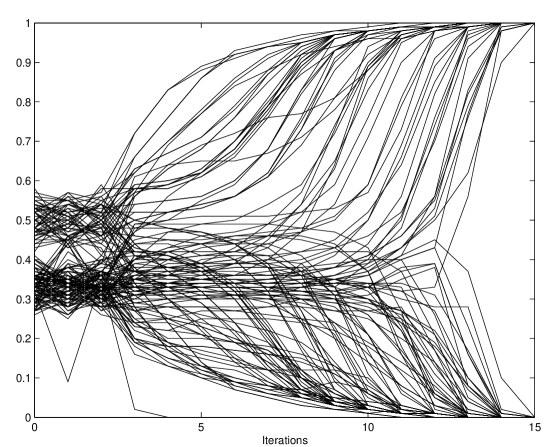
Figure 7: Evolution of neuron components $v_{ij}$ as the temperature is lowered for the template LD problem.

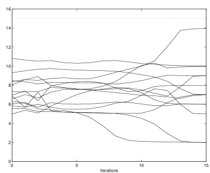
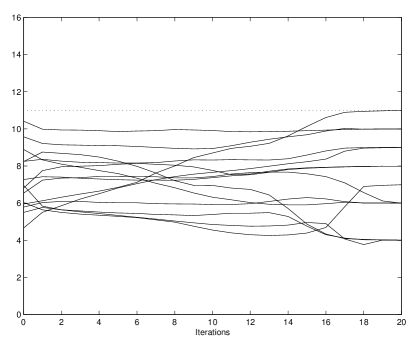
Figure 8: Evolution of $L_{ib}$ for all departure flights from the home base, $i$, for the template LD problem. The dotted lines denote $L^{\mbox{\footnotesize max}}_{\mbox{\footnotesize rot}}$.

When evaluating a solution obtained with the Potts approach, a check is done as to whether it is legal (if not, a simple post-processor tries to restores legality – this is only occasionally needed), then the solution quality is probed by measuring the excess waiting-time $R$,

$$R=\frac{T^{\mbox{\footnotesize wait}}_{\mbox{\footnotesize Potts}}-T^{\mbox{\footnotesize unr}}_{\mbox{\footnotesize wait}}}{\mbox{period}},$$ (33)

which is a non-negative integer for a legal solution.

For a given problem size, as given by the desired number of airports $N_{a}$ and flights $N_{f}$, a set of 10 distinct problems is generated. Each problem is subsequently reduced, and the Potts algorithm is applied to the resulting kernel problem. The solutions are evaluated, and the average $R$ for the set is computed. The results for a set of problem sizes ranging from $N_{f}\simeq 75$ to $1000$ are shown in tables 2 and 3; for the two template problems see table 4.

$N_{f}$	$N_{a}$	$<N^{\mbox{\footnotesize eff}}_{f}>$	$<N^{\mbox{\footnotesize eff}}_{a}>$	$<$ R $>$	$<$ CPU time $>$
75	5	23	8	0.0	0.0 sec
100	5	44	13	0.0	0.2 sec
150	10	46	14	0.0	0.1 sec
200	10	84	24	0.0	0.7 sec
225	15	74	22	0.0	0.4 sec
300	15	132	38	0.0	1.5 sec

Table 2: Average performance of the Potts algorithm for LD problems. The superscript “eff” refers to the kernel problem, subscripts “$f$” and “$a$” refer to respectively flight and airport. The averages are taken with 10 different problems for each $N_{f}$. $R$ is the excess waiting-time, and the CPU time refers to DEC Alpha 2000.

$N_{f}$	$N_{a}$	$<N^{\mbox{\footnotesize eff}}_{f}>$	$<N^{\mbox{\footnotesize eff}}_{a}>$	$<$ R $>$	$<$ CPU time $>$
600	40	280	64	0.0	19 sec
675	45	327	72	0.0	35 sec
700	35	370	83	0.0	56 sec
750	50	414	87	0.0	90 sec
800	40	441	91	0.0	164 sec
900	45	535	101	0.0	390 sec
1000	50	614	109	0.0	656 sec

Table 3: Average performance of the Potts algorithm for SMD problems. The averages are taken with 10 different problems for each size. Same notation as in table 2.

$N_{f}$	$N_{a}$	$<N^{\mbox{\footnotesize eff}}_{f}>$	$<N^{\mbox{\footnotesize eff}}_{a}>$	$<$ R $>$	$<$ CPU time $>$	type
189	15	71	24	0.0	0.6 sec	LD
948	64	383	98	0.0	184 sec	SMD

Table 4: Average performance of the Potts algorithm for 10 runs on the two template problems. Same notation as in table 2.

The results are quite impressive – the Potts algorithm has solved all problems, and with a very modest CPU time consumption, of which the major part is used in updating the $P$ matrix, using the fast method of eqs. (26, 27). The iteration time scales like $(N^{\mbox{\footnotesize eff}}_{f})^{3}\propto N_{f}^{3}$ with a small prefactor. This should be multiplied by the number of iterations needed – empirically between 20 and 40, independently of problem size.

9 Summary

We have developed a mean field Potts approach for finding good solutions to airline crew scheduling problems resembling real-world situations.

A key feature is the handling of global entities, sensitive to the dynamically changing “fuzzy” topology, by means of a propagator formalism. This is a novel ingredient in ANN-based approaches to resource allocation problems. Another important ingredient is the problem size reduction achieved by airport fragmentation and flight clustering, narrowing down the solution space by removing much of the sub-optimal part. This is done by exploiting the local properties of the corresponding unrestricted problems [1].

High quality solutions are consistently found throughout a range of problem sizes without having to fine-tune the parameters, with a time consumption scaling as the cube of the problem size. The performance of the Potts algorithm is probed by comparing to the unrestricted optimal solutions.

At first sight, the Potts algorithm appears difficult to implement in a parallel way with its global quantities. A concurrent implementations can be facilitated, however, by localizing all information.

The basic approach presented here is easy to adapt to other applications, in particular in communication routing [12].

Acknowledgements:

We thank Richard Blankenbecler for valuable suggestions on the manuscript. This work was in part supported by the Swedish Natural Science Research Council and the Swedish Board for Industrial and Technical Development.

Appendix Appendix A. A Toy Example

In this Appendix we define and analyze a small toy example with five airports, that is used throughout this paper to illustrate the various steps. When exploring the performance of the algorithm, much larger problems are of course involved (see Section 7).

The toy problem is specified in table A1, where a period of 10080 is assumed.

Flight	Dep. airport	Arr. airport	Dep. time	Arr. time
1	HB	B	0	500
2	B	C	1000	1300
3	C	D	1500	1850
4	D	E	4300	4870
5	E	HB	5100	5500
6	HB	B	1500	2000
7	B	D	2200	2800
8	D	HB	3500	4100
9	HB	B	6000	6500
10	B	D	7000	7500
11	D	HB	8000	8250

Table A1: Toy problem specification.

An illustration is shown in fig. 1.

Fragmentation and clustering with flight duration times and the number of legs added together gives the structures shown in fig. 3b and table A2. The corresponding kernel problem is shown in fig. 4 with the effective flights relabeled according to table A2.

Comp. flight	Leg-count	Legs	Dep. airport	Arr. airport	Dep. time	Arr. time
1	3	1-2-3	HB	D1	0	1850
2	2	4-5	D1	HB	4300	5500
3	2	6-7	HB	D1	1500	2800
4	1	8	D1	HB	3500	4100
5	3	9-10-11	HB	HB	6000	8250

Table A2: Toy model description after fragmentation and clustering. The first column gives the composite flight label.

The total flight-time is 5070, and without restrictions, there are two solutions with minimum waiting-time, 5280. One consists in the rotations 1-2, 3-4, and 5 in terms of composite flights, i.e. 1-2-3-4-5, 6-7-8, and 9-10-11 in terms of the original flights. The corresponding rotation times are 5500, 2600 and 2250, respectively. The other has the rotations 1-4, 2-3, and 5 in terms of composite flights, i.e. 1-2-3-8, 6-7-4-5, and 9-10-11 in terms of proper flights, with the respective rotation times 4100, 4000, and 2250.

Appendix Appendix B. The Potts Algorithm

Initialization

The initial temperature $T_{0}$ is assigned a tentative value of $1.0$. If the averaged squared change of the neurons,

$$(\Delta v)^{2}=\frac{1}{\tilde{N}_{f}}\sum_{ij}(\Delta v_{ij})^{2}=\frac{1}{\tilde{N}_{f}}\sum_{ij}(v_{ij}(t+1)-v_{ij}(t))^{2},$$ (B1)

is larger than 0.2 after the first iteration, then the system is reinitialized with $T_{0}\rightarrow 2T_{0}$. If, on the other hand, it is smaller than 0.01 the system is reinitialized with $T_{0}\rightarrow T_{0}/2$. In eq. (B1) $\tilde{N}_{f}$ is the number of flights minus those departing from HB,

Each neuron ${\bf v}_{i}$ is initialized by assigning random values to its components $v_{ij}$ in the interval $0.8/K$ to $1.2/K$, where $K$ is the number of components of the Potts neuron. The neuron is then normalized by dividing each component by the component sum.

Subsequently, $P_{ij}$, $T_{ij}$ and $L_{ij}$ are initialized consistently with the neuron values.

The following iteration is repeated, until one of the termination criteria (see below) is fulfilled:
Iteration
• For each airport (in random order) do: 1. For each arrival flight $i$, do: (a) Update ${\bf v}_{i}$ (eqs. (11,23)) (b) Update ${\bf P}$ (eq. (26) 2. Correct the neuron matrix by doing the following $N_{\mbox{\footnotesize norm}}$ times: (a) Normalize the columns of v, corresponding to local departures. (b) Normalize the rows of v, corresponding to local arrivals. • Decrease the temperature: $T=kT$.
We have consistently used $k=0.9$ and $N_{\mbox{\footnotesize norm}}=2$.

Termination criteria

The updating process is terminated if

$$1/\tilde{N}_{f}\sum_{ij}v_{ij}^{2}>0.99\;\;\mbox{and}\;\;\max_{ij}(\Delta v_{ij})^{2}<0.01\;\;\mbox{and}\;\;\min_{ij}v_{ij}^{2}>0.8,$$ (B2)

or

$$1/\tilde{N}_{f}\sum_{ij}v_{ij}^{2}>0.8\;\;\mbox{and}\;\;(\Delta v)^{2}>0.000001\;\;\mbox{and}\;\;\max_{ij}(\Delta v_{ij})^{2}<0.01\;\;\mbox{and}\;\;\min_{ij}v_{ij}^{2}>0.8,$$ (B3)

or if the number of iterations exceeds 100.

Postprocessing

First, the final state of each neuron ${\bf v}_{i}$ is analyzed with respect to its implied choice, defined by its largest component. A check is done as to whether a proper rotation structure results. If this is not the case (which never happened for the problems studied here), one may e.g. rerun the algorithm with modified parameters.

Then, each rotation is checked for legality: If the rotation time or leg count exceeds the respective bound, a simple algorithm is employed to attempt to restore legality, by swapping flights between rotations. For the few cases ($\sim$ 5 %) where such a correction was needed for the problems studied here, this procedure always sufficed.

Appendix Appendix C. The Problem Generator

We have made two distinct problem generators, tuned to generate problems statistically resembling the LD or SMD templates. In both generators, a random problem with a specified number of airports and flights is generated as follows.

First, the flight-times between airports are chosen randomly from a distribution, based on the relevant template problem. Then, a flight schedule is built up in the form of legal rotations starting and ending at the home-base. The waiting-times between consecutively flights are chosen in a random fashion in the neighbourhood of $T^{\mbox{\footnotesize unr}}_{\mbox{\footnotesize wait}}/N_{f}$ for the corresponding template problem.

For a specified number of airports $N_{a}$ and flights $N_{f}$, the key steps take the following form.

Generator steps
• The airports are assigned distinct probabilities, designed to match the traffic distribution for the airports in the relevant template problem. • For each pair of airports, a distance (flight-time) is drawn from a predefined distribution. • While the number of generated flights is less than $N_{f}$:
Start a new rotation from HB, then for each leg do: 1. Choose its destination: – If the number of legs is less than $L_{0}$, draw the destination from a predefined distribution, where HB is chosen with a probability $\cal{P}_{\mbox{\footnotesize HB}}$. – Else force the destination to be HB, and begin a new rotation. 2. Pick the waiting-time from the predefined distribution. 3. Set the flight time according to the distance table, with some random deviation. • If any rotation time exceeds the limit, or if the solution does not end up at the unrestricted minimal waiting-time, generate a new problem.

The probability $\cal{P}_{\mbox{\footnotesize HB}}$ for choosing HB as a destination is for both problem types chosen to 0.25, except for the first leg, giving on the average 5 legs per rotation. For LD-problems, the maximum legcount $L_{0}$ is set to 15, while for the SMD problems it is set to 25.

References

- [1] M. Lagerholm, C. Peterson and B. Söderberg, “Statistical Properties of Unrestricted Crew Scheduling Problems”, LU TP 97-11 (submitted to Operations Research).
- [2] J.J. Hopfield and D.W. Tank, “Neural Computation of Decisions in Optimization Problems”, Biological Cybernetics 52, 141 (1985).
- [3] C. Peterson and B. Söderberg, “A New Method for Mapping Optimization Problems onto Neural Networks”, International Journal of Neural Systems 1, 3 (1989).
- [4] R. Durbin and D. Willshaw, “An Analog Approach to the Traveling Salesman Problem using an Elastic Net Method”. Nature 326, 689 (1987).
- [5] C. Peterson, “Parallel Distributed Approaches to Combinatorial Optimization Problems – Benchmark Studies on TSP”, Neural Computation 2,261 (1990).
-
[6]
C. Peterson and B. Söderberg,