Speckle from phase ordering systems

Abstract

The statistical properties of coherent radiation scattered from phase-ordering materials are studied in detail using large-scale computer simulations and analytic arguments. Specifically, we consider a two-dimensional model with a nonconserved, scalar order parameter (Model A), quenched through an order-disorder transition into the two-phase regime. For such systems it is well established that the standard scaling hypothesis applies, consequently the average scattering intensity at wavevector ${\bf k}$ and time $\tau$ is proportional to a scaling function which depends only on a rescaled time, $t\sim|{\bf k}|^{2}\tau$. We find that the simulated intensities are exponentially distributed, and the time-dependent average is well approximated using a scaling function due to Ohta, Jasnow, and Kawasaki. Considering fluctuations around the average behavior, we find that the covariance of the scattering intensity for a single wavevector at two different times is proportional to a scaling function with natural variables $\delta t=|t_{1}-t_{2}|$ and $\bar{t}=(t_{1}+t_{2})/2$. In the asymptotic large-$\bar{t}$ limit this scaling function depends only on $z=\delta t/\bar{t}\,^{1/2}$. For small values of $z$, the scaling function is quadratic, corresponding to highly persistent behavior of the intensity fluctuations. We empirically establish that the intensity covariance (for ${\bf k}\neq 0$) equals the square of the spatial Fourier transform of the two-time, two-point correlation function of the order parameter. This connection allows sensitive testing, either experimental or numerical, of existing theories for two-time correlations in systems undergoing order-disorder phase transitions. Comparison between theoretical scaling functions and our numerical results requires no adjustable parameters.

I Introduction

A scattering experiment, using neutrons or X-rays for example, is one of the most direct measures of the structure of materials. Naively, this comes about because in the Born approximation, which usually applies for X-rays and neutrons, the intensity in scattering measurements is proportional to the Fourier transform of a density-density correlation function. It is the wavelike properties of the scattering probe which produces the Fourier transform. For a deeper understanding of the relationship between scattering intensity and structure one must realize that this direct correspondence applies precisely only for coherent waves. Indeed, for conventional sources, a given point in the incident wave is only coherent within a small volume of neighboring points. This coherence volume has transverse dimensions determined by how parallel the wavefronts are and a longitudinal length determined by how monochromatic the wave is. In a standard scattering experiment the different coherence regions of the incident beam scatter independently. The intensity measured thus depends on an incoherent average over different regions of the scattering volume. By restricting the scattering volume of the sample to less than the coherence volume of the beam, one can eliminate this incoherent average, and thus learn more about the material’s structure. Of course, the experimental difficulty which arises is to obtain sufficient diffracted intensity to measure a signal. Recently, it has been demonstrated that coherent diffraction experiments can be performed with X-rays using high-brilliance synchrotron sources[1]. For coherent diffraction, the scattering from an inhomogeneous material displays a characteristic speckled scattering pattern. For instance, the random distribution of phase-ordering domains shown in Fig. 1 and discussed below, results in the speckle pattern shown in Fig. 2. As the domains change shape, the speckle pattern changes, and this time dependence of the speckle offers a unique method for studying the evolution of inhomogeneous materials.

Motivated by these advances in experimental techniques, we have undertaken a theoretical study of intensity fluctuations caused by scattering from a nonequilibrium system undergoing phase ordering by domain growth. When a disordered homogeneous material is rapidly brought to a new set of conditions, corresponding to the coexistence of two equilibrium phases, a spatial pattern of domains of the two phases develops [2]. This change of conditions is often accomplished by a rapid quench from a high temperature to a low one below a miscibility gap. The quench from a homogeneous state with local fluctuations creates a microstructure of interconnecting, interlocking domains through the kinetics of a first-order phase transition. As time goes on the domains grow, so as to minimize the area of the domain walls that separate the phases.

When the average domain size $R(\tau)$ at time $\tau$ is large compared to all other relevant lengths, except for the extent $L$ of the system itself, the system looks invariant if all lengths are measured in units of that domain size. In this case the structure of these many domains is said to “scale” with $R(\tau)$. Experimentally, the growing domain structure is often studied by means of the scattering intensity [3], whose width is proportional to the inverse of $R(\tau)$. When the average scattering intensity is scaled in units of this time-dependent length, one obtains the scattering function for late times in the form of a time-independent scaling function. The time-dependence then enters only through $R(\tau)$, which can typically be described in terms of an exponent $n$, such that $R\sim\tau^{n}$. This scaling hypothesis has been found to apply to a large range of systems, and to be unaffected by many of the microscopic details of specific materials. That is, the scaling function and the growth exponent $n$ are two features which are common to a large number of systems, collectively called a universality class. Universality classes for phase ordering by domain growth are delineated chiefly by the presence or absence of conservation laws. Indeed, many aspects of this nonequilibrium process can be described by relatively simple theoretical models. For example, for systems described by a nonconserved scalar order parameter, often called Model A [2], the growth exponent is found to be $n=1/2$. Systems included in this class are the Ising model with spin-flip dynamics, binary alloys undergoing an order-disorder transition, and some magnetic materials with uniaxial anisotropy. Model B [2] refers to systems in which the scalar order parameter is conserved, and the only growth mechanism is diffusion. Systems in this universality class have $n=1/3$ and include the conserved Ising model, as well as binary alloys undergoing phase separation.

In the present paper we investigate the time-dependent fluctuations around this scaling behavior, and we demonstrate how to study these fluctuations experimentally through analysis of the time-dependent scattering. The first theoretical study of such behavior is given in Ref. [4]. The scattering intensity is related to the Fourier transform of the order parameter $\psi({\bf r},\tau)$, the scalar field describing the inhomogeneity of a specific sample of the scattering material, by

$$I({\bf k},\tau)=|\hat{\psi}({\bf k},\tau)|^{2}\;,$$ (1)

where we ignore the proportionality constant for convenience. The average of $I({\bf k},\tau)$ over an ensemble of initial conditions is the structure factor,

$$S({\bf k},\tau)=\langle I({\bf k},\tau)\rangle\;.$$ (2)

Here, the ensemble average expresses the distinction between coherent scattering, given by $I$, and incoherent scattering, given by $S$. Fluctuations around the average scattering are the main topic of interest in this paper. The structure factor can also be expressed as the Fourier transform of the correlation function of $\psi({\bf r},\tau)$,

$$C({\bf r},\tau)=\langle\psi({\bf 0},\tau)\psi({\bf r},\tau)\rangle\;.$$ (3)

Because of these relationships, the scattering intensity and structure factor have been important tools for studying the dynamics of materials far from equilibrium. If a system is isotropic, then its average scattering properties depend only on the magnitude of the scattering wavevector, $|{\bf k}|=k$.

As mentioned above, scaling by the domain size $R\sim\tau^{n}$ implies that correlations are time independent when measured in units of $R$. Specifically, for an isotropic system, $C(r,\tau)=\overline{C}(r/R(\tau))$, where $\overline{C}(\overline{r})$ is one form of the scaling function. Fourier transformation gives the average scattering intensity in terms of another form of the scaling function, which depends only on a scaled time $t\propto\tau k^{1/n}$,

$$k^{d}S(k,\tau)=F_{1}(t)\;,$$ (4)

where $d$ is the spatial dimension of the scattering material. The specific form of $F_{1}(t)$ depends on the dynamic universality class.

As discussed above, when the scattering involves coherent radiation, $I({\bf k},\tau)$ is directly measured without self-averaging. The scattering from an inhomogeneous material displays a characteristic speckled scattering pattern much like the one in Fig. 2, which shows the squared norm of the Fourier transform of the configuration in Fig. 1. The intensity of each speckle in $I({\bf k},\tau)$ is due to correlations in the inhomogeneous sample, and $I-\langle I\rangle=I-S$ gives the fluctuations around the average scattering intensity.

For materials in equilibrium, deviations of $I$ around the structure factor are induced by thermal fluctuations in $\psi$. In fact, fluctuations in the speckle patterns from scattered laser light have been used as the standard basis of photon correlation experiments at wavelengths ranging from the ultraviolet to the infrared [5, 6]. With the advent of high-brilliance synchrotron photon sources, experiments involving coherent X-rays have become possible. For example, Brownian diffusion rates in gold colloids have been determined from the time required for a change in an X-ray speckle pattern [7, 8]. Speckle from coherent X-rays has also been used to study equilibrium fluctuations in Fe₃Al near an order-disorder transition [9], and in micellar block-copolymer systems [10]. X-rays can probe materials on much smaller length scales than is currently possible with lasers, and their greater penetration allows the study of optically opaque materials.

In the present paper, we present a theoretical study of fluctuations in the scattering intensity from a nonequilibrium system undergoing phase ordering by domain growth. For such systems the intensity fluctuates around a time-dependent structure factor [4, 11, 12]. The time evolution of the intensity at a specific wavevector for one particular quench can be normalized by the average behavior. A typical example of such a normalized time series, obtained from a simulation at zero temperature, is presented in Fig. 3. It is the correlations of such time series, averaged over many individual speckles and quenches, that can be used to study the pattern formation process in phase-ordering materials.

In Fig. 3 we also show a “Brownian” function which was constructed to have the same single-time probability density and an exponential two-time covariance with the same characteristic time as the normalized nonequilibrium scattering intensity. Qualitative differences are immediately evident in the two time series. The Brownian function fluctuates quickly, with large amplitude variations, while the intensity fluctuations produced by the phase-ordering system vary slowly, with markedly less variation in amplitude on short time scales [12]. This property of the nonequilibrium intensity fluctuations is called persistence [13], and it indicates a qualitative difference between the two-time correlation functions for the two processes [14].

For the remainder of this paper, we specialize to Model A as a simple model for systems undergoing phase ordering following a quench through a second-order order–disorder phase transition. Some preliminary numerical results from simulations less extensive than the ones used here were presented in Ref. [15].

The outline of the rest of this paper is as follows. Section II describes the details of our numerical approach, which uses a standard time-dependent Ginzburg-Landau equation with a nonconserved order parameter. In Sec. III the time-time covariance of individual speckle intensities is discussed, using analysis readily adaptable to experimental data. The equality between this covariance and the square of the two-time structure factor of the nonequilibrium material is argued in Sec. IV, and comparisons to specific two-time theories follow in Sec. V. There an analytic expression for the universal scaling form for the intensity covariance at late times is obtained. Finally, our results are summarized in Sec. VI.

II Method

The dynamics of speckle in ${\bf k}$-space were simulated by generating successive scattering patterns from a real-space simulation of the dynamics of phase ordering following a quench through an order-disorder phase transition. The configuration of the real-space system is described by a nonconserved scalar order-parameter field $\psi({\bf r},\tau)$, and its dynamics are governed by the following time-dependent Ginzburg-Landau equation,

$$\frac{\partial\psi({\bf r},\tau)}{\partial\tau}=-\Gamma\frac{\delta{\cal F}[\psi({\bf r},\tau)]}{\delta\psi({\bf r},\tau)}+\zeta({\bf r},\tau)\;.$$ (5)

The first term on the right-hand side of this Langevin equation corresponds to deterministic relaxation, with rate constant $\Gamma$, towards a minimum value of the free-energy functional ${\cal F}[\psi({\bf r},\tau)]$. Thermal noise, which we neglect, is modeled by the random variable $\zeta$, whose intensity is proportional to $\Gamma$ and temperature by virtue of a fluctuation-dissipation theorem [2]. We neglect $\zeta$ because the most important sources of noise here are the initial conditions, which give the random domain morphology. The main effect of thermal noise at low temperatures far below any critical point, is only to thermally roughen the domain walls.

We employ the standard Ginzburg-Landau-Wilson free energy [2],

$${\cal F}[\psi({\bf r},\tau)]=\int d{\bf r}\Bigg{[}-\frac{a}{2}\psi^{2}({\bf r},\tau)+\frac{u}{4}\psi^{4}({\bf r},\tau)+\frac{c}{2}|{\bf\nabla}\psi({\bf r},\tau)|^{2}\Bigg{]}\;.$$ (6)

For $a>0,$ the local part of the integrand in Eq. (6) represents a bistable potential, and the parameters of the model define an equilibrium field magnitude, $|\psi_{0}|=\sqrt{a/u}$, a thermal correlation length, $\xi_{0}=\sqrt{2c/a}$, and a characteristic evolution time, $\tau_{0}=(a\Gamma)^{-1}$. The model can be rescaled by choosing a new field $\tilde{\psi}=\psi/|\psi_{0}|$, a new length $\tilde{\bf r}=\sqrt{2}{\bf r}/\xi_{0}$, and a new time $\tilde{\tau}=\tau/\tau_{0}$. Dropping the tilde from the rescaled quantities for convenience, we get the rescaled dynamical equation,

$$\frac{\partial\psi({\bf r},\tau)}{\partial\tau}=\left(1+\nabla^{2}\right)\psi({\bf r},\tau)-\psi^{3}({\bf r},\tau)\;,$$ (7)

which has no adjustable parameters. Since thermal fluctuations are explicitly omitted in the simulation, the only randomness comes from the high-temperature state the system is in before the quench. This was implemented by an initial condition such that $\psi({\bf r},0)$ consists of independent random numbers uniformly distributed between $\pm 0.1$.

The simulations were conducted on square lattices with periodic boundary conditions, lattice constant $\Delta r=1\,$, and a system size of $L_{x}=L_{y}=L=1024$. The Laplacian in Eq. (7) was implemented using the eight-neighbor discretization [16, 17]

$$\nabla^{2}\psi=\frac{1}{2(\Delta r)^{2}}\Bigg{(}\sum\psi_{\rm NN}+\frac{1}{2}\sum\psi_{\rm NNN}-6\psi\Bigg{)}\;,$$ (8)

where $\psi_{\rm NN}$ are the four nearest neighbors of $\psi$ (along the lattice directions), and $\psi_{\rm NNN}$ are its four next-nearest neighbors (diagonally). A simple Euler integration scheme with $\Delta\tau=0.05$ was used to collect data up to a maximum rescaled time of $\tau=2000$ for $100$ separate sets of initial conditions.

Usually, the order parameter takes the values $\pm|\psi_{0}|$ everywhere except at the domain walls, which are negligibly thin compared to the domains themselves. After our rescaling, domain walls have a soft nonzero width of approximately $\sqrt{2}$. To minimize the effect of this nonzero, though small, width, we use a nonlinear mapping of the rescaled order parameter to $\pm 1$ before taking the Fourier transform. The transformed field, $\hat{\psi}$, is defined by

$$\hat{\psi}({\bf k},\tau)=\frac{1}{\sqrt{L^{d}}}\sum_{\bf r}{\rm sign}\,\Big{(}\psi({\bf r},\tau)\Big{)}e^{i{\bf k\cdot r}}\;,$$ (9)

where the fact that the lattice spacing is unity in all directions has been used. The Brillouin zone in two dimensions is defined by the discrete set of wavevectors, $k_{x}$, $k_{y}=2\pi j/L$ with $j\in\{0,\,\pm 1,\,\pm 2,\,\dots,\,\pm(L/2-1),\,L/2\}$. The scattering intensity $I({\bf k},\tau)=|\hat{\psi}({\bf k},\tau)|^{2}$ and its average over initial conditions is the time dependent structure factor, $S({\bf k},t)$, as described in Sec. I. To be consistent with the numerical integration, the magnitude of the scattering wavevector, $k({\bf k})$, is defined using the operator relation

$$-k^{2}({\bf k})\hat{\psi}({\bf k},\tau)=\frac{1}{\sqrt{L^{d}}}\sum_{\bf r}e^{i{\bf k\cdot r}}\nabla^{2}\psi({\bf r},\tau)\;.$$ (10)

Substituting the discrete version of the Laplacian from Eq. (8), one obtains for $d=2$

$$k^{2}({\bf k})=3-\cos{k_{x}}-\cos{k_{y}}-\frac{1}{2}\cos{(k_{x}+k_{y})}-\frac{1}{2}\cos{(k_{x}-k_{y})}\;.$$ (11)

This method has been used to calculate the magnitude of the wavevector for scaling structure factors and data binning. Because of lattice effects we consider only those wavevectors with $0<k({\bf k})\leq 0.75$.

In order to apply the scaling ansatz, one must know the characteristic length at time $\tau$. Often $R(\tau)$ is estimated from the structure factor, however we have found an analytic expression that works well. Indeed, one advantage of our numerical approach, as compared to Monte Carlo or cell dynamical simulations, is that we can test theories without using any free parameters. In particular, Ohta, Jasnow, and Kawasaki [18] found that the time dependence of the domain size obeyed $R(\tau)=\sqrt{4\rho_{d}\tau}$, with $\rho_{d}=(d-1)/d$. Furthermore, they found that the structure factor scaled, and they gave an explicit form for the scaling function $F_{1}(t)$. In comparison, the theory of Kawasaki, Yalabik, and Gunton [19] gives the same form of $F_{1}(t)$, but the factor $\rho_{d}$ does not appear in their result for $R(\tau)$. Our present simulations agree with the amplitude given by Ohta et al., and so we choose a scaled time $t$ given by

$$t({\bf k},\tau)=[kR(\tau)]^{2}=4\rho_{d}k^{2}\tau\;.$$ (12)

III Two-time Correlation Functions

A quantity to which experiments give ready access is the fluctuation in the speckle intensity as a function of time. The relationship between an individual speckle at two different times $\tau_{1}$ and $\tau_{2}$ is, on average, described by the intensity covariance,

$${\rm Cov_{k}}({\bf k},\tau_{1},\tau_{2})=\Big{\langle}I({\bf k},\tau_{1})I({\bf k},\tau_{2})\Big{\rangle}-\Big{\langle}I({\bf k},\tau_{1})\Big{\rangle}\Big{\langle}I({\bf k},\tau_{2})\Big{\rangle}\;.$$ (13)

For random systems, the covariance is maximum in the equal-time limit, $\tau_{1}=\tau_{2}$, and as the two measurement times become widely separated, the values of the intensity become stochastically independent and the covariance decays to zero. For this relaxational system, negative values are not expected. The scaling ansatz extended to this situation allows collapse of the covariance at different $({\bf k},\tau_{1},\tau_{2})$ by

$$k^{2d}{\rm Cov_{k}}(k,\tau_{1},\tau_{2})={\rm Cov}(t_{1},t_{2})$$ (14)

where ${\rm Cov}(t_{1},t_{2})$ is the scaling function for the covariance.

The simulated scattering intensities were analyzed in the following way. In Eq. (14), the ensemble average over initial conditions is scaled to the universal form. To make estimates of ${\rm Cov}(t_{1},t_{2})$ from the simulations, we changed the order of the averaging and used the single-simulation averages $M_{1}(t)$ and $M_{2}(t_{1},t_{2})$. $M_{1}(t)$ is the scaled intensity, $k^{d}I({\bf k},\tau)$, averaged over all pairs of $({\bf k},\tau)$ that map onto $t$, and $M_{2}(t_{1},t_{2})$ is the scaled product of the intensities at two different times, $k^{2d}I({\bf k},\tau_{1})I({\bf k},\tau_{2})$, averaged over all triples $({\bf k},\tau_{1},\tau_{2})$ that map onto $(t_{1},t_{2})$. Due to the large amount of data involved in the present study, samples for $M_{1}(t_{1})$, $M_{1}(t_{2})$ and $M_{2}(t_{1},t_{2})$ were accumulated in a two-dimensional structure of bins organized by a pair of variables related to $(t_{1},t_{2})$ as described below. After accumulation into the bins $(t_{1},t_{2})$, averaging over independent runs, i.e., over different initial conditions, was performed to further improve our statistics. These averages were then used to find the scaling function ${\rm Cov}(t_{1},t_{2})$. It should be noted that all the quantities used here are also readily obtained experimentally, except for two unknown proportionality constants that depend on details of the experimental system. One occurs in the equation for the scaled time, corresponding to $4\rho_{d}$ in Eq. (12). The other is the proportionality constant between the measured scattering intensity and the squared-norm of the Fourier transform of the order parameter, which we have ignored in Eq. (2). Neither of these should be a barrier to comparing our results to experiments.

The normalized analog of the covariance is the correlation function [20],

$${\rm Corr}({\bf k},\tau_{1},\tau_{2})=\frac{\Big{\langle}I({\bf k},\tau_{1})I({\bf k},\tau_{2})\Big{\rangle}-\Big{\langle}I({\bf k},\tau_{1})\Big{\rangle}\Big{\langle}I({\bf k},\tau_{2})\Big{\rangle}}{\sqrt{\Big{\langle}I^{2}({\bf k},\tau_{1})\Big{\rangle}-\Big{\langle}I({\bf k},\tau_{1})\Big{\rangle}^{2}}\sqrt{\Big{\langle}I^{2}({\bf k},\tau_{2})\Big{\rangle}-\Big{\langle}I({\bf k},\tau_{2})\Big{\rangle}^{2}}}\;.$$ (15)

${\rm Corr}({\bf k},\tau,\tau)$ is unity by construction, which removes the equal-time variations in the covariance as $\tau$ changes. Using the definitions of $M_{1}$ and $M_{2}$ above, the scaled version can be expressed as

$${\rm Corr}(t_{1},t_{2})=\frac{\Big{\langle}M_{2}(t_{1},t_{2})\Big{\rangle}-\Big{\langle}M_{1}(t_{1})\Big{\rangle}\Big{\langle}M_{1}(t_{2})\Big{\rangle}}{\sqrt{\Big{\langle}M_{2}(t_{1},t_{1})-\big{\langle}M_{1}(t_{1})\big{\rangle}^{2}\Big{\rangle}\Big{\langle}M_{2}(t_{2},t_{2})-\big{\langle}M_{1}(t_{2})\big{\rangle}^{2}\Big{\rangle}}}\;,$$ (16)

where $\langle\cdots\rangle$ denotes averaging over initial conditions as before. The contour plot of ${\rm Corr}$ in the $(t_{1},t_{2})$-plane, Fig. 4, shows how the correlations in individual speckle intensities decay. In this figure, the line ${\rm Corr}(t_{1},t_{2})=1$ extends along the diagonal. Moving away from that line, contours at values of $0.7$, $0.2$, $0.07$, and $0.02$ are shown. The scatter in the data is apparent for the last contour and becomes dominant for values of the correlation less than that. The striking feature of this figure is that the correlations increase in a nontrivial way as the phase-ordering continues. Thus, normalization by the time-dependent intensity is not sufficient to convert the speckle intensity to a stationary time series.

A more natural set of variables for studying this effect is $\bar{t}=(t_{1}+t_{2})/2$ and $\delta t=|t_{2}-t_{1}|.$ A constant value of $\bar{t}$ corresponds to a line perpendicular to the $t_{1}=t_{2}$ diagonal, while $\delta t$ measures the distance (in units of scaled time) away from the diagonal. The symmetry under exchange of $t_{1}$ and $t_{2}$ is retained. These variables were used for the binning of simulation results that produced Fig. 4, with data grouped into $250$ equally wide series for $0\leq\bar{t}\leq 1000$; each $\bar{t}$ series having $100$ equal-width bins with $0\leq\delta t\leq 2\bar{t}$.

The characteristic time difference, $\delta t_{c}$, required for the scaled intensity covariance, ${\rm Cov}(t_{1},t_{2})$, to decay to half its maximum value can be found as a function of $\bar{t}$. (The normalized correlation function, Corr$(t_{1},t_{2})$, does not decay to $1/2$ for small values of $\bar{t}$ .) Here, results for $M_{1}$ and $M_{2}$ for $0\leq\bar{t}\leq 2$ (in $10$ series, with $25$ bins within each series) were collected in addition to those previously mentioned. The value of $\delta t_{c}$ for each $\bar{t}$ was determined by linear interpolation, and the dependence of $\delta t_{c}$ on $\bar{t}$ is presented in log-log form in Fig. 5. In this figure, two asymptotic limits giving different algebraic relationships are obvious. For small values of $\bar{t}$ the relationship is linear, with the exponent determined by least squares being $1.00\pm 0.01$ for $\bar{t}<1$. At large values of $\bar{t},$ a least-squares fit for $\bar{t}>200$ gives an exponent of $0.49\pm 0.02$. The estimates of error here are from obtaining the exponents from different ranges of $\bar{t}$ in the simulation data; statistical error is an order of magnitude smaller than these estimates. The exponents we obtain are in good accord with theories discussed in Sec. V below, which give them to be 1 and $1/2$, respectively. However, the connection to theory requires some further justification, given in the following section.

IV Correlations in the Scattering Material

While experiments can measure time correlations readily through the covariance or the correlation of intensities, Cov or Corr, theories to date have made use of the two-point, two-time order-parameter correlation function, $C({\bf r},\tau_{1},\tau_{2})\equiv\langle\psi({\bf 0},\tau_{1})\psi({\bf r},\tau_{2})\rangle$. In this section we argue for, and empirically demonstrate, equality between the intensity covariance for ${\bf k}\neq 0$, which involves fourth moments of the order parameter, and the square of the spatial Fourier transform of the two-time order-parameter correlation function in our model.

The relationship is exact when $\hat{\psi}({\bf k})$ is a joint Gaussian random number, with its real and imaginary parts independent and Gaussian, as we will show below. However, establishing $\hat{\psi}({\bf k})$ to be approximately Gaussian in the present case is not trivial. Gaussian variables are a natural consequence of the central-limit theorem, which requires a large number of uncorrelated contributions to the variable (with some restrictions on the properties of the individual contributions). For example, in a disordered system in equilibrium, correlations exist only on the scale of a small length $\xi$, so a system of edge-length $L$ consists of on the order of $(L/\xi)^{d}$ independent, uncorrelated parts. Then the central-limit theorem applies, and $\hat{\psi}({\bf k})$ is a complex, Gaussian variable. For an ordered system in equilibrium, this argument applies to the fluctuations around the ordered state. The present nonequilibrium situation has some rough analogies to a disordered equilibrium state. At a given time, the average domain size is $R(\tau)$, and so the number of independent parts at a given time is approximately $(L/R(\tau))^{d}$, which can be large. It therefore seems reasonable to expect the central-limit theorem to apply, and indeed, we find empirically that $\hat{\psi}({\bf k})$ is Gaussian. However, unlike a disordered system, the distribution of domains of different sizes is broad in this case due to the initial long-wavelength instability and, furthermore, it is clear that domains interact as they grow. The degree to which this correlation is important is a nontrivial issue; below, we test it numerically and find these correlations to be negligible for the two-point quantities of interest in this work.

If $\hat{\psi}({\bf k})$ is Gaussian, it is straightforward to relate the intensity covariance ${\rm Cov_{k}}$ to the order-parameter correlation function $C$. Wick’s theorem can be used to decompose the intensity-intensity average as

$$\Big{\langle}I({\bf k},\tau_{1})I({\bf k},\tau_{2})\Big{\rangle} = \Big{\langle}\hat{\psi}({\bf k},\tau_{1})\hat{\psi}^{*}({\bf k},\tau_{1})\hat{\psi}({\bf k},\tau_{2})\hat{\psi}^{*}({\bf k},\tau_{2})\Big{\rangle}$$ (17)

$$= \quad\hphantom{+}\quad\Big{\langle}\hat{\psi}({\bf k},\tau_{1})\hat{\psi}^{*}({\bf k},\tau_{1})\Big{\rangle}\Big{\langle}\hat{\psi}({\bf k},\tau_{2})\hat{\psi}^{*}({\bf k},\tau_{2})\Big{\rangle}$$ (20)

$$\quad+\quad\Big{\langle}\hat{\psi}({\bf k},\tau_{1})\hat{\psi}^{*}({\bf k},\tau_{2})\Big{\rangle}\Big{\langle}\hat{\psi}^{*}({\bf k},\tau_{1})\hat{\psi}({\bf k},\tau_{2})\Big{\rangle}$$

$$\quad+\quad\Big{\langle}\hat{\psi}({\bf k},\tau_{1})\hat{\psi}({\bf k},\tau_{2})\Big{\rangle}\Big{\langle}\hat{\psi}^{*}({\bf k},\tau_{1})\hat{\psi}^{*}({\bf k},\tau_{2})\Big{\rangle}$$

$$= (1+\delta_{{\bf k},0})S^{2}({\bf k},\tau_{1},\tau_{2})+S({\bf k},\tau_{1})S({\bf k},\tau_{2})\;.$$ (21)

Here $S({\bf k},\tau_{1},\tau_{2})$ is the two-time structure factor corresponding to the two-point, two-time order-parameter correlation function

$$S({\bf k},\tau_{1},\tau_{2}) = \Big{\langle}\hat{\psi}({\bf k},\tau_{1})\hat{\psi}^{*}({\bf k},\tau_{2})\Big{\rangle}$$ (22)

$$= \int d{\bf r}e^{i{\bf k}\cdot{\bf r}}C({\bf r},\tau_{1},\tau_{2})\;.$$ (23)

For ${\bf k}\neq 0$, Eq. (21) can be rewritten as

$${\rm Cov_{k}}({\bf k},\tau_{1},\tau_{2})=S^{2}({\bf k},\tau_{1},\tau_{2})\;,$$ (24)

which equates the speckle intensity covariance with the square of the two-time structure factor of the system. Finally, the scaling ansatz defines a universal two-time form

$$F_{2}(t_{1},t_{2})=k^{d}S(k,\tau_{1},\tau_{2})$$ (25)

and

$${\rm Cov}(t_{1},t_{2})=F^{2}_{2}(t_{1},t_{2})\;.$$ (26)

Our numerical tests show that this equality holds well in these simulations for $k\neq 0$. In computer simulations, unlike scattering experiments, the two-time structure factor can be found directly using Eq. (22). Generally, the product $\hat{\psi}({\bf k},\tau_{1})\hat{\psi}^{*}({\bf k},\tau_{2})$ is a complex number, but the mean value of the imaginary part is zero, so the two-time structure factor is real valued. In our simulation data, the imaginary part of $S(k,\tau_{1},\tau_{2})$ is found to be zero, within our accuracy. Results for the real part at $\tau_{1}=25$ and $\tau_{2}=50$ are presented on a log-log scale in Fig. 6. The direct measurements of the two-time structure factor and the square-root of the intensity covariance agree quite well, except at very large values of $k$, where lattice effects are important.

Another consequence of our proposed decoupling, leading to the relationship between ${\rm Cov_{k}}$ and $S$, can be tested by simulation. When $\tau_{1}=\tau_{2}$, Eq. (24) is simply

$$\left\langle I^{2}({\bf k},\tau)\right\rangle-\left\langle I({\bf k},\tau)\right\rangle^{2}=\left\langle I({\bf k},\tau)\right\rangle^{2}\;,$$ (27)

and scaling can be applied to give $F_{1}(t)=F_{2}(t,t)=\sqrt{{\rm Cov}(t,t)}$. These are compared in Fig. 7, where the agreement is clearly quite good. As an aside, since the variance does not depend on the system size, Eq. (27) demonstrates that $I({\bf k},\tau)$ is a spatially non-self-averaging quantity [21]. Because of this, increasing the system size $L$ will not improve the estimate of $S({\bf k},\tau)$ given by a specific number of speckles. However, this is compensated by the fact that more independent speckles are available in a given range of ${\bf k}$ for each trial. Numerical results obtained by Shinozaki and Oono in a study of spinodal decomposition in three dimensions using the cell-dynamical method appear to be consistent with this result [22]. We also note that the normalization of the two-time intensity correlation function, Eq. (15), can be simplified using Eq. (27).

Equation (27) is a property of exponentially distributed variables, and to the extent that $\hat{\psi}({\bf k},\tau)$ is a Gaussian random number, $I({\bf k},\tau)$ will be an exponentially distributed random number. That is, the probability density for the normalized intensities, $s({\bf k},\tau)={I({\bf k},\tau)}/{S({\bf k},\tau)}$, should satisfy

$$P(s)=\exp{(-s)}\;,$$ (28)

independent of $({\bf k},\tau)$. The probability density $P(s)$ is normalized and has unit mean and standard deviation. Since $P(s)$ is identical for all values of $({\bf k},\tau)$, only one density function needs to be constructed. The results for all $0.024<k({\bf k})<0.75$ are presented for two times in log-linear form in Fig. 8. The histogram for $s$ is constructed with a bin size of $0.1,$ and the normalized intensity is found using the circular average of $I({\bf k},\tau)$ from the same trial. The lower bound on $k$ is chosen such that at least $20$ speckles contribute to this circular average. This histogram is accumulated over all $100$ trials and then normalized; for each histogram on the order of $10^{6}$ samples are available. The solid line is the expected density, $P(s)=\exp(-s)$. For the earlier time the probability density is exponential for all $s$. At the latest simulation time the density is exponential only for $s\lesssim 5$, with a higher than expected occurrence of speckles brighter than this. Still, less than $0.5\%$ of the points lie this far into the tail, and the deviation is inferred to be a finite-size effect because it becomes more pronounced as our simulation continues. This agrees with earlier simulations [15], in which increasing the system size eliminated the deviation. We believe this effect is an artifact of the periodic boundary conditions which allow stabilization of slab-like domain patterns [23], producing “frozen-in” interference patterns that remain bright while the average intensity steadily decreases. No $k$ dependence is found for $P(s).$

V Two-time theories

Two theoretical predictions for the two-point, two-time order-parameter correlation function exist, which will be described and then compared to our simulation results. The first is an analytic theory, due to Yeung and Jasnow [24], which is an extension of the analysis by Ohta, Jasnow and Kawasaki [18, 25]. The second theory, developed by Liu and Mazenko [26], is numerical. Both theories produce approximations for the two-point, two-time order parameter correlation function, $C({\bf r},\tau_{1},\tau_{2})$, in the asymptotic limit. These then give the structure factor through the general relation for the Fourier transform of a spherically symmetric function $f(r)$ in $d$ dimensions,

$$\int d{\bf r}e^{i{\bf k}\cdot{\bf r}}f(r)=(2\pi)^{\frac{d}{2}}k^{-d}\int_{0}^{\infty}du\,u^{\frac{d}{2}}\,J_{\frac{d}{2}-1}(u)\,f(u/k)\;,$$ (29)

where $J_{\nu}$ is a Bessel function of the first kind of order $\nu$.

In the scaling regime, where the domain-wall thickness can be ignored, the Yeung-Jasnow correlation function is [24],

$$C_{\rm YJ}(r,\tau_{1},\tau_{2})=\frac{2}{\pi}\arcsin\left[\left(\frac{2R(\tau_{1})R(\tau_{2})}{R(\tau_{1})^{2}+R(\tau_{2})^{2}}\right)^{\frac{d}{2}}\exp\left(\frac{-r^{2}}{R(\tau_{1})^{2}+R(\tau_{2})^{2}}\right)\right]\;.$$ (30)

With the previously defined variables, $\delta t=|t_{1}-t_{2}|$ and $\bar{t}=(t_{1}+t_{2})/2$, this yields

$$F_{2,\rm YJ}(\delta t,\bar{t}\,)=\frac{2}{\pi}(2\pi)^{\frac{d}{2}}\int_{0}^{\infty}du\,u^{\frac{d}{2}}\,J_{\frac{d}{2}-1}(u)\,{\rm arcsin}\Bigg{[}\Bigg{(}1-\Big{(}\frac{\delta t}{2\bar{t}}\Big{)}^{2}\Bigg{)}^{\frac{d}{4}}\exp{\Big{(}\frac{-u^{2}}{2\bar{t}}\Big{)}}\Bigg{]}\;,$$ (31)

Expansion of ${\rm arcsin}(x)$ about $x=0$, followed by term-wise integration, gives

$$F_{2,\rm YJ}(\delta t,\bar{t}\,)=\frac{2}{\pi}(2\pi)^{\frac{d}{2}}\bar{t}\,^{\frac{d}{2}}\sum_{j=0}^{\infty}\frac{(2j)!\,\left(1-\left(\frac{\delta t}{2\bar{t}}\right)^{2}\right)^{\frac{d(2j+1)}{4}}}{2^{2j}(j!)^{2}(2j+1)^{\frac{d+2}{2}}}\exp{\left(-\frac{\bar{t}}{2(2j+1)}\right)}\;.$$ (32)

This infinite series is convergent for all physical values of $\delta t$ and $\bar{t}$; however, its terms are in general nonmonotonic in $j$. Only as one or both of the scaled times $t_{1}$ and $t_{2}$ approaches zero, is the series well approximated by the $j$=0 term. The asymptotic early-time form,

$$F_{2,\rm YJ}(\delta t,\bar{t}\,)\approx\frac{2}{\pi}(2\pi)^{\frac{d}{2}}\Bigg{(}1-\Big{(}\frac{\delta t}{2\bar{t}}\Big{)}^{2}\Bigg{)}^{\frac{d}{4}}\bar{t}\,^{\frac{d}{2}}\exp{\Big{(}-\frac{\bar{t}}{2}\Big{)}}\;,$$ (34)

is therefore a good approximation to Eq. (31) only in the very restricted region,

$$0\leq 1-\left(\frac{\delta t}{2\bar{t}}\right)^{2}\ll 6^{\frac{2}{d}}\,3\exp\left(\frac{-2\bar{t}}{3d}\right)\;,$$ (35)

near the $t_{1}$ and $t_{2}$ axes or the origin.

A more useful, analytical result is obtained in the limit of large $\bar{t}$ and small $\delta t$. Then, the largest terms in the series occur in a relatively wide range of $j$ near $\bar{t}/2(d+3)$. For large $\bar{t}$, the exponential factors in Eq. (32) suppress the small-$j$ terms. The series can then be converted to an integral, and the factorials can be approximated by Stirling’s formula to give

$$F_{2,\rm YJ}(\delta t,\bar{t}\,)\approx\pi^{\frac{d-3}{2}}4^{\frac{d+1}{2}}\bar{t}\,^{-\frac{1}{2}}\int_{0}^{\infty}dw\,w^{\frac{d-1}{2}}\left(1-\left(\frac{\delta t}{2\bar{t}}\right)^{2}\right)^{\frac{\bar{t}d}{8w}}\exp{(-w)}\;.$$ (36)

The identity $\lim_{m\rightarrow\infty}(1-x/m)^{m}=\exp(-x)$ is used to obtain the explicitly integrable form,

$$F_{2,\rm YJ}(z,\bar{t}\,)\approx\pi^{\frac{d-3}{2}}4^{\frac{d+1}{2}}\bar{t}\,^{-\frac{1}{2}}\int_{0}^{\infty}dw\,w^{\frac{d-1}{2}}\exp\left[-\left(\frac{z^{2}d}{32w}+w\right)\right]\;,$$ (37)

where $z=\delta t/\sqrt{\bar{t}}$. We note that the full Yeung-Jasnow result, Eq. (31), as well as the early-time approximation, Eq. (34), depends on $\delta t$ only through the scaling combination $\delta t/\bar{t}$. However, in the asymptotic late-time approximation, Eq. (37), the natural scaling combination is $z=\delta t/\sqrt{\bar{t}}$. As we shall see below, this analytical result is in excellent agreement with our numerical simulations. Equation (37) is readily integrated to yield the explicit large-$\bar{t}$ asymptotic scaling function,

$$\bar{t}\,^{\frac{1}{2}}F_{2,\rm YJ}(z,\bar{t}\,)\approx\pi^{\frac{d-3}{2}}2^{\frac{d+3}{2}}\Bigg{(}z\sqrt{\frac{d}{8}}\Bigg{)}^{\frac{d+1}{2}}K_{\frac{d+1}{2}}\Bigg{(}z\sqrt{\frac{d}{8}}\Bigg{)}\;,$$ (38)

where $K_{n}$ is a modified Bessel function of the second kind. The right-hand side of this equation depends only on $z$. In this large-$\bar{t}$ limit, the asymptotic forms of this scaling function with respect to $z$ are

$$\bar{t}\,^{\frac{1}{2}}F_{2,\rm YJ}(z,\bar{t}\,)=\left\{\begin{array}[]{ll}\pi^{\frac{d-3}{2}}\Gamma\Big{(}\frac{d+1}{2}\Big{)}4^{\frac{d+1}{2}}\Big{(}1-\frac{1}{16}\frac{d}{d-1}z^{2}\Big{)}&{\rm for}\;\;z\ll 1\\ \pi^{\frac{d-2}{2}}2^{\frac{d+2}{2}}\Big{(}z\sqrt{\frac{d}{8}}\,\Big{)}^{\frac{d}{2}}\exp{\Big{(}-z\sqrt{\frac{d}{8}}\,\Big{)}}&{\rm for}\;\;1\ll z\ll 2\sqrt{\bar{t}}\end{array}\right.\;.$$ (39)

The first line of this equation is exact for $z=0$, where it gives the asymptotic Porod-tail limit of the Ohta-Jasnow-Kawasaki result for $t^{1/2}F_{1}(t)$. Note that, in the limit $\delta t=2\bar{t}$, the second line gives a nonzero value, in contrast to the proper result given in Eq. (34). When $z$ is on the order of $\sqrt{\bar{t}}$, $F_{2,\rm YJ}$ diverges from the small-$z$ approximation given in Eq. (39).

A nonrigorous scaling argument [28] suggests that the order-parameter correlation function should depend on wavevector and time through $k|R(\tau_{1})-R(\tau_{2})|\propto\delta t/\bar{t}\,^{(1-n)}$, when $\delta t\ll\bar{t}$. The scaling variable $z$ obtained above is consistent with this since $n=1/2$ for Model A. In fact, the $z=\delta t/\bar{t}\,^{(1-n)}$ result is obtained in the asymptotic large-$\bar{t}$ limit if one repeats the above calculation for general $n$, considering the Yeung-Jasnow form for the correlation function, Eq. (30), simply as an integrable approximation valid for small $r$.

The second theory for two-time correlations in Model A is due to Liu and Mazenko [26]. It is an extension of a theory developed by Mazenko [27] to predict the universal part of the two-point, one-time scaled order-parameter correlation function $\overline{C}(r/R(\tau))$. The heart of the Liu-Mazenko theory is the scaling ansatz

$$C\Big{(}{\bf r},\tau_{1},\tau_{2}\Big{)}=\overline{C}_{\rm LM}\Big{(}r/R(\tau_{2}),\tau_{2}/\tau_{1}\Big{)}$$ (40)

and the partial differential equation

$$\frac{\partial\overline{C}_{\rm LM}({\bf x},\tau^{\prime})}{\partial\tau^{\prime}}=\nabla_{x}^{2}\overline{C}_{\rm LM}({\bf x},\tau^{\prime})+2{\bf x}\cdot{\bf\nabla}_{x}\overline{C}_{\rm LM}({\bf x},\tau^{\prime})+\frac{1}{\mu^{*}}\tan{\Big{(}\frac{\pi}{2}\overline{C}_{\rm LM}({\bf x},\tau^{\prime})\Big{)}}\;.$$ (41)

In Eq. (41), $\overline{C}_{\rm LM}$ is considered a function of the rescaled variables ${\bf x}={\bf r}/(2\sqrt{\tau})$ and $4\tau^{\prime}=\ln{(\tau_{2}/\tau_{1})}$. Note that these definitions are in terms of the physical quantities, but the connections to the rescaled variables used in this work are straightforward. We have found numerical solutions in terms of Liu and Mazenko’s units, which we then converted so that all results shown here are in terms of the rescaling given in Section II. The Mazenko theory for one-time correlations [27] serves to provide input into the Liu-Mazenko model through the scaled order-parameter correlation function $\overline{C}_{\rm M}(x)=\overline{C}_{\rm LM}(x,\tau^{\prime}$=0) and the numerically obtained eigenvalue $\mu^{*}$. Since the system is assumed isotropic, Eq. (41) can be reduced to a single partial differential equation in terms of a radial distance $x$ and the logarithmic time ratio $\tau^{\prime}$.

The scaled order-parameter correlation function in the Liu-Mazenko theory is normalized to $\overline{C}_{\rm LM}(0,0)=1$, which causes the tangent term in Eq. (41) to diverge. Use of the transformation $G=\sin{(\pi\overline{C}_{\rm LM}/2)}$ leads to the small-time solution

$$\overline{C}_{\rm LM}(0,\tau^{\prime})=\frac{2}{\pi}{\rm arcsin}{\Bigg{(}\exp{\Bigg{(}-\frac{\pi}{2\mu^{*}(d-1)}\tau^{\prime}\Bigg{)}}\Bigg{)}}\;.$$ (42)

This solution is only needed to avoid numerical difficulties at $x=0$ for the first time increment. Aside from this, Eq. (41) can be solved numerically using a finite differencing scheme that is implicit with respect to the derivatives, but evaluates the tangent term explicitly. Using $\Delta x=0.01\mu^{*}$ and $\Delta\tau^{\prime}=10^{-5}$ we have reproduced Fig. 1 of Ref. [26]. In addition, the exponent for the autocorrelation $\overline{C}_{\rm LM}(0,\tau^{\prime})$ (which will be discussed later) is recovered. The Liu-Mazenko results can be compared to the theory presented here by taking $\bar{t}$ to be a parameter and noting that $\delta t=2\bar{t}\tanh{(2\tau^{\prime})}$. The two-time structure factor predicted by the Liu-Mazenko theory, found using the Fourier transform in Eq. (29), is

$$F_{2,\rm LM}(\delta t(\bar{t},\tau^{\prime}),\bar{t}\,)=(2\pi)^{\frac{d}{2}}\Bigg{(}\frac{2\bar{t}}{\rho_{d}(1+\exp{(-4\tau^{\prime})})}\Bigg{)}^{\frac{d+2}{4}}\times$$ (44)

$$\int_{0}^{\infty}dx\,x^{\frac{d}{2}}J_{\frac{d}{2}-1}{\Bigg{(}x\sqrt{\frac{2\bar{t}}{\rho_{d}(1+\exp{(-4\tau^{\prime})})}}\Bigg{)}}\overline{C}_{\rm LM}(x,\tau^{\prime})\;,$$

where the scaling function $\overline{C}_{\rm LM}(x,\tau^{\prime})$ itself depends on $d$.

The two-point, two-time order-parameter correlation functions predicted by the two theories can be compared directly with our simulation, without adjustable parameters. Both theories describe the data well in some instances, and poorly in others. Our results are presented in Fig. 9 for $\tau_{1}=100$ and $\tau_{2}=200$. Data from our simulation are circularly averaged with bins of width one in the rescaled distance units, then averaged over 80 trials. The agreement between the Yeung-Jasnow theory and our simulation is quite good for this choice of times, while the Liu-Mazenko result is only qualitatively correct.

For larger separations in time, the Yeung-Jasnow theory does not work as well, most noticeably in predicting the autocorrelation function,

$$A(\tau_{1},\tau_{2})\equiv\langle\psi({\bf r},\tau_{1})\psi({\bf r},\tau_{2})\rangle\;,$$ (45)

which is equivalent to $C({\bf r=0},\tau_{1},\tau_{2})$. Fisher and Huse [29] have argued that for $\tau_{2}\gg\tau_{1}$ the autocorrelation obeys the power-law

$$A(\tau_{1},\tau_{2})\sim[{R(\tau_{1})}/{R(\tau_{2})}]^{\lambda}$$ (46)

for late times. (Note that, since $R\propto\tau^{n}$, the variables used in this paper give $\ln\big{[}R(\tau_{1})/R(\tau_{2})\big{]}=-2n\tanh^{-1}\delta t/2\bar{t}$.) Fisher and Huse give physical arguments for $d/2\leq\lambda\leq d$. They point out that $\lambda=1$ for the $d=1$ Glauber model and conjecture that $\lambda=5/4$ for the two-dimensional spin-flip Ising model. In the limit $\tau_{2}\gg\tau_{1},$ the Yeung-Jasnow theory gives $\lambda=d/2,$ as is easily seen by setting $r=0$ in Eq. (30). The Liu-Mazenko theory yields $\lambda\approx 1.2887$ and $1.6726$ for two and three dimensions, respectively [26]. Cell-dynamical simulations performed by Liu and Mazenko [26] gave $\lambda=1.246\pm 0.02$ for $d=2.$ A recent experiment [30] found $\lambda=1.246\pm 0.079$ for a two-dimensional nematic liquid crystal using video techniques. For our simulations we measured $A(\tau_{1},\tau_{2})$ for several values of $\tau_{1}.$ The results are presented on a log-log scale versus $\tau_{2}/\tau_{1}$ in Fig. 10. [In this measurement we did not employ the nonlinear transformation $\psi\rightarrow{\rm sign}(\psi)$. This accounts for the fact that $A(\tau_{1},\tau_{1})<1$, but does not otherwise seem to affect the results.] In the figure, the data appear to support a power-law decay at the latest time, and the exponent found by fitting the $48$ points $\tau_{2}>1800$ for $\tau_{1}=20$ is $\lambda\approx 1.24$, which is in good agreement with the experiment and the simulations by Liu and Mazenko. However, the local effective value of $\lambda$, $\lambda_{\rm eff}=2d\ln A/d\ln(\tau_{1}/\tau_{2})$, which is shown vs. $\tau_{2}/\tau_{1}$ in the inset in Fig. 10, does not show a clear convergence to an asymptotic limit, especially for larger values of $\tau_{1}$. Here $\lambda_{\rm eff}$ is obtained as a three-point finite-difference estimate around $\tau_{2}$, but estimates that smooth the data over wider intervals yield similarly irregular results. The estimates of $\lambda$ obtained from our present simulations are thus somewhat uncertain. However, the Yeung-Jasnow prediction, $\lambda=1$, is clearly violated.

The predictions of the two theories for the two-time structure factor are compared to our simulation data in Fig. 6. The Liu-Mazenko theory is in semi-quantitative agreement with our simulations at small $k,$ but falls off much more rapidly at large $k$. In addition the shoulder present both in our simulation result and in the Yeung-Jasnow theory is absent in the Liu-Mazenko result. The Yeung-Jasnow theory agrees much better with our simulation, although it does not fall off as fast at large $k$, and its overestimation around the shoulder is seen consistently throughout our simulations.

The prediction for the characteristic scaled time separation, $\delta t_{c}$, defined in Sec. III, for both theories is compared to our simulation results in Fig. 5. All three agree that $\delta t_{c}=\tilde{D}_{d}\bar{t}$ for small $\bar{t}$. Least-squares fits give $\tilde{D}_{2}=1.36\pm 0.02$ for our simulation, $\tilde{D}_{2}=1.325\pm 0.002$ and $\tilde{D}_{3}=1.633\pm 0.006$ for Yeung-Jasnow, and $\tilde{D}_{2}=1.00\pm 0.02$ for Liu-Mazenko. At large $\bar{t}$, the $\delta t_{c}=D_{d}\bar{t}\,^{1/2}$ behavior of the Yeung-Jasnow approach results naturally from Eq. (38). This equation can be solved numerically to find $D_{2}\approx 2.156$ and $D_{3}\approx 2.187$ in two and three dimensions, respectively. Our simulation results give $D_{2}=2.12\pm 0.01.$ The value of $\bar{\tau}$ separating the two scaling behaviors corresponds quantitatively to the value for which the first term no longer dominates the series expansion of the Yeung-Jasnow result, given by the relation (35). The agreement between the Yeung-Jasnow theory and our simulation is quite remarkable. On the other hand, for $\bar{t}$ not small the Liu-Mazenko theory crosses over to a region where $\delta t_{c}$ is independent of $\bar{t}$ and then into another linear region; neither of these relationships is seen in our simulations.

The analytic expression for the universal form of the two-time structure factor deduced from the Yeung-Jasnow theory for large $\bar{t}$ is given in Eq. (38). It is tested for several values of $\bar{t}$ in Fig. 11, which shows good collapse of the simulation data for $\bar{t}{\rm Cov}(\delta t,\bar{t}\,)$ in terms of the scaling variable $z=\delta t/\bar{t}\,^{1/2}$. The data also agree quite well with the Yeung-Jasnow scaling function, $\bar{t}F^{2}_{2,{\rm YJ}}$ for $z<5$. Indeed, the slow quadratic decay of correlations near $z=0$ is another signature of persistence in the phase-ordering system. In contrast, Brownian fluctuations give exponential decay from $\delta t=0$. The agreement with the Yeung-Jasnow theory is remarkable since the scaling of the simulation data uses an analytic expression for the characteristic length, and no adjustable parameters are employed.

VI Conclusions

Using both numerical and analytic methods, we have investigated time-time correlations in the scattering intensity for a two-dimensional system undergoing an order-disorder transition. The correlations are found to obey scaling in terms of the variables $\delta t=|t_{2}-t_{1}|$ and $\bar{t}=(t_{1}+t_{2})/2.$ In the large $\bar{t}$ limit, the correlation data collapse onto a universal curve which is a function only of $\delta t/\sqrt{\bar{t}}.$

We argue for, and establish numerically, an exponential distribution for the scattering intensity, Eq. (28), and equality between the scattering intensity covariance and the square of the two-time structure factor of the order parameter, Eq. (24), for ${\bf k}\neq 0$. We use this equality to test theories for the two-time structure factor due to Yeung and Jasnow, and Liu and Mazenko. Both theories describe the data well in some instances, and poorly in other cases. The Yeung-Jasnow theory is very similar to our simulation results, so long as $\delta t$ is not too large. For $\tau_{2}\gg\tau_{1}$, the Liu-Mazenko theory gives a better estimate for the autocorrelation exponent $\lambda$. For large $\bar{t}$, however, the Liu-Mazenko theory does not show the same scaling as our simulation results, where the Yeung-Jasnow theory compares quantitatively well.

Our numerical simulations indicate that a definitive experimental treatment of time-correlations during an order-disorder transition is possible by intensity-correlation spectrometry of scattering speckle. Analysis of experimental correlation data should be similar to the procedures discussed for the simulation data in Sec. III. For non-conserved systems, the experimental scaling function should be well approximated by Eq. (34), for small $k$, with one adjustable parameter for each axis. With a similar adjustable parameter scheme, the scaling function should be described by Eq. (38) for data in the Porod tail.

Finally, we expect that the equality between the intensity covariance and the squared two-time structure factor also occurs in other phase-ordering systems; in particular, we expect that it occurs for conserved systems. That would allow the experimental study of, for example, time correlations in binary alloys undergoing phase separation by spinodal decomposition, which are representative of Model B. Indeed, preliminary numerical work we have done indicates this. Experiments on such systems would be of considerable value.

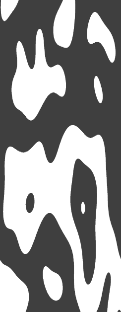
FIG. 1.: A typical configuration of domains, taken from one of the simulations reported here. Here all systems are $1024\times 1024$, and this picture is for the latest simulation time, $\tau=2000$.

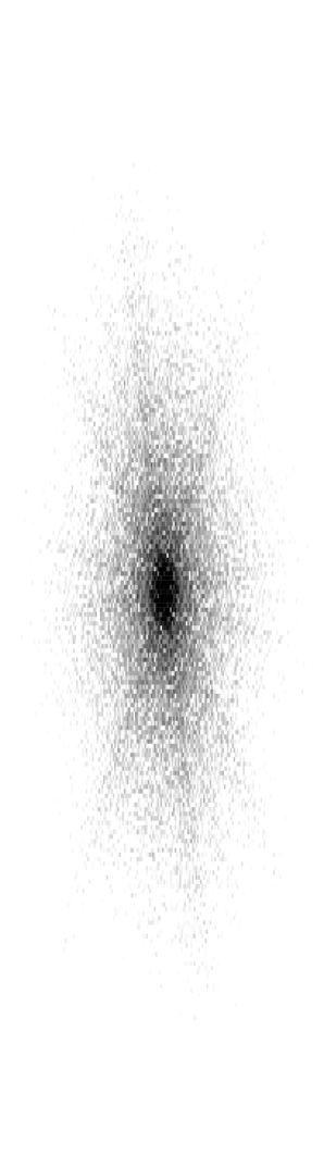
FIG. 2.: Example of the speckled scattering intensity; this pattern corresponds to the domain structure shown in Fig. 1. The intensity is shown on a logarithmic scale with darker shades indicating brighter speckles. This is a $200\times 200$ section from the full $1024\times 1024$ pattern with the ${\bf k}=0$ origin at the center of the figure. Speckles do not shift in $\bf k$-space, but their intensities fluctuate strongly around the $({\bf k},\tau)$-dependent average value. The rays are present in individual patterns, but are not correlated between trials.

FIG. 3.: Time evolution of the scattering intensity at one wavevector for one quench to zero temperature. The intensity has been normalized by the time-dependent structure factor determined over all 100 simulations considered here. The dotted line is a synthetic “Brownian” function constructed to have an exponential single-time probability density and an exponential two-time covariance with a characteristic time corresponding to that of the simulated intensity. Compared to the “Brownian” function, the persistence of the scattering intensity is apparent [13, 14].

FIG. 4.: Contour plot of the scaled two-time intensity correlation function, Corr$(t_{1},t_{2})$. The correlation at $t_{1}=t_{2}$ is unity by construction. The contours moving away from this diagonal are at $0.7$, $0.2$, $0.07$, and $0.02$. The figure shows that the speckle intensity stays correlated for larger values of $\delta t=|t_{2}-t_{1}|$ as $\bar{t}=(t_{1}+t_{2})/2$ increases.

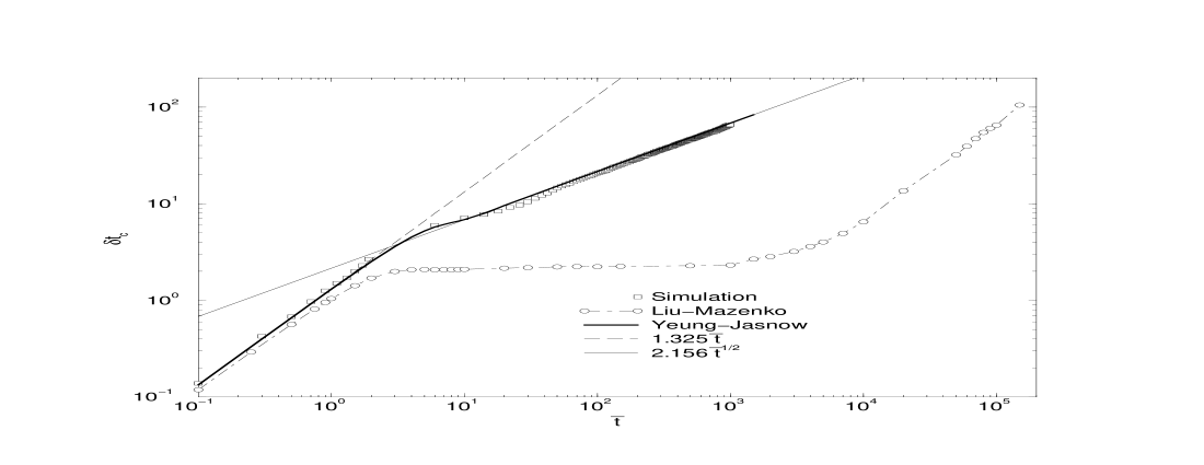
FIG. 5.: The characteristic decay time difference, $\delta t_{c},$ as a function of $\bar{t}=(t_{1}+t_{2})/2.$ Power-law behavior is seen at small and large values of $\bar{t}.$ Least-squares fits to the simulation data yield a linear relationship at small $\bar{t}$ and $\delta t_{c}\sim\bar{t}\,^{\alpha}$ with $\alpha\approx 1/2$ at large $\bar{t}$. The heavy solid line is the analytic prediction of the Yeung-Jasnow theory. The broken line is its small-$\bar{t}$ limit $\delta t_{c}\approx 1.325\bar{t}$, and the light solid line is the large-$\bar{t}$ approximation $\delta t_{c}\approx 2.156\sqrt{\bar{t}}$. The the $\bar{t}$ associated with the change in behavior agrees well with Eq. (35). The results of the Liu-Mazenko theory are represented as circles connected by a dot-dashed line; least-squares fits show them to be nearly linear at both small and large $\bar{t}$.

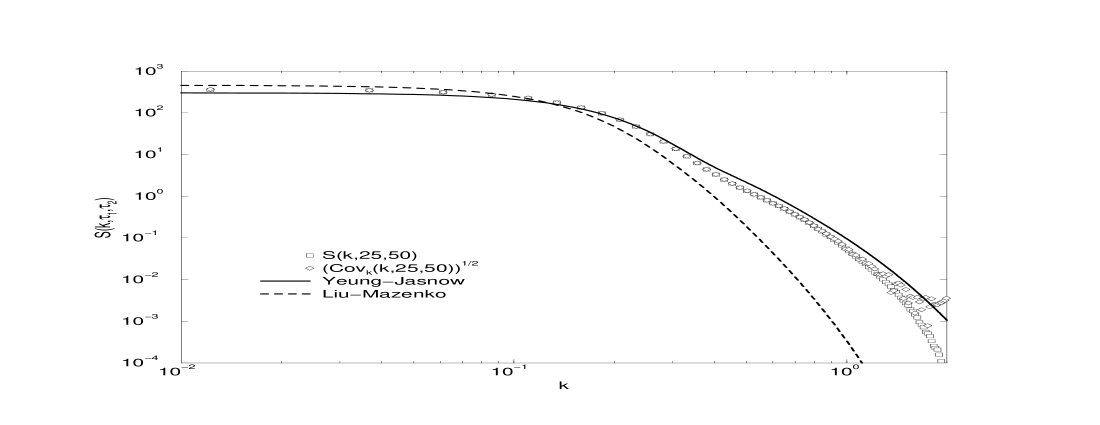
FIG. 6.: The two-time structure factor for $\tau_{1}=25$ and $\tau_{2}=50$. The simulation results are found directly as $S(k,\tau_{1},\tau_{2})$ (squares), and indirectly as $\sqrt{{\rm Cov_{k}}(k,\tau_{1},\tau_{2})}$ (diamonds). The Liu-Mazenko theory agrees semi-quantitatively at small $k.$ The Yeung-Jasnow theory agrees much better, even reproducing the second shoulder qualitatively.

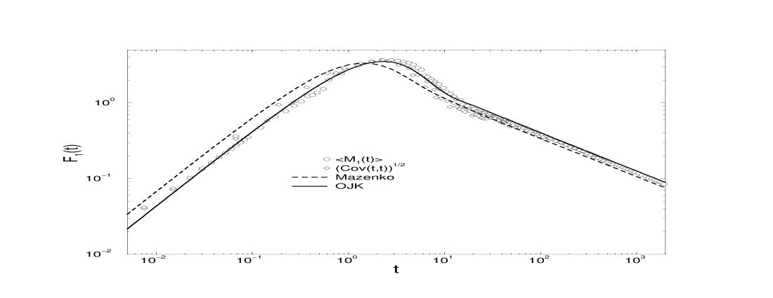
FIG. 7.: Estimates of the scaling function for the structure factor, $F_{1}(t)$, obtained from the simulation data using the average scaled scattering intensity, $\langle M_{1}(t)\rangle$ (circles), and the square-root of its variance, $\sqrt{{\rm Cov}(t,t)}$ (diamonds). The agreement between the two measurements is a direct consequence of the intensity being an exponentially distributed random variable. The forms obtained from the Yeung-Jasnow (solid line) and Mazenko (dashed line) theories are also included.

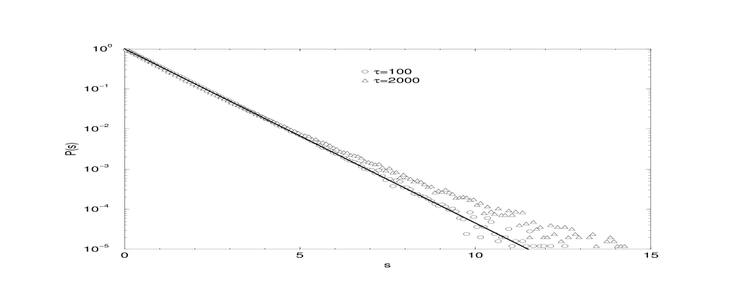
FIG. 8.: The probability density of the normalized speckle intensity, $s=I({\bf k},\tau)/S({\bf k},\tau)$, for $\tau=100$ (circles) and $\tau=2000$ (triangles). The solid line is the theoretical density of an exponentially distributed random variable. The deviation at large $s$ of the latest time result is due to finite-size effects.

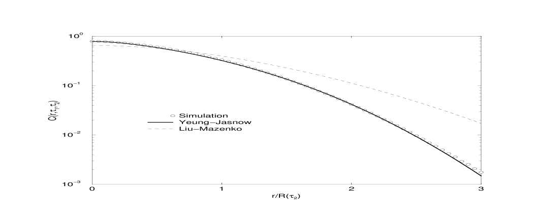
FIG. 9.: The two-time correlation function $C(r,\tau_{1},\tau_{2})$ with $\tau_{1}=100$ and $\tau_{2}=200$ presented on a semi-log scale. The characteristic length $R(\tau_{2})$ is determined analytically as described in the text. The agreement between the simulation (circles) and the Yeung-Jasnow theory (solid line) is quite good for this choice of parameters; the Liu-Mazenko theory (dashed line) is noticeably different. The agreement between simulations and Yeung-Jasnow is not as good for larger time separations.

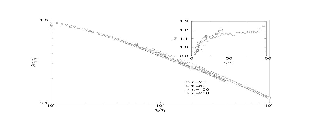
FIG. 10.: The autocorrelation function $A(\tau_{1},\tau_{2})$. A least-squares fit for $\tau_{2}>1800$ for the $\tau_{1}=20$ data gives the exponent $\lambda\approx 1.24$. Fits for later $\tau_{1}$ give progressively smaller values, but are still larger than 1. The latest time value is approached from below, and the asymptotic value may not be obtained for the simulation times considered here. For two dimensions, the Liu-Mazenko value of $\lambda$ is found numerically to be approximately $1.2887$, while a recent experiment gives $1.246\pm 0.079$. The Yeung-Jasnow prediction is unity. The local effective exponent, $\lambda_{\rm eff}$, estimated from a three-point finite difference appear in the inset. They characterize the uncertainty in our estimate of $\lambda$, but show that the Yeung-Jasnow prediction is violated.

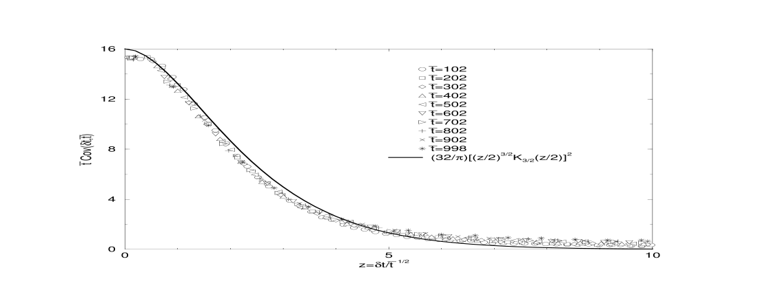
FIG. 11.: Plot of the intensity-covariance scaling function, $\bar{t}{\rm Cov}(\delta t,\bar{t}\,)$, versus $z=\delta t/\sqrt{\bar{t}}$ for different values of $\bar{t}$. The data collapse onto a single curve for a large range of $\bar{t}$. The solid curve is the corresponding analytic scaling function, $\bar{t}F^{2}_{2,{\rm YJ}}(\delta t,\bar{t}\,)$, predicted from the Yeung-Jasnow result in Eq. (38). It agrees quite well with the simulation data.

REFERENCES

- [1] M. Sutton, S. E. Nagler, S. G. Mochrie, T. Greytak, L. E. Bermann, G. Held, and G. B. Stephenson, Nature, 352, 608 (1991).
- [2] A comprehensive review is given by J. D. Gunton, M. San Miguel and P. S. Sahni, in Phase Transitions and Critical Phenomena, Vol. 8, edited by C. Domb and J. L. Lebowitz (Academic, London, 1983). Ideas of scaling in domain growth follow similar ideas in critical dynamics, P. C. Hohenberg and B. I. Halperin, Rev. Mod. Phys. 49, 435 (1977). A recent specialized review is given by A. J. Bray, Adv. Phys. 43, 357 (1994).
- [3] S. E. Nagler, R. F. Shannon, Jr., C. R. Harkless, and M. A. Singh, Phys. Rev. Lett. 61, 718 (1988); R. F. Shannon, Jr., S. E. Nagler, C. R. Harkless, and R. M. Nicklow, Phys. Rev. B 46, 40 (1992).
- [4] C. Roland and M. Grant, Phys. Rev. Lett. 63, 551 (1989).
- [5] B. Chu, Laser Light Scattering (Academic Press, New York, 1974).
- [6] L. Mandel and E. Wolf, Optical Coherence and Quantum Optics (Cambridge University Press, Cambridge, 1995).
- [7] S. B. Dierker, R. Pindak, R. M. Fleming, I. K. Robinson, and L. Berman, Phys. Rev. Lett. 75, 449 (1995).
- [8] B. Chu, Q.-C. Ying, F.-J. Yeh, A. Patkowski, W. Steffen, and E. W. Fischer, Langmuir 11, 1419 (1995).
- [9] S. Brauer, G. B. Stephenson, M. Sutton, R. Brüning, E. Dufresne, S. G. J. Mochrie, G. Grübel, J. Als-Nielsen, and D. L. Abernathy, Phys. Rev. Lett. 74, 2010 (1995).
- [10] S. G. J. Mochrie, A. M. Mayes, A. R. Sandy, M. Sutton, S. Brauer, G. B. Stephenson, D. L. Abernathy, and G. Grübel, Phys. Rev. Lett. 78, 1275 (1997).
- [11] E. Hernández-García and M. Grant, J. Phys. A 25, L1195 (1993).
- [12] E. Dufresne, Ph. D. thesis (McGill University, 1995); E. Dufresne, M. Sutton, K. Elder, B. Morin, M. Grant, B. Rodricks, G. B. Stephenson, G. B. Held, C. Thompson, S. G. J. Mochrie, S. E. Nagler, L. E. Berman, and R. Headrick (preprint, 1997).
- [13] J. Feder, Fractals (Plenum Press, New York, 1988).
- [14] A rough, quantitative measure of the different degrees of persistence can be obtained by application of Range/Scale (R/S) analysis [13] to the short sample time series shown in Fig. 3. This yields a Hurst exponent of approximately 0.54 for the “Brownian” function (near the expected value of 1/2), and a significantly larger value of approximately 0.74 for the normalized scattering intensity. However, the correlation times of these normalized time series are slowly increasing. Thus, the processes are not stationary, and the direct application of R/S analysis is only to be regarded as an approximate way of estimating the degree of persistence.
- [15] G. Brown, P. A. Rikvold, and M. Grant, Physica A 239, (1997).
- [16] Y. Oono and S. Puri, Phys. Rev. Lett. 58, 836 (1987).
- [17] H. Tomita, Prog. Theor. Phys. 85, 47 (1991).
- [18] T. Ohta, D. Jasnow, and K. Kawasaki, Phys. Rev. Lett. 49, 1223 (1982).
- [19] K. Kawasaki, M. C. Yalabik, and J. D. Gunton, Phys. Rev. A 17, 455 (1978).
- [20] It is natural to normalize the covariance by the standard deviations. In dynamic light-scattering, the autocorrelation function is normalized by the average intensity. For random Gaussian fluctuations, these are equal. See Eq. (27).
- [21] A. Milchev, K. Binder, and D. W. Heermann, Z. Phys. B 63, 521 (1986).
- [22] A. Shinozaki and Y. Oono, Phys. Rev. E 48, 2622 (1993).
- [23] N. B. Wilding, C. Münkel and D. W. Heerman, Z. Phys. B, 94, 301 (1994).
- [24] C. Yeung and D. Jasnow, Phys. Rev. B 42, 10523 (1990).
- [25] T. Ohta, Ann. Phys. (NY) 158, 31 (1984).
- [26] F. Liu and G. F. Mazenko, Phys. Rev. B 44, 9185 (1991).
- [27] G. F. Mazenko, Phys. Rev. B 42, 4487 (1990).
- [28] C. Yeung, M. Rao and R. C. Desai, Phys. Rev. E 53, 3073 (1996).
- [29] D. S. Fisher and D. A. Huse, Phys. Rev. B 38, 373 (1988). See also, S. N. Majumdar, D. A. Huse, and B. D. Lubachevsky, Phys. Rev. Lett. 73, 182 (1994).
- [30] N. Mason, A. N. Pargellis, and B. Yurke, Phys. Rev. Lett. 70, 190 (1993).