Spectral Function of 2D Fermi Liquids

Abstract

We show that the spectral function for single-particle excitations in a two-dimensional Fermi liquid has Lorentzian shape in the low energy limit. Landau quasi-particles have a uniquely defined spectral weight and a decay rate which is much smaller than the quasi-particle energy. By contrast, perturbation theory and the T-matrix approximation yield spurious deviations from Fermi liquid behavior, which are particularly pronounced for a linearized dispersion relation.

1. Introduction

The low energy physics of interacting Fermi systems is usually governed by Landau’s Fermi liquid theory, as long as no binding or symmetry-breaking occurs [1]. Fermi liquid theory is based on the existence of quasi-particles, i.e. fermionic single-particle excitations with an energy-momentum relation $\xi_{{\bf k}}$ that vanishes linearly as ${\bf k}$ approaches the Fermi surface $\cal F$ of the system. In three-dimensional Fermi liquids quasi-particles decay with a rate $\gamma_{{\bf k}}$ that vanishes quadratically near $\cal F$, as a consequence of the restricted phase space for low-energy scattering processes. The single-particle spectral function $\rho({\bf k},\xi)$ exhibits a Lorentzian-shaped peak of width $\gamma_{{\bf k}}$ as a function of the energy variable $\xi$ for ${\bf k}$ close to $\cal F$.

In one-dimensional Fermi systems Landau’s quasi-particles are unstable: the decay rate of single-particle excitations with sharp momenta is at least of the order of their energy and their spectral weight vanishes in the low-energy limit, giving rise to so-called Luttinger liquid behavior [2].

No consensus has so far been reached on the properties of single-particle excitations in two-dimensional Fermi systems. The anomalous properties of electrons moving in the $\mathrm{CuO_{2}}$-planes of high-$T_{c}$ superconductors have motivated numerous speculations on a possible breakdown of Fermi liquid theory in 2D systems, at least for sufficiently strong interaction strength [3] and, according to Anderson [4], even for weak coupling.

The development of new powerful renormalization group techniques [5, 6] has recently opened the way towards a rigorous non-perturbative control of interacting Fermi systems for sufficiently small yet finite coupling strength [7]. Significant rigorous results have already been derived for 2D systems. For example, the existence of a finite jump in the momentum distribution has been established for two-dimensional Fermi systems with a non-symmetry-broken ground state [8]. This excludes Luttinger liquid behavior in weakly interacting 2D systems.

So far, however, no rigorous results could be obtained for real-time (or frequency) dynamic quantities such as spectral functions. In particular, even at weak coupling the shape of the spectral function for single-particle excitations and the existence of well-defined quasi-particles are still under debate. Indeed, within second order perturbation theory the imaginary part of the self-energy $\Sigma({\bf k},\xi)$ exhibits a sharp peak near $\xi=\xi_{{\bf k}}$ in two dimensions [9], to be contrasted with the simple quadratic and ${\bf k}$-independent energy-dependence of ${\rm Im}\Sigma({\bf k},\xi)$ in 3D. Such a peak in the self-energy leads to a spectral function with two separate maxima instead of a single quasi-particle peak [9, 10]. However, analyzing an analytic continuation of one-dimensional Luttinger liquids to higher dimensionality $d$, Castellani, Di Castro and one of us [9, 3] have pointed out that such peaks in the perturbative self-energy are smeared out in a random phase approximation (RPA) and probably also in an exact solution. Most recently a breakdown of Fermi liquid theory has been inferred from a divergence of the slope of the self-energy, computed within a T-matrix approximation (TMA), at $\xi=\xi_{{\bf k}}$ [11].

In this article we present explicit results for the self-energy computed within perturbation theory, TMA and RPA for a two-dimensional prototypical model with local interactions. We will then provide several simple arguments showing that the RPA, which yields a Fermi liquid type result for self-energy and spectral function, is qualitatively correct, while unrenormalized perturbation theory and the T-matrix approximation produce artificial singularities in 2D systems.

2. Perturbation theory and T-matrix

We consider an isotropic continuum model with a local coupling as a prototype for Fermi systems with short-range repulsive interactions,

$$H=\sum_{{\bf k},\sigma}\epsilon_{{\bf k}}\,a^{{\dagger}}_{{\bf k}\sigma}a_{{\bf k}\sigma}\,+\,{g\over V}\sum_{{\bf k},{\bf k}^{\prime},{\bf q}}a^{{\dagger}}_{{\bf k}+{\bf q}\uparrow}a_{{\bf k}\uparrow}\>a^{{\dagger}}_{{\bf k}^{\prime}-{\bf q}\downarrow}a_{{\bf k}^{\prime}\downarrow},$$ (1)

where $a^{{\dagger}}_{{\bf k}\sigma}$ and $a_{{\bf k}\sigma}$ are the usual creation and annihilation operators for spin-$1\over 2$ fermions, $\epsilon_{{\bf k}}$ is an (isotropic) dispersion relation, $g\!>\!0$ a coupling constant, and $V$ the volume of the system. Local interactions between particles with parallel spin do not contribute due to the Pauli exclusion principle. A cutoff must be imposed for large momenta to make the model well-defined.

The spectral function for single-particle excitations $\rho({\bf k},\xi)$ is directly related to the imaginary part of the one-particle Green function at real frequencies [12]

$$G({\bf k},\xi)={1\over\xi-(\epsilon_{{\bf k}}-\mu)-\Sigma({\bf k},\xi)}.$$ (2)

Here $\mu$ is the chemical potential (fixing the particle density). Note that $\rho({\bf k},\xi)$ can be measured by angular resolved photoemission.

To first order in the coupling constant $g$, the self-energy is a constant which can be absorbed by shifting the chemical potential. Non-trivial dynamics enters at second order, where for a local interaction only a single Feynman diagram (see Fig. 1)

Figure 1: Second order Feynman diagram contributing to $\Sigma({\bf k},\xi)$.

yields an energy-dependent contribution $\Sigma^{(2)}({\bf k},\xi)$. The imaginary part, ${\rm Im}\Sigma^{(2)}({\bf k},\xi)$, is cutoff independent and can be expressed as a two-dimensional integral, which can be easily performed numerically. Low-energy results for a quadratic (free-particle) dispersion $\epsilon_{{\bf k}}={\bf k}^{2}/2m$ and a linear dispersion $\epsilon_{{\bf k}}=v_{F}|{\bf k}|$ are shown in Fig. 2.

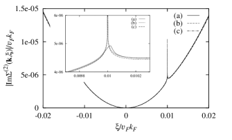
Figure 2: Numerical results for ${\rm Im}\Sigma^{(2)}({\bf k},\xi)$ at fixed $|{\bf k}|=1.01k_{F}$ for (a) a quadratic and (b) a linear dispersion relation, compared to (c) the asymptotic analytic result (3). The fine-structure of the peak near $\xi=\xi_{{\bf k}}$ is shown in the inset.

The Fermi momentum $k_{F}$ and the Fermi velocity $v_{F}$ has been set one in both cases ($v_{F}=k_{F}/m$ for quadratic dispersion), and ${\bf k}$ has been fixed slightly outside the Fermi surface, i.e. $|{\bf k}|=1.01k_{F}$. Note that the two curves almost coincide except very close to the point $\xi=\xi_{{\bf k}}=\epsilon_{{\bf k}}\!-\!\mu$, while the structure of the peak near $\xi_{{\bf k}}$ depends sensitively on the curvature of $\epsilon_{{\bf k}}$ near $k_{F}$. Indeed, a strikingly simple analytic expression can be derived for the asymptotic low-energy behavior of ${\rm Im}\Sigma^{(2)}$ (see Appendix):

$$\begin{array}[]{l}\displaystyle|{\rm Im}\Sigma^{(2)}({\bf k},\xi)|=g^{2}\,{k_{F}\over(2\pi)^{3}v_{F}^{3}}\,\xi^{2}\times\\ \displaystyle\qquad\times\left[1+\ln 4\sqrt{3}-{3\over 2}\ln|\xi/v_{F}k_{F}|-{\kappa\over 2}-\ln|\kappa+1|\right.\\ \displaystyle\qquad\left.-{1\over 2}\ln|\kappa-1|+{1\over 4}(\kappa-1)^{2}\ln\left|{\kappa+1\over\kappa-1}\right|\right]\,+\,{\cal O}(|\xi|^{5/2})\\ \end{array}$$ (3)

for small $\xi$ at fixed $\kappa=\xi_{{\bf k}}/\xi\neq 1$. For generic (non-linear) dispersion relations there are non-universal deviations from the leading asymptotic result in a tiny region of width $\xi_{{\bf k}}^{2}$ around $\xi=\xi_{{\bf k}}$. For ${\bf k}={\bf k}_{F}$ (i.e. $\kappa=0$) one recovers the known perturbative result ${\rm Im}\Sigma^{(2)}({\bf k}_{F},\xi)\propto\xi^{2}\log|\xi|+{\cal O}(|\xi|^{2})$ [13]. The logarithmic singularity for $\xi\sim\xi_{{\bf k}}$ has already been noted earlier in the literature [9, 10], but the complete asymptotic low-energy expression (3) for the second order self-energy has not been found so far.

As pointed out in another context by Castellani et al. [9] and also by Fukuyama and Ogata [10], a peak in the self-energy as in Fig. 2 would lead to a spectral function with two maxima centered around the quasi-particle energy $\xi_{{\bf k}}$, which is reminiscent of the two-peak structure of spectral functions in one-dimensional Luttinger liquids [14, 2].

Several authors have computed the self-energy for two-dimensional Fermi systems within the so-called T-matrix approximation (TMA), i.e. summing all particle-particle ladder diagrams [15, 16, 17]. This approximation is expected to be asymptotically exact at low density $n\to 0$ in dimensions $d\geq 2$, where corrections are smaller by a factor $n$ in 3D but only by a factor $1/|\log(n)|$ in 2D [17]. Numerical results for the imaginary part of the T-matrix self-energy $\Sigma^{T}({\bf k},\xi)$, calculated for the model (1), are shown in Fig. 3.

Figure 3: Numerical results for ${\rm Im}\Sigma({\bf k},\xi)$ at fixed $|{\bf k}|=1.001k_{F}$ within second order perturbation theory, TMA and RPA, for a coupling $g=1{v_{F}\over k_{F}}$ and a quadratic $\epsilon_{{\bf k}}$; the TMA requires a cutoff for large momenta which has been chosen as $\Lambda=5k_{F}$.

The peak at $\xi\!=\!\xi_{{\bf k}}$ is now bounded even for a linear $\epsilon_{{\bf k}}$. However, Yokoyama and Fukuyama [11] have recently found that the real part of $\Sigma^{T}({\bf k},\xi)$ has infinite slope at $\xi=\xi_{{\bf k}}$ for a linearized dispersion relation. Evaluating the renormalization factor

$$Z({\bf k},\xi)=\left[1-\partial\Sigma({\bf k},\xi)/\partial\xi\right]^{-1}$$ (4)

in the special limit ${\bf k}\to{\bf k}_{F}$, $\xi\to 0$ with $\xi/\xi_{{\bf k}}\to 1$ they obtained the result ”$Z\to 0$”, which was interpreted as a confirmation of Anderson’s [4] ideas about a breakdown of Fermi liquid theory in two dimensions. This interpretation seems to be misleading. Firstly, one cannot replace the function $Z({\bf k},\xi)$ by a single number ”$Z$” if $Z({\bf k},\xi)$ has no (unique) limit for ${\bf k}\to{\bf k}_{F}$, $\xi\to 0$. Indeed, $Z({\bf k},\xi)$ vanishes only in the above special limit. In particular, the jump in the momentum distribution function across the Fermi surface, which is also given by ”$Z$” in a conventional Fermi liquid, does not vanish within the TMA in 2D systems! Secondly, one cannot trust a singular result for a correlation function obtained from a truncated asymptotic expansion with respect to a ”small” parameter, since higher order corrections are generally not uniformly small for all momenta and energies. One should be even more worried in a case where corrections are suppressed at best by logarithmic factors $1/|\log(n)|$ [18]. Indeed, the artificial sensitivity of the peaks in $\Sigma({\bf k},\xi)$ on irrelevant non-linear terms in the dispersion relation found in perturbation theory and TMA indicates that the exact self-energy will look differently.

3. Random phase approximation

A self-energy with a regular energy-dependence which does not depend sensitively on irrelevant terms in $\epsilon_{{\bf k}}$ is obtained from the random phase approximation

$$\Sigma^{RPA}({\bf k},\xi)=i\int{d^{2}q\over(2\pi)^{2}}\int{d\omega\over 2\pi}\,D({\bf q},\omega)\,G^{(0)}({\bf k}\!-\!{\bf q},\xi\!-\!\omega),$$ (5)

where $G^{(0)}$ is the non-interacting Green function and $D$ the RPA effective interaction between particles with parallel spin projection. For the locally interacting model, (1),

$$D({\bf q},\omega)={g^{2}\Pi^{(0)}({\bf q},\omega)\over 1-g^{2}\left[\Pi^{(0)}({\bf q},\omega)\right]^{2}},$$ (6)

where $\Pi^{(0)}$ is the non-interacting polarization function. Numerical results for ${\rm Im}\Sigma^{RPA}$ are shown in Fig. 3. In contrast to the single sharp peak near $\xi=\xi_{{\bf k}}$ obtained in perturbation theory and TMA, the RPA result exhibits two smooth maxima with a width that is of the same order of magnitude as their height. These maxima are due to long-wavelength collective charge and spin density fluctuations which contribute significantly to the RPA effective interaction; such collective fluctuations are not described by perturbation theory or TMA. The corresponding spectral function has Lorentzian shape, with a smooth background that vanishes quickly in the low energy limit. The quasi-particle decay rate $\gamma_{{\bf k}}$ can thus be computed unambiguously from ${\rm Im}\Sigma^{RPA}({\bf k},\xi_{{\bf k}})$ and turns out to be proportional to $(k\!-\!k_{F})^{2}\log|k\!-\!k_{F}|$ for arbitrary $\epsilon_{{\bf k}}$ (while the perturbative ${\rm Im}\Sigma^{(2)}({\bf k},\xi_{\bf k})$ is infinite for a linear $\epsilon_{{\bf k}}$, and finite else). The renormalization function $Z({\bf k},\xi)$ computed from the RPA self-energy has a unique limit $Z$ for ${\bf k}\to{\bf k}_{F}$, $\xi\to 0$.

The peaks in $\Sigma({\bf k},\xi)$ near $\xi=\xi_{{\bf k}}$ are produced by virtual excitations where the excited particles and holes have low energies and momenta near the Fermi surface close to the quasi-particle momentum ${\bf k}$. In 3D systems the phase space for these particular excitations is very small and the low-energy behavior of ${\rm Im}\Sigma$ is dominated by low-energy particle-hole excitations with momenta all over the Fermi surface. Second order perturbation theory, TMA and RPA all yield the same simple behavior ${\rm Im}\Sigma({\bf k},\xi)\propto\xi^{2}$ with a possible weak ${\bf k}$-dependence in the prefactor. In fact a renormalized perturbation theory where the bare interaction is replaced by the exact quasi-particle scattering amplitudes yields the exact leading low-energy terms of ${\rm Im}\Sigma$ in 3D already at second order (in the scattering amplitudes) [19]. For dimensionality $d\leq 2$ this is not true because virtual excitations with small momentum transfers dominate ${\rm Im}\Sigma$ [3]. Their contribution depends on the strength of the interaction vertex for small momentum transfers ${\bf q}$ (i.e. in the forward scattering channel) which is itself strongly renormalized by low-energy excitations [3]! Since the polarization function $\Pi^{(0)}({\bf q},\omega)$ has contributions exclusively from low-energy states for small ${\bf q}$, it is reasonable to reorganize the perturbation series by replacing bare interactions with RPA effective interactions. The simplest approximation for the self-energy is then to dress the bare fermionic propagator by only one effective interaction. It has been pointed out already earlier by Eschrig et al. [20] that all RPA diagrams yield equally important contributions to $\Sigma$ in a renormalized low-energy expansion in two dimensions.

The random phase approximation is not an arbitrary resummation of Feynman diagrams, but is controlled by the expansion parameter $1/N$, where $N$ is the number of spin states in a generalization of model (1), where instead of two possible spin-projections one allows for $N$ different spin states. Rescaling the coupling constant by a factor $1/N$, one can take the large $N$ limit and classify Feynman diagrams by powers of $1/N$. Since each interaction line in a diagram yields a factor $1/N$ and each closed loop a factor $N$, all non-RPA contributions are of order $(1/N)^{2}$. In contrast to plain perturbation theory and the TMA, which are controlled by the coupling constant $g$ and factors $1/|\log(n)|$, respectively, the RPA yields a regular result for $\Sigma({\bf k},\xi)$. Thus $1/N$ seems to be a suitable expansion parameter for 2D Fermi liquids, with higher order corrections being uniformly small for all ${\bf k}$, $\xi$ (for large $N$).

Even more convincing is a comparison with one-dimensional Fermi systems, where exact results are available [2]. Since the peaks in the self-energy discussed above are due to excitations of particles and holes with almost equal momenta, it is sufficient to consider a special case of the exactly soluble Luttinger model where only the particles and holes near the right (or left) Fermi point interact. In Fig. 4

Figure 4: ${\rm Im}\Sigma(k,\xi)$ at fixed $k=1.001k_{F}$ for a one-dimensional model with a linear dispersion relation and a coupling $g=1v_{F}$; the exact result is compared to perturbation theory and RPA (the vertical arrow represents a $\delta$-function).

we show the exact result for ${\rm Im}\Sigma(k,\xi)$ for this model, compared to the RPA result and the result of second order perturbation theory. The sharp peak (a $\delta$-function for a linearized dispersion) appearing in perturbation theory is replaced by a smooth maximum with equal height and width in the exact solution. The RPA correctly captures the width and height of the exact function, though not its form. One may thus guess that the two broad maxima in ${\rm Im}\Sigma({\bf k},\xi)$ obtained from the RPA in 2D have to be replaced by one broad maximum in the full solution. In any case the spectral function will have Lorentzian shape. Note that the RPA correctly signals all the non-Fermi liquid singularities in one dimension (${\rm Im}\Sigma^{RPA}(k,\xi)$ is linear in $k\!-\!k_{F}$, $\xi$ in 1D), while it yields regular Fermi liquid behavior in 2D.

Our explicit (numerical and analytical) results have been obtained for an isotropic model with a weak local interaction. The qualitative conclusions hold more generally for any Fermi liquid with short-range interactions and a Fermi surface with finite curvature, as long as no instability associated with diverging renomalized interactions occurs.

4. Conclusion

In summary, we have shown that the spectral function for single-particle excitations in a two-dimensional Fermi liquid with short-range interactions has Lorentzian shape. Quasi-particles have a uniquely defined spectral weight $Z$ (equal to the jump of the momentum distribution across the Fermi surface) and a decay rate proportional to $k^{\prime 2}\log k^{\prime}$, where $k^{\prime}$ is the distance of the quasi-particle momentum from the Fermi surface. The latter result is not new, but is has so far been derived only by ”good luck”, i.e. by computing ${\rm Im}\Sigma({\bf k},\xi_{{\bf k}})$ within perturbation theory [21] or TMA [15] for a quadratic dispersion, where the spurious peak in ${\rm Im}\Sigma({\bf k},\xi)$ reaches its maximum at an energy of order $\xi_{{\bf k}}^{2}/\epsilon_{F}$ below $\xi_{{\bf k}}$! We have provided several arguments showing that the random phase approximation yields a qualitatively correct result for the spectral function, while plain perturbation theory and the T-matrix approximation produce spurious singularities.

Acknowledgements: We are grateful to H. Knörrer, E. Müller-Hartmann, M. Salmhofer, and E. Trubowitz for valuable discussions. This work has been supported by the Deutsche Forschungsgemeinschaft under contract no. Me 1255/4-1.

Appendix:
Self-energy in second order perturbation theory

For the continuum model (1) the second order contribution to the (time-ordered) self-energy can be calculated using the two-particle propagator $K({\bf p},\omega)=i\int\frac{d^{2}k}{(2\pi)^{2}}\int\frac{d\xi}{2\pi}\,G^{(0)}({\bf p}-{\bf k},\omega-\xi)\,G^{(0)}({\bf k},\xi)$. In the following we make use of the spectral representations of the self-energy, $\Sigma({\bf k},\xi)=\int d\xi^{\prime}\,S({\bf k},\xi^{\prime})/(\xi-\xi^{\prime}+i0^{+}{\rm sgn\>}\xi^{\prime})$, the free one-particle propagator, $G^{(0)}({\bf k},\xi)=\int d\xi^{\prime}\,\rho^{(0)}({\bf k},\xi^{\prime})/(\xi-\xi^{\prime}+i0^{+}{\rm sgn\>}\xi^{\prime})$, and the two-particle propagator, $K({\bf p},\omega)=\int d\omega^{\prime}\,\Delta^{pp}({\bf p},\omega^{\prime})/(\omega-\omega^{\prime}+i0^{+}{\rm sgn\>}\omega^{\prime})$. For a quadratic dispersion $\epsilon_{{\bf k}}={\bf k}^{2}/2m$, $\Delta^{pp}$ is given by [16]

$$\Delta^{pp}(p,\omega)=\left\{\begin{array}[]{lll}0&\!\!\mbox{if}&\!\!\omega<\omega_{0}\\ \frac{N_{F}}{2}{\rm sgn\>}\omega&\!\!\mbox{if}&\!\!\omega_{0}<\omega<\omega_{-}\\ \frac{N_{F}}{\pi}\arcsin\left(\frac{\omega}{p}\frac{1}{\sqrt{\omega-\omega_{0}}}\right)&\!\!\mbox{if}&\!\!\omega_{-}<\omega<\omega_{+}\\ \frac{N_{F}}{2}&\!\!\mbox{if}&\!\!\omega_{+}<\omega,\end{array}\right.$$ (A.1)

where $\omega_{0}:=p^{2}/4-1$, $\omega_{\pm}:=p^{2}/2\pm p$, and the free density of states $N_{F}=k_{F}/2\pi v_{F}$. Here and in the following momentum variables are measured in units of $k_{F}$ and energy variables in units of $v_{F}k_{F}$.

The second order contribution to the spectral function of the self-energy can be written as

$$\begin{array}[]{l}\displaystyle S({\bf k},\xi)=g^{2}\int_{0}^{\xi}\!\frac{d\omega}{2\pi}\int\!\frac{d^{2}p}{(2\pi)^{2}}\Delta^{pp}({\bf p},\omega)\,\rho^{(0)}({\bf p}\!-\!{\bf k},\omega\!-\!\xi)\\ \displaystyle\quad=\frac{g^{2}N_{F}}{2\pi}v_{F}k_{F}\int_{0}^{\xi}\!d\omega\int_{0}^{\infty}\!dp\,p\,\Delta^{pp}(p,\omega)\bar{\rho}(k,p;\omega-\xi).\end{array}$$ (A.2)

Here

$$\begin{array}[]{l}\displaystyle\bar{\rho}(k,p;\zeta):=2\int_{0}^{\pi}d\phi\,\delta(\zeta-\xi_{{\bf p}-{\bf k}})\\ \displaystyle\quad=4\frac{\Theta\left((p^{2}-(k-\sqrt{2\zeta+1})^{2})((k+\sqrt{2\zeta+1})^{2}-p^{2})\right)}{\sqrt{(p^{2}-(k-\sqrt{2\zeta+1})^{2})((k+\sqrt{2\zeta+1})^{2}-p^{2})}}\end{array}$$ (A.3)

is the angle-integrated imaginary part of the free propagator $G^{(0)}$, $\phi$ being the angle between ${\bf p}$ and ${\bf k}$ [16].

For small $\xi\ll 1$ the integration boundaries $|k-\sqrt{2\zeta+1}|<p<k+\sqrt{2\zeta+1}$, given by the step-function $\Theta$ in eq. (A.3), can be linearized to $|k-\zeta-1|<p<k+\zeta+1$. The same can be done with the boundaries $\omega_{0}$, $\omega_{\pm}$ in eq. (A.1). This leaves us with trapezoid integration regions as given by the shaded areas in Fig. 5 for the case $\xi\geq 0$ and $k-k_{F}\geq 0$.

Figure 5: Integration boundaries in the $(p,\omega)$ plane for $0\leq\xi\ll 1$ and $\epsilon:=k-k_{F}\geq 0$. $p$, $\epsilon$ in units of $k_{F}$; $\omega$, $\xi$ in units of $v_{F}k_{F}$.

Also shown in Fig. 5 are subareas $(1)$ – $(3)$, which can be defined analogously for other choices of $\xi$ and $k$. In these subareas we can use the following asymptotic expressions for $\bar{\rho}$ and $\Delta^{pp}$ ($\epsilon:=k-k_{F}$):

$$\bar{\rho}(k,p,\zeta)\approx\left\{\!\begin{array}[]{lll}\frac{2}{\sqrt{p^{2}-(\epsilon-\zeta)^{2}}}&\!\mbox{if}&\!(p,\zeta)\in(1),(1a),1(b)\\ \frac{4}{p\sqrt{(2+\epsilon+\zeta)^{2}-p^{2}}}&\!\mbox{if}&\!(p,\zeta)\in(2)\\ \frac{2}{\sqrt{(2+\epsilon+z)^{2}-p^{2}}}&\!\mbox{if}&\!(p,\zeta)\in(3),\end{array}\right.$$ (A.4)

$$\Delta^{pp}(p,\omega)\approx\left\{\!\!\begin{array}[]{lll}\frac{N_{F}}{2}{\rm sgn\>}\omega&\!\!\!\!\mbox{if}&\!\!\!\!(p,\zeta)\in(1a)\\ \frac{N_{F}}{\pi}\arcsin\frac{\omega}{p}&\!\!\!\!\mbox{if}&\!\!\!\!(p,\zeta)\in(1),(1b)\\ \frac{N_{F}}{\pi}\frac{2\omega}{p\sqrt{(2+\omega)^{2}-p^{2}}}&\!\!\!\!\mbox{if}&\!\!\!\!(p,\zeta)\in(2)\\ \frac{N_{F}}{\pi}\arctan\frac{\omega}{\sqrt{(2+\omega)^{2}-p^{2}}}&\!\!\!\!\mbox{if}&\!\!\!\!(p,\zeta)\in(3).\end{array}\right.$$ (A.5)

These approximations lead to a result for the self-energy which is exact within second order in $\xi$ at fixed $\kappa:=\xi_{\bf k}/\xi\neq 1$.

With these asymptotic expressions the integration over $p$ can be performed analytically. The results for the different subareas are rather lengthy, but can be simplified by a further expansion in $\omega=\cal{O}(\xi)$ and $\epsilon=\cal{O}(\xi)$, keeping the ratio $\kappa=\epsilon/\omega$ fixed. Now also the integration over $\omega$ can be performed analytically, resulting in the simple expression eq. (3) (Note that $S({\bf k},\xi)=|{\rm Im}\Sigma({\bf k},\xi)|/\pi$). The main contributions to $S$ come from the momenta $p\approx 0$ and $p\approx 2k_{F}$. The contributions from $p\approx 0$ are

$$\begin{array}[]{l}\displaystyle S_{p\approx 0}({\bf k},\xi)=g^{2}\frac{N_{F}^{2}v_{F}k_{F}}{2\pi^{2}}\xi^{2}\left[1+\ln 2-\ln|\xi|-\frac{1}{2}\kappa-\phantom{\frac{1}{2}}\right.\\ \displaystyle\qquad\qquad\qquad\left.-\ln\left|\kappa+1\right|+\frac{1}{4}\left(\kappa-1\right)^{2}\ln\left|\frac{\kappa+1}{\kappa-1}\right|\right].\end{array}$$ (A.6)

The contributions from $p\approx 2k_{F}$ are

$$\begin{array}[]{l}\displaystyle S_{p\approx 2k_{F}}({\bf k},\xi)=g^{2}\frac{N_{F}^{2}v_{F}k_{F}}{2\pi^{2}}\xi^{2}\times\\ \displaystyle\qquad\qquad\qquad\,\times\left[\ln 2\sqrt{3}-\frac{1}{2}\ln|\xi|-\frac{1}{2}\ln\left|\kappa-1\right|\right],\end{array}$$ (A.7)

causing the logarithmic divergence at $\kappa=1$.

References

- [1] L.D. Landau, Sov. Phys. JETP 3, 920 (1956); ibid 5, 101 (1957).
- [2] For a comprehensive up-to-date review on one-dimensional Fermi systems, see J. Voit, Rep. Prog. Phys. 58, 977 (1995).
- [3] For a review on Fermi systems with strong forward scattering, see W. Metzner, C. Castellani and C. Di Castro, cond-mat/9702012, Adv. Phys. (in press).
- [4] P. W. Anderson, Phys. Rev. Lett. 64, 1839 (1990); Phys. Rev. Lett. 65, 2306 (1990).
- [5] J. Feldman and E. Trubowitz, Helv. Phys. Act. 63, 156 (1990); 64, 213 (1991); 65, 679 (1992).
- [6] G. Benfatto and G. Gallavotti, Phys. Rev. B42, 9967 (1990); J. Stat. Phys. 59, 541 (1990).
- [7] J. Feldman, J. Magnen, V. Rivasseau, and E. Trubowitz in The State of Matter, M. Aizenmann and H. Araki eds, Advanced Series in Mathematical Physics Vol. 20 (World Scientific, 1994).
- [8] J. Feldman, H. Knörrer, D. Lehmann and E. Trubowitz in Constructive Physics, ed. V. Rivasseau, Springer Lecture Notes in Physics (Springer 1995); J. Feldman, M. Salmhofer and E. Trubowitz, J. Stat. Phys. 84, 1209 (1996); preprint mp-arc 96-684; preprint mp-arc 97-287.
- [9] C. Castellani, C. Di Castro and W. Metzner, Phys. Rev. Lett. 72, 316 (1994).
- [10] H. Fukuyama and M. Ogata, J. Phys. Soc. Jpn. 63, 3923 (1995).
- [11] K. Yokoyama and H. Fukuyama, J. Phys. Soc. Jpn. 66, 529 (1997).
- [12] A.A. Abrikosov, L.P. Gorkov, and I.E. Dzyaloshinski, Methods of Quantum Field Theory in Statistical Physics (Dover, New York 1975).
- [13] S. Fujimoto, J. Phys. Soc. Jpn. 59, 2316 (1990).
- [14] V. Meden and K. Schönhammer, Phys. Rev. B 46, 15753 (1992); J. Voit, Phys. Rev. B 47, 6740 (1993).
- [15] P. Bloom, Phys. Rev. B 12, 125 (1975).
- [16] H. Fukuyama, Y. Hasegawa, and O. Narikiyo, J. Phys. Soc. Jpn. 60, 2013 (1991).
- [17] J.R. Engelbrecht and M. Randeria, Phys. Rev. B 45, 12419 (1992).
- [18] We would like to thank E. Müller-Hartmann for drawing our attention to this problem.
- [19] See for example, J.W. Serene and D. Rainer, Phys. Rep. 101, 221 (1983).
- [20] M. Eschrig, J. Heym, and D. Rainer, J. Low Temp. Phys. 95, 323 (1994).
- [21] C. Hodges, H. Smith, and J.W. Wilkins, Phys. Rev. B 4, 302 (1971).