INTERFACE PINNING

AND FINITE SIZE EFFECTS

IN THE 2D ISING MODEL

C.-E. Pfister, Y. Velenik

Département de Mathématiques, EPF-L

CH-1015 Lausanne, Switzerland

e-mail: charles.pfister@dma.epfl.ch

Département de Physique, EPF-L

CH-1015 Lausanne, Switzerland

e-mail: velenik@dpmail.epfl.ch

8 March 2024

Abstract: We apply new techniques developed in [PV1] to the study of some surface effects in the 2D Ising model. We examine in particular the pinning-depinning transition. The results are valid for all subcritical temperatures. By duality we obtained new finite size effects on the asymptotic behaviour of the two–point correlation function above the critical temperature. The key–point of the analysis is to obtain good concentration properties of the measure defined on the random lines giving the high–temperature representation of the two–point correlation function, as a consequence of the sharp triangle inequality: let $\hat{\tau}(x)$ be the surface tension of an interface perpendicular to $x$; then for any $x$, $y$

$$\hat{\tau}(x)+\hat{\tau}(y)-\hat{\tau}(x+y)\geq{1\over\kappa}\left(\|x\|+\|y\|-\|x+y\|\right)\,,$$

where $\kappa$ is the maximum curvature of the Wulff shape and $\|x\|$ the Euclidean norm of $x$.

Key Words: Ising model, pinning transition, reentrance, interface, surface tension, positive stiffness, correlation length, two–point function, finite size effects, concentration of measures.

1 Introduction

Consider a 2D Ising model in some rectangular box with boundary conditions implying the presence of a phase separation line crossing the box from one vertical side to the other one. The bottom side of the box, which we call the wall, is subject to a magnetic field $h$. By varying $\beta$ and/or $h$, when we are in the phase coexistence region, we can observe the so-called pinning–depinning transition, which occurs when the $+$ phase, which is above the interface, begins to wet the wall with the result that the equilibrium shape of the interface changes from a straight line crossing the box to a broken line touching a macroscopic part of the wall. This phenomenon has been recently studied by Patrick [Pa] in the SOS model using exact calculations. In the 2D Ising model this phenomenon has a dual interpretation at high temperature in terms of finite size effects on the asymptotic behaviour of two–point function for large distances. These questions can be analyzed in the 2D Ising model by the new non–perturbative results developed in [Pf2] and [PV1] in the context of large deviations and separation of phases. Some parts of the paper , like section 4, are written directly for the two–point function. Pinning–depinning transition and the finite size effects on the two–point correlation function are treated in section 6.

The fundamental thermodynamical function associated with an interface is the surface tension. The interface between the two phases of the model is a non–random object. On the other hand, at the scale of the lattice spacing, we have the random line, which is a geometrical object separating the two phases. The interface is therefore defined at a scale where the fluctuations of the phase separation line become negligible. Its main properties are described by a functional of the surface tension. The observed interface at equilibrium is a minimum of this functional (section 3). The study of fluctuations of the phase separation line is an important and difficult problem; some works in that directions are [Hi], [BLP1], [DH].

A key–point of the present analysis is the role of the sharp triangle inequality of the surface tension [I], which, combined with our recent results, leads to good concentration properties for the measure defined on the random lines giving the high–temperature representation of the two–point correlation function (section 4). (These random lines coincide with the phase–separation lines.) Because of its importance, we devote section 7 to a geometrical study of the sharp triangle inequality. This section can be read independently; Proposition 7.1 has its own interest.

The paper is not self–contained, because we use in an essential way results of [PV1], in particular those of section 5. They are carefully stated in Propositions 2.3 and 4.2 and Lemmas 5.1 and 5.2. This has the advantage that we can focus our attention on the essential points of the proofs. Motivated by [Pa] we have chosen pinning–depinning transition to illustrate the technique of [PV1]; we can consider more complicated situations than the ones of this paper.

Acknowledgments: We thank M. Troyanov for very useful discussions and suggestions about the geometrical aspect of section 7.

2 Definitions and notations

2.1 Phase separation line

We follow [PV1] for the notation and terminology. Throughout the paper $O(x)$ denotes a non–negative function of $x\in{{\rm I\!R}}^{+}$, such that there exists a constant $C$ with $O(x)\leq Cx$. The function $O(x)$ may be different at different places.

Let $Q$ be the square box in ${{\rm I\!R}}^{2}$,

$$Q:=\{\,x=(x(1),x(2))\in{{\rm I\!R}}^{2}:\,|x(1)|\leq 1/2\;,\;0\leq x(2)\leq 1\,\}\,,$$ (2.1)

and $\Lambda_{L}$ be the subset of ${{\mathchoice{\hbox{$\sf\textstyle Z\kern-3.99994ptZ$}}{\hbox{$\sf\textstyle Z\kern-3.99994ptZ$}}{\hbox{$\sf\scriptstyle Z\kern-2.10002ptZ$}}{\hbox{$\sf\scriptscriptstyle Z\kern-0.99998ptZ$}}}}^{2}$ ($L$ an even integer)

$$\Lambda_{L}:=\{\,x=(x(1),x(2))\in{{\mathchoice{\hbox{$\sf\textstyle Z\kern-3.99994ptZ$}}{\hbox{$\sf\textstyle Z\kern-3.99994ptZ$}}{\hbox{$\sf\scriptstyle Z\kern-2.10002ptZ$}}{\hbox{$\sf\scriptscriptstyle Z\kern-0.99998ptZ$}}}}^{2}:\,|x(1)|\leq L/2\;,\;0\leq x(2)\leq L\,\}\,.$$ (2.2)

The spin variable at $x\in{{\mathchoice{\hbox{$\sf\textstyle Z\kern-3.99994ptZ$}}{\hbox{$\sf\textstyle Z\kern-3.99994ptZ$}}{\hbox{$\sf\scriptstyle Z\kern-2.10002ptZ$}}{\hbox{$\sf\scriptscriptstyle Z\kern-0.99998ptZ$}}}}^{2}$ is the random variable $\sigma(x)=\pm 1$; spin configurations are denoted by $\omega\in\{-1,+1\}^{{{\mathchoice{\hbox{$\sf\textstyle Z\kern-2.79996ptZ$}}{\hbox{$\sf\textstyle Z\kern-2.79996ptZ$}}{\hbox{$\sf\scriptstyle Z\kern-1.47002ptZ$}}{\hbox{$\sf\scriptscriptstyle Z\kern-0.69998ptZ$}}}}^{2}}$, so that $\sigma(t)(\omega)=\pm 1$ if $\omega(t)=\pm 1$. We always suppose that we have for the box $\Lambda_{L}$ either the $ab$ boundary condition ($ab$ b.c.) or the $-$ boundary condition ($-$ b.c.). Let $0\leq a\leq 1$ and $0\leq b\leq 1$ be given; the $ab$ b.c. specifies the values of the spins outside $\Lambda_{L}$ as follows,

$$\forall x\not\in\Lambda_{L}\;,\;\sigma(x):=\cases{-1&if $x(2)\leq a\cdot L$, $x(1)<0$,\cr-1&if $x(2)\leq b\cdot L$, $x(1)\geq 0$,\cr+1&otherwise.\cr}$$ (2.3)

The $-$ b.c. specifies the values of the spins outside $\Lambda_{L}$ as follows,

$$\forall x\not\in\Lambda_{L}\;,\;\sigma(x):=-1\,.$$ (2.4)

In $\Lambda_{L}$ we consider the Ising model defined by the Hamiltonian

$$H_{\Lambda_{L}}=-\sum_{\langle t,t^{\prime}\rangle\cap\Lambda_{L}\not=\emptyset}J(t,t^{\prime})\sigma(t)\sigma(t^{\prime})\,,$$ (2.5)

where $\langle t,t^{\prime}\rangle$ denotes a pair of nearest neighbours points of the lattice ${{\mathchoice{\hbox{$\sf\textstyle Z\kern-3.99994ptZ$}}{\hbox{$\sf\textstyle Z\kern-3.99994ptZ$}}{\hbox{$\sf\scriptstyle Z\kern-2.10002ptZ$}}{\hbox{$\sf\scriptscriptstyle Z\kern-0.99998ptZ$}}}}^{2}$, or the corresponding edge (considered as a unit–length segment) with end–points $t,t^{\prime}$; the coupling constants $J(t,t^{\prime})$ are given by

$$J(t,t^{\prime}):=\cases{1&if $t(2)\geq 0$ and $t^{\prime}(2)\geq 0$,\cr h&otherwise, with $h>0$.\cr}$$ (2.6)

Let $\beta$ be the inverse temperature. The Boltzmann factor is $\exp\{-\beta H_{\Lambda_{L}}\}$ and the Gibbs measures in $\Lambda_{L}$ with $ab$ b.c., respectively $-$ b.c., are denoted by

$$\langle\,\cdot\,\rangle_{L}^{ab}=\langle\,\cdot\,\rangle_{L}^{ab}(\beta,h)\quad\hbox{resp.}\quad\langle\,\cdot\,\rangle_{L}^{-}=\langle\,\cdot\,\rangle_{L}^{-}(\beta,h)\,.$$ (2.7)

We introduce the dual lattice to ${{\mathchoice{\hbox{$\sf\textstyle Z\kern-3.99994ptZ$}}{\hbox{$\sf\textstyle Z\kern-3.99994ptZ$}}{\hbox{$\sf\scriptstyle Z\kern-2.10002ptZ$}}{\hbox{$\sf\scriptscriptstyle Z\kern-0.99998ptZ$}}}}^{2}$

$${{\mathchoice{\hbox{$\sf\textstyle Z\kern-3.99994ptZ$}}{\hbox{$\sf\textstyle Z\kern-3.99994ptZ$}}{\hbox{$\sf\scriptstyle Z\kern-2.10002ptZ$}}{\hbox{$\sf\scriptscriptstyle Z\kern-0.99998ptZ$}}}}^{2*}:=\{\,x=(x(1),x(2)):\,x+(1/2,1/2)\in{{\mathchoice{\hbox{$\sf\textstyle Z\kern-3.99994ptZ$}}{\hbox{$\sf\textstyle Z\kern-3.99994ptZ$}}{\hbox{$\sf\scriptstyle Z\kern-2.10002ptZ$}}{\hbox{$\sf\scriptscriptstyle Z\kern-0.99998ptZ$}}}}^{2}\,\}\,,$$ (2.8)

and describe the spin configurations $\omega$ by a set of edges ${\cal E}^{*}(\omega)$ of the dual lattice. For each edge $e$ of ${{\mathchoice{\hbox{$\sf\textstyle Z\kern-3.99994ptZ$}}{\hbox{$\sf\textstyle Z\kern-3.99994ptZ$}}{\hbox{$\sf\scriptstyle Z\kern-2.10002ptZ$}}{\hbox{$\sf\scriptscriptstyle Z\kern-0.99998ptZ$}}}}^{2}$ there is a unique edge $e^{*}$ of ${{\mathchoice{\hbox{$\sf\textstyle Z\kern-3.99994ptZ$}}{\hbox{$\sf\textstyle Z\kern-3.99994ptZ$}}{\hbox{$\sf\scriptstyle Z\kern-2.10002ptZ$}}{\hbox{$\sf\scriptscriptstyle Z\kern-0.99998ptZ$}}}}^{2*}$ which crosses $e$, which is written $e^{*}\dagger e$. Let $\omega\in\{-1,+1\}^{{{\mathchoice{\hbox{$\sf\textstyle Z\kern-2.79996ptZ$}}{\hbox{$\sf\textstyle Z\kern-2.79996ptZ$}}{\hbox{$\sf\scriptstyle Z\kern-1.47002ptZ$}}{\hbox{$\sf\scriptscriptstyle Z\kern-0.69998ptZ$}}}}^{2}}$ be a spin configuration satisfying the $ab$ b.c.. We set

$${\cal E}^{*}(\omega):=\{e^{*}\subset\Lambda^{*}_{L}:\,\exists\,\langle t,t^{\prime}\rangle\dagger e^{*}\;\hbox{with}\;\sigma(t)(\omega)\sigma(t^{\prime})(\omega)=-1\,\}\,.$$ (2.9)

We decompose the set ${\cal E}^{*}(\omega)$ into connected components and use rule $A$ defined in the picture below in order to get a set of disjoint simple lines called contours.

Each configuration $\omega$ satisfying the $ab$ b.c. is uniquely specified by a family $(\underline{\gamma}(\omega),\lambda(\omega))$ of disjoint contours; all contours of $\underline{\gamma}=\{\gamma_{1},\gamma_{2},\ldots\}$ are closed and $\lambda$ is open, with end–points $t_{l}^{L}$ and $t_{r}^{L}$. We call $\lambda$ the phase separation line. Conversely, a family of contours $(\underline{\gamma}^{\prime},\lambda^{\prime})$ is called $ab$ compatible if there exists $\omega$ such that $\omega$ satisfies the $ab$ b.c. and $\underline{\gamma}(\omega)=\underline{\gamma}^{\prime}$, $\lambda(\omega)=\lambda^{\prime}$. In the same way each configuration $\omega$ satisfying the $-$ b.c. is uniquely specified by a family $\underline{\gamma}$ of closed contours and we have a notion of $-$ compatibility.

For each contour $\eta$, closed or open, we define a set of edges of ${{\mathchoice{\hbox{$\sf\textstyle Z\kern-3.99994ptZ$}}{\hbox{$\sf\textstyle Z\kern-3.99994ptZ$}}{\hbox{$\sf\scriptstyle Z\kern-2.10002ptZ$}}{\hbox{$\sf\scriptscriptstyle Z\kern-0.99998ptZ$}}}}^{2}$,

$${\rm co}(\eta):=\{\,e\in{{\mathchoice{\hbox{$\sf\textstyle Z\kern-3.99994ptZ$}}{\hbox{$\sf\textstyle Z\kern-3.99994ptZ$}}{\hbox{$\sf\scriptstyle Z\kern-2.10002ptZ$}}{\hbox{$\sf\scriptscriptstyle Z\kern-0.99998ptZ$}}}}^{2}:\,\exists e^{*}\in\eta,\;e\dagger e^{*}\,\}\,.$$ (2.10)

The Boltzmann weight of $\eta$ is

$$w(\eta):=\prod_{\langle t,t^{\prime}\rangle\in{\rm co}(\eta)}\exp(-2\beta J(t,t^{\prime}))\,.$$ (2.11)

Next we define three (normalized) partition functions, $Z^{ab}(\Lambda_{L})$, $Z^{ab}(\Lambda_{L}|\lambda)$ and $Z^{-}(\Lambda_{L})$. By definition

$$Z^{ab}(\Lambda_{L}):=\sum_{\omega\;{\rm with}\;ab\;b.c.}w(\lambda(\omega))\prod_{\gamma\in\underline{\gamma}(\omega)}w(\gamma)\,;$$ (2.12)

$$Z^{ab}(\Lambda_{L}|\lambda):=\sum_{{\scriptstyle\omega\;{\rm with}\;ab\;b.c.:\atop\scriptstyle\lambda(\omega)=\lambda}}\prod_{\gamma\in\underline{\gamma}(\omega)}w(\gamma)\,;$$ (2.13)

$$Z^{-}(\Lambda_{L}):=\sum_{\omega\;{\rm with}\;-\,b.c.}\prod_{\gamma\in\underline{\gamma}(\omega)}w(\gamma)\,.$$ (2.14)

We define a weight $q_{L}(\lambda)=q_{L}(\lambda;\beta,h)$ for each phase separation line $\lambda$ of a configuration $\omega$ satisfying the $ab$ b.c.,

$$q_{L}(\lambda):=\cases{w(\lambda){\displaystyle Z^{ab}(\Lambda_{L}|\lambda)\over\displaystyle Z^{-}(\Lambda_{L})}&if $\lambda$ is $ab$ compatible in $\Lambda_{L}$,\cr 0&otherwise.\cr}$$ (2.15)

2.2 Surface tension

Consider the model defined in $\Lambda_{L}$, with coupling constants $J(t,t^{\prime})\equiv 1$, i.e. $h=1$ in (2.6). For each $\omega$ compatible with the $ab$ b.c. there is a well-defined phase separation line $\lambda(\omega)$ with end–points $t_{l}^{L}$ and $t_{r}^{L}$. Let $n=(n(1),n(2))$ be the unit vector in ${{\rm I\!R}}^{2}$ which is perpendicular to the straight line passing through $t_{l}^{L}$ and $t_{r}^{L}$. By definition the surface tension $\hat{\tau}(n;\beta)=\hat{\tau}(n)$ is

$$\hat{\tau}(n)=\hat{\tau}(n(1),n(2)):=-\lim_{L\rightarrow\infty}{1\over\|t_{l}^{L}-t_{r}^{L}\|}\log{Z^{ab}(\Lambda_{L})\over Z^{-}(\Lambda_{L})}\,,$$ (2.16)

where $\|t_{l}^{L}-t_{r}^{L}\|$ is the Euclidean distance between $t_{l}^{L}$ and $t_{r}^{L}$. By symmetry of the model we have

$$\hat{\tau}(n(1),n(2))=\hat{\tau}(-n(1),-n(2))=\hat{\tau}(n(2),-n(1))=\hat{\tau}(n(2),n(1))\,.$$ (2.17)

Using (2.15) we can write

$$\hat{\tau}(n)=-\lim_{L\rightarrow\infty}{1\over\|t_{l}^{L}-t_{r}^{L}\|}\log\sum_{{\scriptstyle\lambda(\omega):\atop\scriptstyle\omega\;{\rm with}\;ab-b.c.}}q_{L}(\lambda(\omega))\,.$$ (2.18)

We extend the definition of the surface tension to ${{\rm I\!R}}^{2}$ by homogeneity,

$$\hat{\tau}(x):=\|x\|\hat{\tau}(x/\|x\|)\,.$$ (2.19)

Proposition 2.1

The surface tension is a uniformly Lipschitz convex function on ${{\rm I\!R}}^{2}$, such that $\hat{\tau}(x)=\hat{\tau}(-x)$. It is identically zero above the critical temperature and strictly positive for all $x\not=0$ when the temperature is strictly smaller than the critical temperature.

The main property of $\hat{\tau}$ is the sharp triangle inequality. For all $\beta>\beta_{c}$ there exists a strictly positive constant $\Delta=\Delta(\beta)$ such that for any $x$, $y\in{{\rm I\!R}}^{2}$, the norm $\hat{\tau}(\,\cdot\,)$ satisfies

$$\hat{\tau}(x)+\hat{\tau}(y)-\hat{\tau}(x+y)\geq\Delta(\|x\|+\|y\|-\|x+y\|)\,.$$ (2.20)

Let $x(\theta):=(\cos\theta,\sin\theta)$ and $\hat{\tau}(\theta):=\hat{\tau}(x(\theta))$. Then the best constant $\Delta$ is

$$\Delta:=\inf_{\theta}\left({d^{2}\over d\theta^{2}}\hat{\tau}(\theta)+\hat{\tau}(\theta)\right)>0\,.$$ (2.21)

Remark: The first part of the proposition follows from [MW] or [LP]. The second part is proven in section 7. (2.20) was introduced and proven by Ioffe in [I]. The statement of (2.20) is different in [I], but equivalent to the present one (see proof of Proposition 7.1). The constant $\Delta$ is not optimal in [I]. (2.21) is called the positive stiffness property. Geometrically, (2.21) means that the curvature of the Wulff shape is bounded above by $1/\Delta$.

2.3 Duality

A basic property of the 2D Ising model is self-duality. As a consequence of that property many questions about the model below the critical temperature can be translated into dual questions for the dual model above the critical temperature. For example, questions about the surface tension are translated into questions about the correlation length. We refer to [PV1] for a more complete discussion and recall here the main results, which we shall use in section 4.

Consider the model defined in the box $\Lambda_{L}$ with coupling constants given by (2.6). We suppose that we have $-$ b.c.. Let

$${\cal E}_{L}:=\{\,\langle t,t^{\prime}\rangle:\,t\;\hbox{or}\;t^{\prime}\in\Lambda_{L}\,\}\,,$$ (2.22)

be the set of edges in the sum (2.5). The dual set of edges is

$${\cal E}^{*}_{L}:=\{\,e^{*}:\,\exists e\in{\cal E}_{L}\,,\,e^{*}\dagger e\,\}\,,$$ (2.23)

and the dual model is defined on the dual box

$$\Lambda_{L}^{*} := \{x\in{{\mathchoice{\hbox{$\sf\textstyle Z\kern-3.99994ptZ$}}{\hbox{$\sf\textstyle Z\kern-3.99994ptZ$}}{\hbox{$\sf\scriptstyle Z\kern-2.10002ptZ$}}{\hbox{$\sf\scriptscriptstyle Z\kern-0.99998ptZ$}}}}^{2*}:\,\exists e^{*}\in{\cal E}^{*}_{L}\,,\,x\in e^{*}\,\}$$

$$= \{\,x\in{{\mathchoice{\hbox{$\sf\textstyle Z\kern-3.99994ptZ$}}{\hbox{$\sf\textstyle Z\kern-3.99994ptZ$}}{\hbox{$\sf\scriptstyle Z\kern-2.10002ptZ$}}{\hbox{$\sf\scriptscriptstyle Z\kern-0.99998ptZ$}}}}^{2*}:\,|x(1)|\leq(L+1)/2\;,\;-1/2\leq x(2)\leq L+1/2\,\}\,.$$

The dual Hamiltonian is the free boundary condition (free b.c.) Hamiltonian, that is,

$$H_{\Lambda_{L}^{*}}=-\sum_{\langle t,t^{\prime}\rangle\subset\Lambda_{L}^{*}}J^{*}(t,t^{\prime})\sigma(t)\sigma(t^{\prime})\,.$$ (2.25)

In (2.25) the dual coupling constants are related to the coupling constants (2.6) as follows:

$$J^{*}(t,t^{\prime}):=\cases{h^{*}&if $t(2)=t^{\prime}(2)=-1/2$,\cr 1&otherwise.\cr}$$ (2.26)

$h^{*}$ and the dual temperature $\beta^{*}$ are defined by

$$\tanh\beta^{*} := \exp\{-2\beta\}\,;$$ (2.27)

$$\tanh\beta^{*}h^{*} := \exp\{-2\beta h\}\,.$$ (2.28)

The critical inverse temperature $\beta_{c}$ is characterized by

$$\tanh\beta_{c}:=\exp\{-2\beta_{c}\}\,.$$ (2.29)

Notice that when $h$ or $\beta$ are small, then $h^{*}$ or $\beta^{*}$ are large. The Gibbs measure in $\Lambda_{L}^{*}$ with free boundary condition is denoted by $\langle\,\cdot\,\rangle_{\Lambda_{L}^{*}}=\langle\,\cdot\,\rangle_{\Lambda_{L}^{*}}(\beta^{*},h^{*})$. In this paper $\beta>\beta_{c}$ so that $\beta^{*}<\beta_{c}$. For those values of $\beta^{*}$ there is a unique Gibbs measure on ${{\mathchoice{\hbox{$\sf\textstyle Z\kern-3.99994ptZ$}}{\hbox{$\sf\textstyle Z\kern-3.99994ptZ$}}{\hbox{$\sf\scriptstyle Z\kern-2.10002ptZ$}}{\hbox{$\sf\scriptscriptstyle Z\kern-0.99998ptZ$}}}}^{2}$, which we denote by $\langle\,\cdot\,\rangle=\langle\,\cdot\,\rangle(\beta^{*})$. The most important quantity for the 2D Ising model with free b.c. is the covariance function, or two–point function,

$$\langle\sigma(t)\sigma(t^{\prime})\rangle(\beta^{*})\,.$$ (2.30)

The decay-rate of the covariance function is defined for all $t,t^{\prime}\in{{\mathchoice{\hbox{$\sf\textstyle Z\kern-3.99994ptZ$}}{\hbox{$\sf\textstyle Z\kern-3.99994ptZ$}}{\hbox{$\sf\scriptstyle Z\kern-2.10002ptZ$}}{\hbox{$\sf\scriptscriptstyle Z\kern-0.99998ptZ$}}}}^{2*}$ as

$$\tau(t-t^{\prime})=\tau(t-t^{\prime};\beta^{*}):=-\lim_{{\scriptstyle n\in{{\rm I\!N}}\atop\scriptstyle n\rightarrow\infty}}{1\over n}\log\langle\sigma(nt)\sigma(nt^{\prime})\rangle(\beta^{*})\,.$$ (2.31)

Proposition 2.2

For the 2D Ising model the surface tension $\hat{\tau}(x;\beta)$ and the decay–rate $\tau(x;\beta^{*})$ are equal,

$$\hat{\tau}(x;\beta)=\tau(x;\beta^{*})\quad\forall x\,.$$ (2.32)

For a proof see [BLP2].

Proposition 2.2 indicates that the decay–rate and surface tension are dual quantities. Moreover, properties of the phase separation line $\lambda$ at $\beta$ are related to properties of the covariance function at $\beta^{*}$ through the random–line representation of the covariance (see [PV1] for detailed discussion). The random-line representation follows from the high–temperature expansion. The terms of this expansion are indexed by sets of edges, called contours. Throughout the paper we use the following notations: if $A\subset{{\mathchoice{\hbox{$\sf\textstyle Z\kern-3.99994ptZ$}}{\hbox{$\sf\textstyle Z\kern-3.99994ptZ$}}{\hbox{$\sf\scriptstyle Z\kern-2.10002ptZ$}}{\hbox{$\sf\scriptscriptstyle Z\kern-0.99998ptZ$}}}}^{2*}$, then ${\cal E}^{*}(A)$ is the set of all edges of ${{\mathchoice{\hbox{$\sf\textstyle Z\kern-3.99994ptZ$}}{\hbox{$\sf\textstyle Z\kern-3.99994ptZ$}}{\hbox{$\sf\scriptstyle Z\kern-2.10002ptZ$}}{\hbox{$\sf\scriptscriptstyle Z\kern-0.99998ptZ$}}}}^{2*}$ with both end–points in $A$. Consider the partition function in $\Lambda_{L}^{*}$ with free b.c., which can be written as

$$\sum_{\sigma(t),\,t\in\Lambda_{L}^{*}}\prod_{\langle t,t^{\prime}\rangle\subset\Lambda_{L}^{*}}\cosh J^{*}(t,t^{\prime})(1+\sigma(t)\sigma(t^{\prime})\tanh J^{*}(t,t^{\prime}))\,.$$ (2.33)

We expand the product; each term of the expansion is labeled by a set of edges $\langle t,t^{\prime}\rangle$: we specify the edges corresponding to factors $\tanh J^{*}(t,t^{\prime})$. Then we sum over $\sigma(t)$, $t\in\Lambda$; after summation only terms labeled by sets of edges of the dual lattice ${{\mathchoice{\hbox{$\sf\textstyle Z\kern-3.99994ptZ$}}{\hbox{$\sf\textstyle Z\kern-3.99994ptZ$}}{\hbox{$\sf\scriptstyle Z\kern-2.10002ptZ$}}{\hbox{$\sf\scriptscriptstyle Z\kern-0.99998ptZ$}}}}^{2*}$ with empty boundary give a non–zero contribution. We decompose this set uniquely into a family of connected closed contours using the rule $A$. Any such family of contours is called compatible. For each (closed) contour $\gamma$ we set

$$w^{*}(\gamma):=\prod_{\langle t,t^{\prime}\rangle\in\gamma}\tanh J^{*}(t,t^{\prime})\,,$$ (2.34)

and we introduce a normalized partition function

$$Z(\Lambda_{L}^{*}):=\sum_{{\scriptstyle\underline{\gamma}:\atop\scriptstyle{\rm comp.\,in}\,\Lambda_{L}^{*}}}\prod_{\gamma\in\underline{\gamma}}w^{*}(\gamma)\,.$$ (2.35)

We treat the numerator of the two–point function $\langle\sigma(t)\sigma(t^{\prime})\rangle_{\Lambda_{L}^{*}}$ in a similar way. In this case all non–zero terms of the expansion are labeled by compatible families $(\underline{\gamma},\lambda)$, where all $\gamma\in\underline{\gamma}$ are closed, $\lambda$ is open with end–points $t,t^{\prime}$. Given an open contour $\lambda$, we introduce a partition function as in (2.13),

$$Z(\Lambda_{L}^{*}|\lambda):=\sum_{{\scriptstyle\underline{\gamma}:\atop\scriptstyle(\underline{\gamma},\lambda)\,{\rm comp.}}}\prod_{\gamma\in\underline{\gamma}}w^{*}(\gamma)\,.$$ (2.36)

The next two formulas are fundamental. For each open contour $\lambda$ we define the weight of the contour as

$$q^{*}_{L}(\lambda)=q^{*}_{L}(\lambda;\beta^{*},h^{*}):=\cases{w^{*}(\lambda){\displaystyle Z(\Lambda_{L}^{*}|\lambda)\over\displaystyle Z(\Lambda_{L}^{*})}&if $\lambda\subset{\cal E}^{*}(\Lambda_{L}^{*})$,\cr 0&otherwise.\cr}$$ (2.37)

Using this weight we get a random–line representation for the two–point function $\langle\sigma(t)\sigma(t^{\prime})\rangle_{\Lambda_{L}^{*}}$ as

$$\langle\sigma(t)\sigma(t^{\prime})\rangle_{\Lambda_{L}^{*}}=\sum_{\lambda:t\rightarrow t^{\prime}}q^{*}_{L}(\lambda)\,.$$ (2.38)

There are similar representations for $\langle\sigma(t)\sigma(t^{\prime})\rangle$ and for

$$\lim_{L\rightarrow\infty}\langle\sigma(t)\sigma(t^{\prime})\rangle_{\Lambda_{L}^{*}}(\beta^{*},h^{*})=\langle\sigma(t)\sigma(t^{\prime})\rangle_{{{\rm I\!L}}^{*}}(\beta^{*},h^{*})\,$$ (2.39)

when $\beta^{*}<\beta_{c}$.

Let $\lambda$ be such that $\delta\lambda=\{t,t^{\prime}\}$; we also write $\lambda:t\rightarrow t^{\prime}$. Given $\lambda:t\rightarrow t^{\prime}$ we can define weights $q^{*}(\lambda;\beta^{*})$ and $q^{*}_{{{\rm I\!L}}^{*}}(\lambda;\beta^{*},h^{*})$ such that

$$\langle\sigma(t)\sigma(t^{\prime})\rangle(\beta^{*})=\sum_{\lambda:t\rightarrow t^{\prime}}q^{*}(\lambda;\beta^{*})\,,$$ (2.40)

and

$$\langle\sigma(t)\sigma(t^{\prime})\rangle_{{{\rm I\!L}}^{*}}(\beta^{*},h^{*})=\sum_{\lambda:t\rightarrow t^{\prime}}q^{*}_{{{\rm I\!L}}^{*}}(\lambda;\beta^{*},h^{*})\,.$$ (2.41)

Proposition 2.3

Let $\beta^{*}<\beta_{c}$. Let $\lambda_{1}$ and $\lambda_{2}$ be two open contours such that $\lambda:=\lambda_{1}\cup\lambda_{2}$ is an open contour and $\lambda\subset{\cal E}(\Lambda_{L}^{*})$. Then

$$q^{*}_{L}(\lambda;\beta^{*},h^{*})\geq q^{*}_{{{\rm I\!L}}^{*}}(\lambda;\beta^{*},h^{*})\quad\hbox{and}\quad q^{*}_{L}(\lambda)\geq q^{*}_{L}(\lambda_{1})q^{*}_{L}(\lambda_{2})\,.$$ (2.42)

If $\delta\lambda=\{t_{l}^{L},t_{r}^{L}\}$, then $q_{L}(\lambda;\beta^{*},h^{*})$ is equal to (2.15), that is,

$$q^{*}_{L}(\lambda;\beta^{*},h^{*})=q_{L}(\lambda;\beta,h)\,.$$ (2.43)

Proposition 2.3 is a key–result which is proven in [PV1]. It allows us to study properties of the phase separation line through the two–point correlation function $\langle\sigma(t_{l}^{L})\sigma(t_{r}^{L})\rangle_{\Lambda_{L}^{*}}(\beta^{*},h^{*})$. From Proposition 2.3 and GKS inequalities we get the interesting inequalities

$$\sum_{{\scriptstyle\lambda:\delta\lambda=\{t,t^{\prime}\}\atop\scriptstyle\lambda\subset{\cal E}^{*}(\Lambda_{L}^{*})}}q^{*}_{{{\rm I\!L}}^{*}}(\lambda) \leq \sum_{{\scriptstyle\lambda:\delta\lambda=\{t,t^{\prime}\}\atop\scriptstyle\lambda\subset{\cal E}^{*}(\Lambda_{L}^{*})}}q^{*}_{L}(\lambda)=\langle\sigma(t)\sigma(t^{\prime})\rangle_{\Lambda_{L}^{*}}$$

$$\leq \langle\sigma(t)\sigma(t^{\prime})\rangle_{{{\rm I\!L}}^{*}}=\sum_{{\scriptstyle\lambda:\delta\lambda=\{t,t^{\prime}\}\atop\scriptstyle\lambda\subset{\cal E}^{*}({{\rm I\!L}}^{*})}}q^{*}_{{{\rm I\!L}}^{*}}(\lambda)\,.$$

2.4 Wall free energy

The last thermodynamical quantity, which enters into the description of the properties of the interface, is the wall free energy. We define the difference of the contributions of the wall to the free energy when the bulk phase is the $+$ phase, respectively the $-$ phase, as

$$\hat{\tau}_{\mathchoice{\mbox{$\displaystyle\rm\footnotesize bd$}}{\mbox{$\textstyle\rm\footnotesize bd$}}{\mbox{$\scriptstyle\rm\footnotesize bd$}}{\mbox{$\scriptscriptstyle\rm\footnotesize bd$}}}=\hat{\tau}_{\mathchoice{\mbox{$\displaystyle\rm\footnotesize bd$}}{\mbox{$\textstyle\rm\footnotesize bd$}}{\mbox{$\scriptstyle\rm\footnotesize bd$}}{\mbox{$\scriptscriptstyle\rm\footnotesize bd$}}}(\beta,h):=-\lim_{L\rightarrow\infty}{1\over 2L+1}\log{Z^{00}(\Lambda_{L})\over Z^{-}(\Lambda_{L})}\,,$$ (2.45)

where $Z^{00}(\Lambda_{L})$ is the partition function with $a=b=0$. There is a proposition analogous to Proposition 2.2, which relates $\hat{\tau}_{\mathchoice{\mbox{$\displaystyle\rm\footnotesize bd$}}{\mbox{$\textstyle\rm\footnotesize bd$}}{\mbox{$\scriptstyle\rm\footnotesize bd$}}{\mbox{$\scriptscriptstyle\rm\footnotesize bd$}}}$ to the decay–rate of the boundary two–point function of the dual model (see [PV1])

Proposition 2.4

Let $\beta>\beta_{c}$. Let $t,t^{\prime}\in{{\rm I\!L}}^{*}$, $t(2)=t^{\prime}(2)=-1/2$. Then

$$-\lim_{n\rightarrow\infty}{1\over n}\log\langle\sigma(nt)\sigma(nt^{\prime})\rangle_{{{\rm I\!L}}^{*}}(\beta^{*},h^{*})=\|t-t^{\prime}\|\cdot\hat{\tau}_{\mathchoice{\mbox{$\displaystyle\rm\footnotesize bd$}}{\mbox{$\textstyle\rm\footnotesize bd$}}{\mbox{$\scriptstyle\rm\footnotesize bd$}}{\mbox{$\scriptscriptstyle\rm\footnotesize bd$}}}(\beta,h)\,.$$ (2.46)

The quantity $\hat{\tau}_{\mathchoice{\mbox{$\displaystyle\rm\footnotesize bd$}}{\mbox{$\textstyle\rm\footnotesize bd$}}{\mbox{$\scriptstyle\rm\footnotesize bd$}}{\mbox{$\scriptscriptstyle\rm\footnotesize bd$}}}(\beta,h)$ allows to detect the wetting transition through Cahn’s criterium (see [FP1] and [FP2]). Since $h>0$, $0<\hat{\tau}_{\mathchoice{\mbox{$\displaystyle\rm\footnotesize bd$}}{\mbox{$\textstyle\rm\footnotesize bd$}}{\mbox{$\scriptstyle\rm\footnotesize bd$}}{\mbox{$\scriptscriptstyle\rm\footnotesize bd$}}}(\beta,h)\leq\hat{\tau}(\beta)$. There is partial wetting of the wall if and only if $\hat{\tau}_{\mathchoice{\mbox{$\displaystyle\rm\footnotesize bd$}}{\mbox{$\textstyle\rm\footnotesize bd$}}{\mbox{$\scriptstyle\rm\footnotesize bd$}}{\mbox{$\scriptscriptstyle\rm\footnotesize bd$}}}(\beta,h)<\hat{\tau}(\beta)$; this occurs if and only if $h<h_{w}$, where $h_{w}$ has been computed by Abraham [A]. The transition value $h_{w}(\beta)$ is the solution of the equation

$$\exp\{2\beta\}\{\cosh 2\beta-\cosh 2\beta h_{w}(\beta)\}=\sinh 2\beta\,.$$ (2.47)

By duality we show in subsection 6.2 that we get finite size effects for the two–point function when $h^{*}>h_{c}^{*}$, where $h_{c}^{*}(\beta^{*}):=(h_{w}(\beta))^{*}$.

$1$$h_{w}$$h$$\hat{\tau}_{\mbox{\rm\footnotesize bd}}$$\hat{\tau}(1,0)$

Figure 1: $\hat{\tau}_{\mathchoice{\mbox{$\displaystyle\rm\footnotesize bd$}}{\mbox{$\textstyle\rm\footnotesize bd$}}{\mbox{$\scriptstyle\rm\footnotesize bd$}}{\mbox{$\scriptscriptstyle\rm\footnotesize bd$}}}$ as a function of the magnetic field $h$, for $\beta=1.4\beta_{c}$.

3 The variational problem

The interface is a macroscopic non–random object, whose properties are described by a functional involving the surface tension. In $Q$ the interface is a simple rectifiable curve ${\cal C}$ with end–points $A:=(-1/2,a)$, $0<a<1$, and $B:=(1/2,b)$, $0<b<1$. We denote by $w_{Q}=\{\,x\in Q:\,x(2)=0\,\}$ the wall and by $|{\cal C}\cap w_{Q}|$ the length of the portion of the interface in contact with the wall $w_{Q}$. Suppose that $[0,w]\rightarrow Q$, $s\mapsto{\cal C}(s)=(u(s),v(s))$, is a parameterization of the interface. The free energy of the interface ${\cal C}$ can be written

$${\tt W}({\cal C}):=\int_{0}^{w}\hat{\tau}(\dot{u}(s),\dot{v}(s))ds+|{\cal C}\cap w_{Q}|\cdot\Big{[}\hat{\tau}_{\mathchoice{\mbox{$\displaystyle\rm\footnotesize bd$}}{\mbox{$\textstyle\rm\footnotesize bd$}}{\mbox{$\scriptstyle\rm\footnotesize bd$}}{\mbox{$\scriptscriptstyle\rm\footnotesize bd$}}}-\hat{\tau}(1,0)\Big{]}\,,$$ (3.1)

(because the function $\hat{\tau}(x(1),x(2))$ is positively homogeneous and $\hat{\tau}(x(1),x(2))=\hat{\tau}(-x(2),x(1))$). The interface at equilibrium is the minimum of this functional. Therefore we have to solve the

Variational problem: Find the minimum of the functional ${\tt W}$ among all simple rectifiable open curves in $Q$ with extremities $A=(-1/2,a)$ and $B=(1/2,b)$.

Let ${\cal D}$ be the straight line from $A$ to $B$ and ${\cal W}$ be the curve composed of the following three straight line segments: from $A$ to a point $w_{1}$ on the wall, then along the wall from $w_{1}$ to $w_{2}$, and finally from $w_{2}$ to $B$. The points $w_{1}$ and $w_{2}$ are such that the angles between the first segment and the wall and between the last segment and the wall are equal, chosen in the interval $[0,\pi/2]$, and solutions of

$$\cos\theta_{Y}\,\tau(\theta_{Y})-\sin\theta_{Y}\,\tau^{\prime}(\theta_{Y})=\hat{\tau}_{\mathchoice{\mbox{$\displaystyle\rm\footnotesize bd$}}{\mbox{$\textstyle\rm\footnotesize bd$}}{\mbox{$\scriptstyle\rm\footnotesize bd$}}{\mbox{$\scriptscriptstyle\rm\footnotesize bd$}}}\,,$$ (3.2)

which is known as the Herring-Young equation. (For the case under consideration the existence of $\theta_{Y}$ is an immediate consequence of the Winterbottom construction).

Proposition 3.1

Let $\theta_{Y}$ be the solution of the Herring-Young equation (3.2).

1. If $\tan\theta_{Y}\leq a+b$ then the minimum of the variational problem is given by the curve ${\cal D}$.

2. If $\pi/2>\theta_{Y}>\arctan(a+b)$ then the minimum of the variational problem is given by ${\cal D}$ if ${\tt W}({\cal D})<{\tt W}({\cal W})$, by ${\cal W}$ if ${\tt W}({\cal D})>{\tt W}({\cal W})$ and by both ${\cal D}$ and ${\cal W}$ if ${\tt W}({\cal D})={\tt W}({\cal W})$.

Proof. The proof is an easy consequence of the two following lemmas. Lemma 3.1 states that the minimum is a polygonal line.

Lemma 3.1

Let ${\cal C}$ be some simple rectifiable parameterized curve with initial point $A$ and final point $B$.

If ${\cal C}$ does not intersect the wall, then

$${\tt W}({\cal C})\geq{\tt W}({\cal D})$$ (3.3)

with equality if and only if ${\cal C}$=${\cal D}$.

If ${\cal C}$ intersects the wall, let $t_{1}$ be the first time ${\cal C}$ touches the wall and $t_{2}$ the last time ${\cal C}$ touches the wall. Let $\widehat{{\cal C}}$ be the curve given by three segments from $A$ to ${\cal C}(t_{1})$, from ${\cal C}(t_{1})$ to ${\cal C}(t_{2})$ and from ${\cal C}(t_{2})$ to $B$. Then

$${\tt W}({\cal C})\geq{\tt W}(\widehat{{\cal C}})\,.$$ (3.4)

Equality holds if and only if ${\cal C}=\widehat{{\cal C}}$.

Proof. Since $\hat{\tau}$ is convex and homogeneous, we have in the first case by Jensen’s inequality

$${\tt W}({\cal C})=w{1\over w}\int_{0}^{w}\hat{\tau}(\dot{u}(s),\dot{v}(s))ds\geq w\hat{\tau}({1\over w}\int_{0}^{w}\dot{u}(s)ds,{1\over w}\int_{0}^{w}\dot{v}(s)ds)={\tt W}({\cal D})\,.$$ (3.5)

The inequality is strict if ${\cal C}\neq{\cal D}$ as is easily seen using the sharp triangle inequality (2.20).

In the second case we apply Jensen’s inequality to the part of ${\cal C}$ between $A$ and ${\cal C}(t_{1})$ and between ${\cal C}(t_{2})$ and $B$ to compare with the corresponding straight segments of $\widehat{{\cal C}}$. Combining Jensen’s inequality and the fact that $\hat{\tau}_{\mathchoice{\mbox{$\displaystyle\rm\footnotesize bd$}}{\mbox{$\textstyle\rm\footnotesize bd$}}{\mbox{$\scriptstyle\rm\footnotesize bd$}}{\mbox{$\scriptscriptstyle\rm\footnotesize bd$}}}\leq\hat{\tau}$, we can also compare the part of ${\cal C}$ between ${\cal C}(t_{1})$ and ${\cal C}(t_{2})$ with the corresponding straight segment of $\widehat{{\cal C}}$. $\sqcap$$\sqcup$

Lemma 3.2

Let $\widehat{{\cal C}}$ be a polygonal line from $A$ to $\hat{w}_{1}\in w_{Q}$, then from $\hat{w}_{1}$ to $\hat{w}_{2}\in w_{Q}$, and finally from $\hat{w}_{2}$ to $B$. Let $\theta_{Y}$ be the solution of the Herring-Young equation (3.2).
If $\pi/2>\theta_{Y}>\arctan(a+b)$ then

$${\tt W}(\widehat{{\cal C}})\geq{\tt W}({\cal W})\,,$$ (3.6)

with equality if and only if $\widehat{{\cal C}}={\cal W}$.
If $\arctan(a+b)\geq\theta_{Y}$

$${\tt W}(\widehat{{\cal C}})>{\tt W}({\cal D})\,.$$ (3.7)

Proof.

Let $\theta_{1}\in(0,\pi/2)$ be the angle of the straight segment of $\widehat{{\cal C}}$, from $A$ to $\hat{w}_{1}$, with the wall $w_{Q}$, and $\theta_{2}\in(0,\pi/2)$ be the angle of the straight segment of $\widehat{{\cal C}}$, from $\hat{w}_{2}$ to $B$, with the wall $w_{Q}$. We have

$${\tt W}(\widehat{{\cal C}}) = \tau(\theta_{1}){a\over\sin\theta_{1}}+\hat{\tau}_{\mathchoice{\mbox{$\displaystyle\rm\footnotesize bd$}}{\mbox{$\textstyle\rm\footnotesize bd$}}{\mbox{$\scriptstyle\rm\footnotesize bd$}}{\mbox{$\scriptscriptstyle\rm\footnotesize bd$}}}(1-{a\over\tan\theta_{1}}-{b\over\tan\theta_{2}})+\tau(\theta_{2}){b\over\sin\theta_{2}}$$

$$= g(\theta_{1},a)+g(\theta_{2},b)\,,$$

where we have introduced

$$g(\theta,x):=\tau(\theta){x\over\sin\theta}+\hat{\tau}_{\mathchoice{\mbox{$\displaystyle\rm\footnotesize bd$}}{\mbox{$\textstyle\rm\footnotesize bd$}}{\mbox{$\scriptstyle\rm\footnotesize bd$}}{\mbox{$\scriptscriptstyle\rm\footnotesize bd$}}}(1/2-{x\over\tan\theta})\,.$$ (3.9)

Let $\theta_{Y}$ be defined as the solution of the Herring-Young equation (3.2), so that

$${\partial\over\partial\theta}g(\theta_{Y},x)={x\over\sin^{2}\theta_{Y}}(\sin\theta_{Y}\,\tau^{\prime}(\theta_{Y})-\cos\theta_{Y}\,\tau(\theta_{Y})+\hat{\tau}_{\mathchoice{\mbox{$\displaystyle\rm\footnotesize bd$}}{\mbox{$\textstyle\rm\footnotesize bd$}}{\mbox{$\scriptstyle\rm\footnotesize bd$}}{\mbox{$\scriptscriptstyle\rm\footnotesize bd$}}})=0\,.$$ (3.10)

The second derivative of $g(\theta,x)$ is

$${\partial^{2}\over\partial\theta^{2}}g(\theta,x)={x(\tau(\theta)+\tau^{\prime\prime}(\theta))\over\sin\theta}-{2\over\tan\theta}{\partial\over\partial\theta}g(\theta,x)\,.$$ (3.11)

Therefore, for $\theta\in(0,\pi/2)$, we have

$${\partial\over\partial\theta}g(\theta,x)=x\int_{\theta_{Y}}^{\theta}\exp\{-\int_{\gamma}^{\theta}{2\over\tan\alpha}\,d\alpha\}\,{\tau(\gamma)+\tau^{\prime\prime}(\gamma)\over\sin\gamma}\,d\gamma\,.$$ (3.12)

Since $\tau$ has positive stiffness, i.e. $\tau(\theta)+\tau^{\prime\prime}(\theta)>0$, (3.12) implies that $\theta_{Y}$ is an absolute minimum of $g(\theta,x)$ over the interval $(0,\pi/2)$, and that $g$ is strictly monotonous over the intervals $(\theta_{Y},\pi/2)$ and $(0,\theta_{Y})$.

A necessary and sufficient condition, that we can construct a simple polygonal line $\widehat{{\cal C}}$ as above, is

$${a\over\tan\theta_{1}}+{b\over\tan\theta_{2}}\leq 1\,.$$ (3.13)

In particular $\theta_{1}\in[\theta_{a},\pi/2]$ where $\theta_{a}:=\arctan a$, and $\theta_{2}\in[\theta_{b},\pi/2]$ where $\theta_{b}:=\arctan b$. Similarly ${\cal W}$ is a simple curve in $Q$ if and only if

$$\theta_{Y}\in[\arctan a+b,\pi/2)\,.$$ (3.14)

From the preceding results we have

$${\tt W}(\widehat{{\cal C}})\geq g(\theta_{1}^{*},a)+g(\theta_{2}^{*},b)\,,$$ (3.15)

with

$$\theta_{1}^{*} = \cases{\theta_{Y}&if $\theta_{Y}\in[\theta_{a},\pi/2]$,\cr\theta_{a}&otherwise,\cr}$$ (3.16)

$$\theta_{2}^{*} = \cases{\theta_{Y}&if $\theta_{Y}\in[\theta_{b},\pi/2]$,\cr\theta_{b}&otherwise.\cr}$$

If (3.14) holds, then (3.15) implies ${\tt W}(\widehat{{\cal C}})\geq{\tt W}({\cal W})$. If (3.14) does not hold, then the two segments from $A$ to the wall, and from $B$ to the wall intersect at some point $P$. Let $\widehat{{\cal W}}$ be the simple polygonal curve going from $A$ to $P$, then from $P$ to $B$. We have (this follows from Lemma 3.1 and $\hat{\tau}(1,0)\geq\hat{\tau}_{\mathchoice{\mbox{$\displaystyle\rm\footnotesize bd$}}{\mbox{$\textstyle\rm\footnotesize bd$}}{\mbox{$\scriptstyle\rm\footnotesize bd$}}{\mbox{$\scriptscriptstyle\rm\footnotesize bd$}}}$)

$$g(\theta_{Y},a)+g(\theta_{Y},b)\geq{\tt W}(\widehat{{\cal W}})\,.$$ (3.17)

Applying again Lemma 3.1 we get

$${\tt W}(\widehat{{\cal W}})>{\tt W}({\cal D})\,.$$ (3.18)

$\sqcap$$\sqcup$

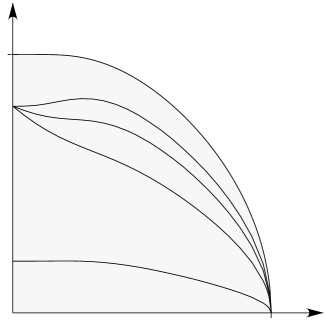
$h$$0.8$$0.2$$T_{c}$$T$$i$$ii$$iii$$iv$

Figure 2: A sequence of phase coexistence lines, separating the phase in which the interface is a straight line and the phase in which it is pinned to the wall, for different values of the parameters $a$ and $b$. For each of the four curves, for all values of the parameters $\beta$ and $h$ above the curve, the interface is the straight line and for all values of the parameters below the curve the interface is pinned to the wall. The shaded area correspond to the value of $(\beta,h)$ so that $\hat{\tau}_{\mathchoice{\mbox{$\displaystyle\rm\footnotesize bd$}}{\mbox{$\textstyle\rm\footnotesize bd$}}{\mbox{$\scriptstyle\rm\footnotesize bd$}}{\mbox{$\scriptscriptstyle\rm\footnotesize bd$}}}(\beta,h)<\hat{\tau}((1,0);\beta)$. The four curves correspond to: i) $a=0.1$, $b=0.1$; ii) $a=0.1$, $b=0.2$; iii) $a=0.1$, $b=0.4$; iv) $a=0.4$, $b=0.4$. Observe that the system in case 1) exhibits reentrance: if we fix the value of the magnetic field near $0.8$ and increase the temperature from 0 to $T_{c}$, the system changes from phase I to phase II and then to phase I again (see also Fig. 3).

         

$0.80$$0.78$$0.82$$1$$T$$h$$0.80$$0.78$$0.82$$1$$T$$h$

Figure 3: This figure shows part of the phase coexistence line for $a=0.1,b=0.1$ (left), and $a=0.1,b=0.12$ (right). For values of the parameters $\beta$ and $h$ below these curves the interface is pinned, while it is a straight line above these curves. In case 2) the system has even one more transition in temperature for $h$ slightly smaller than $0.8$.

4 Concentration properties

By duality, properties of interfaces at temperatures below $T_{c}$ are related to properties of the random–line representation of the two–point function of the Ising model at temperatures above $T_{c}$. The results of this section are given for the two–point function and are valid for all temperatures above the critical temperature $T_{c}$. Our concentration results are based on the sharp triangle inequality, which allows us to improve Propositions 6.1 and 6.2 of [PV1]. The results are essentially optimal.

The random–line representation for the two–point function $\langle\sigma(t)\sigma(t^{\prime})\rangle_{\Lambda_{L}^{*}}$ is the formula

$$\langle\sigma(t)\sigma(t^{\prime})\rangle_{\Lambda_{L}^{*}}=\sum_{\lambda:t\rightarrow t^{\prime}}q^{*}_{L}(\lambda)\,.$$ (4.1)

On the set of all open contours $\lambda$, such that $\delta\lambda=\{t,t^{\prime}\}$, $q^{*}_{L}(\lambda)$ defines a measure whose total mass is $\langle\sigma(t)\sigma(t^{\prime})\rangle_{\Lambda_{L}^{*}}$. The same is true for the similar representations of $\langle\sigma(t)\sigma(t^{\prime})\rangle(\beta^{*})$ or $\langle\sigma(t)\sigma(t^{\prime})\rangle_{{{\rm I\!L}}^{*}}$. It is therefore important to have good upper and lower bounds for these quantities. We recall some basic results. Proposition 4.1 is proven in [MW] and the last part in [PV1]; Proposition 4.2 is proven in [PV1].

We set $\Sigma^{*}:=\{x\in{{\rm I\!L}}^{*}:\,x(2)=-1/2\,\}$ and $\Sigma^{*}_{L}:=\Sigma^{*}\cap\Lambda^{*}_{L}$.

Proposition 4.1

Let $\beta^{*}<\beta_{c}$.

1. There exists $K$ such that

   $$\langle\sigma(x)\sigma(y)\rangle\geq K{\exp\{-\hat{\tau}(y-x)\}\over\|x-y\|^{1/2}}\,.$$ (4.2)

2. Let $\hat{\tau}(1,0)=\hat{\tau}_{\mathchoice{\mbox{$\displaystyle\rm\footnotesize bd$}}{\mbox{$\textstyle\rm\footnotesize bd$}}{\mbox{$\scriptstyle\rm\footnotesize bd$}}{\mbox{$\scriptscriptstyle\rm\footnotesize bd$}}}$ and $x,y\in\Sigma^{*}$. Then there exists $K^{\prime}$ such that

   $$\langle\sigma(x)\sigma(y)\rangle_{{\rm I\!L}^{*}}\geq K^{\prime}{\exp\{-\hat{\tau}_{\mathchoice{\mbox{$\displaystyle\rm\footnotesize bd$}}{\mbox{$\textstyle\rm\footnotesize bd$}}{\mbox{$\scriptstyle\rm\footnotesize bd$}}{\mbox{$\scriptscriptstyle\rm\footnotesize bd$}}}(y-x)\}\over\|x-y\|^{3/2}}\,.$$ (4.3)

3. Let $\hat{\tau}(1,0)>\hat{\tau}_{\mathchoice{\mbox{$\displaystyle\rm\footnotesize bd$}}{\mbox{$\textstyle\rm\footnotesize bd$}}{\mbox{$\scriptstyle\rm\footnotesize bd$}}{\mbox{$\scriptscriptstyle\rm\footnotesize bd$}}}$ and $x,y\in\Sigma^{*}$. Then there exists $C>0$ such that

   $$\langle\sigma(x)\sigma(y)\rangle_{{{\rm I\!L}}^{*}}\geq C\exp\{-\hat{\tau}_{\mathchoice{\mbox{$\displaystyle\rm\footnotesize bd$}}{\mbox{$\textstyle\rm\footnotesize bd$}}{\mbox{$\scriptstyle\rm\footnotesize bd$}}{\mbox{$\scriptscriptstyle\rm\footnotesize bd$}}}\|x-y\|\}\,.$$ (4.4)

Proposition 4.2

Let $\beta^{*}<\beta_{c}$ and $0<h^{*}<\infty$.

1. Let $x$, $y$ be two different points of ${{\mathchoice{\hbox{$\sf\textstyle Z\kern-3.99994ptZ$}}{\hbox{$\sf\textstyle Z\kern-3.99994ptZ$}}{\hbox{$\sf\scriptstyle Z\kern-2.10002ptZ$}}{\hbox{$\sf\scriptscriptstyle Z\kern-0.99998ptZ$}}}}^{2*}$. Then

   $$\langle\sigma(x)\sigma(y)\rangle=\sum_{\lambda:x\rightarrow y}q^{*}(\lambda)\leq\exp\{-\hat{\tau}(y-x)\}\,.$$ (4.5)

2. Let $x$, $y$ be two different points of $\Sigma^{*}_{L}$. Then

   $$\langle\sigma(x)\sigma(y)\rangle_{\Lambda_{L}^{*}}\leq\langle\sigma(x)\sigma(y)\rangle_{{{\rm I\!L}}^{*}}=\sum_{\lambda:x\rightarrow y}q^{*}_{{{\rm I\!L}}^{*}}(\lambda)\leq\exp\{-\hat{\tau}_{\mathchoice{\mbox{$\displaystyle\rm\footnotesize bd$}}{\mbox{$\textstyle\rm\footnotesize bd$}}{\mbox{$\scriptstyle\rm\footnotesize bd$}}{\mbox{$\scriptscriptstyle\rm\footnotesize bd$}}}\cdot\|y-x)\|\}\,.$$ (4.6)

3. Let $x$, $y$ be two different points of $\Lambda_{L}^{*}$. Then

   $$\sum_{{\lambda:x\rightarrow y\atop\lambda\cap{\cal E}^{*}(\Sigma^{*})=\emptyset}}q_{L}^{*}(\lambda;\beta^{*},h^{*})\leq\langle\sigma(x)\sigma(y)\rangle(\beta^{*})\,.$$ (4.7)

4. Let $x$, $y$, $z$ be three different points of $\Lambda_{L}^{*}$. Then

   $$\sum_{{\scriptstyle\lambda:x\rightarrow z\atop\scriptstyle y\ni\lambda}}q_{L}^{*}(\lambda)\leq\sum_{\lambda:x\rightarrow y}q_{L}^{*}(\lambda)\sum_{\lambda:y\rightarrow z}q_{L}^{*}(\lambda)\,.$$ (4.8)

Remark: Statement 4. of Proposition 4.2 can be written as

$$\sum_{{\scriptstyle\lambda:x\rightarrow z\atop\scriptstyle y\ni\lambda}}q_{L}^{*}(\lambda)\leq\langle\sigma(x)\sigma(y)\rangle_{\Lambda_{L}^{*}}\,\langle\sigma(y)\sigma(z)\rangle_{\Lambda_{L}^{*}}\,.$$ (4.9)

There are variants of 4.. Let $\lambda:x\rightarrow z$ and $y\in\lambda$; let $\lambda_{1}$ be the part of $\lambda$ from $x$ to $y$ and $\lambda_{2}$ be the part of $\lambda$ from $y$ to $z$. Then

$$\sum_{{\scriptstyle\lambda:x\rightarrow z\,,y\ni\lambda\atop\scriptstyle\lambda_{1}\cap{\cal E}^{*}(\Sigma^{*})=\emptyset}}q_{L}^{*}(\lambda;\beta^{*},h^{*})\leq\langle\sigma(x)\sigma(y)\rangle_{\Lambda_{L}^{*}}(\beta^{*},1)\,\langle\sigma(y)\sigma(z)\rangle_{\Lambda_{L}^{*}}(\beta^{*},h^{*})\,.$$ (4.10)

or

$$\sum_{{{\scriptstyle\lambda:x\rightarrow z\,,y\ni\lambda\atop\scriptstyle\lambda_{1}\cap{\cal E}^{*}(\Sigma^{*})=\emptyset}\atop\scriptstyle\lambda_{2}\cap{\cal E}^{*}(\Sigma^{*})=\emptyset}}q_{L}^{*}(\lambda;\beta^{*},h^{*})\leq\langle\sigma(x)\sigma(y)\rangle_{\Lambda_{L}^{*}}(\beta^{*},1)\,\langle\sigma(y)\sigma(z)\rangle_{\Lambda_{L}^{*}}(\beta^{*},1)\,.$$ (4.11)

We prove Propositions 4.3 to 4.5, which state concentration properties of the random lines contributing to the two-point function. Given $x$, $y\in{{\mathchoice{\hbox{$\sf\textstyle Z\kern-3.99994ptZ$}}{\hbox{$\sf\textstyle Z\kern-3.99994ptZ$}}{\hbox{$\sf\scriptstyle Z\kern-2.10002ptZ$}}{\hbox{$\sf\scriptscriptstyle Z\kern-0.99998ptZ$}}}}^{2*}$ and $\rho>0$ we set

$${\cal S}(x,y;\rho):=\{t\in{{\mathchoice{\hbox{$\sf\textstyle Z\kern-3.99994ptZ$}}{\hbox{$\sf\textstyle Z\kern-3.99994ptZ$}}{\hbox{$\sf\scriptstyle Z\kern-2.10002ptZ$}}{\hbox{$\sf\scriptscriptstyle Z\kern-0.99998ptZ$}}}}^{2*}\,:\,\|t-x\|+\|t-y\|\leq\|y-x\|+\rho\}\,,$$ (4.12)

and $\partial{\cal S}(x,y;\rho)$ is the set of $z\in{{\mathchoice{\hbox{$\sf\textstyle Z\kern-3.99994ptZ$}}{\hbox{$\sf\textstyle Z\kern-3.99994ptZ$}}{\hbox{$\sf\scriptstyle Z\kern-2.10002ptZ$}}{\hbox{$\sf\scriptscriptstyle Z\kern-0.99998ptZ$}}}}^{2*}\backslash{\cal S}(x,y;\rho)$ such that there exists an edge $\langle z,z^{\prime}\rangle$ with $z^{\prime}\in{\cal S}(x,y;\rho)$.

Proposition 4.3

Let $x$, $y\in\Lambda_{L}^{*}$ and $\rho>0$. Let ${\cal S}_{1}:={\cal S}(x,y;\rho)$. Then ($\Delta$ is defined in (2.20) and (2.21))

$$\sum_{{{\scriptstyle\lambda:\,x\mapsto y\atop\scriptstyle\lambda\not\subset{\cal E}^{*}({\cal S}_{1})}\atop\scriptstyle\lambda\cap{\cal E}^{*}({\cal S}_{1})\cap{\cal E}^{*}(\Sigma^{*}_{L})=\emptyset}}q_{L}^{*}(\lambda)\leq|\partial{\cal S}_{1}|\exp\{-\Delta\rho\}\exp\{-\hat{\tau}(y-x)\}$$ (4.13)

$$+\sum_{z_{1},z_{2}\in\Sigma^{*}_{L}}\exp\{-\hat{\tau}(z_{1}-x)\}\exp\{-\hat{\tau}_{\mathchoice{\mbox{$\displaystyle\rm\footnotesize bd$}}{\mbox{$\textstyle\rm\footnotesize bd$}}{\mbox{$\scriptstyle\rm\footnotesize bd$}}{\mbox{$\scriptscriptstyle\rm\footnotesize bd$}}}(z_{2}-z_{1})\}\exp\{-\hat{\tau}(y-z_{2})\}\,.$$

Proof. Let $s\mapsto\lambda(s)$ be a parameterization of the open contour $\lambda$ from $x$ to $y$. Let $s_{1}$ be the first time (if any) such that $\lambda(s_{1})\in\Sigma^{*}_{L}$ and $s_{2}$ the last time such that $\lambda(s_{2})\in\Sigma^{*}_{L}$.

$$\sum_{{{\scriptstyle\lambda:\,x\mapsto y\atop\scriptstyle\lambda\not\subset{\cal E}^{*}({\cal S}_{1})}\atop\scriptstyle\lambda\cap{\cal E}^{*}({\cal S}_{1})\cap{\cal E}^{*}(\Sigma^{*}_{L})=\emptyset}}q_{L}^{*}(\lambda) \leq \sum_{t\in\partial{\cal S}_{1}}\sum_{{\scriptstyle\lambda:x\rightarrow y\,,\lambda\ni t\atop\scriptstyle\lambda\cap{\cal E}^{*}(\Sigma^{*}_{L})=\emptyset}}q_{L}^{*}(\lambda)$$

$$+ \sum_{z_{1},z_{2}\in\Sigma^{*}_{L}}\sum_{{\scriptstyle\lambda:x\rightarrow y\atop\scriptstyle\lambda(s_{1})=z_{1},\lambda(s_{2})=z_{2}}}q_{L}^{*}(\lambda)\,.$$

Using Proposition 4.2, the remark following it and the sharp triangle inequality, we get

$$\sum_{t\in\partial{\cal S}_{1}}\sum_{{\scriptstyle\lambda:x\rightarrow y\,,\lambda\ni t\atop\scriptstyle\lambda\cap{\cal E}^{*}(\Sigma^{*}_{L})=\emptyset}}q_{L}^{*}(\lambda) \leq \sum_{t\in\partial{\cal S}_{1}}\langle\sigma(x)\sigma(t)\rangle_{\Lambda_{L}^{*}}(\beta^{*},1)\,\langle\sigma(t)\sigma(y)\rangle_{\Lambda_{L}^{*}}(\beta^{*},1)$$

$$\leq \sum_{t\in\partial{\cal S}_{1}}\exp\{-(\hat{\tau}(t-x)+\hat{\tau}(y-t))\}$$

$$\leq \sum_{t\in\partial{\cal S}_{1}}\exp\{-(\hat{\tau}(y-x)+\Delta\rho)\}$$

$$\leq |\partial{\cal S}_{1}|\exp\{-\Delta\rho\}\exp\{-\hat{\tau}(y-x)\}\,,$$

and

$$\sum_{z_{1},z_{2}\in\Sigma^{*}_{L}}\sum_{{\scriptstyle\lambda:x\rightarrow y\atop\scriptstyle\lambda(s_{1})=z_{1},\lambda(s_{2})=z_{2}}}q_{L}^{*}(\lambda) \leq \sum_{z_{1},z_{2}\in\Sigma^{*}_{L}}\exp\{-\hat{\tau}(z_{1}-x)\}$$

$$\cdot\exp\{-\hat{\tau}_{\mathchoice{\mbox{$\displaystyle\rm\footnotesize bd$}}{\mbox{$\textstyle\rm\footnotesize bd$}}{\mbox{$\scriptstyle\rm\footnotesize bd$}}{\mbox{$\scriptscriptstyle\rm\footnotesize bd$}}}(z_{2}-z_{1})\}\exp\{-\hat{\tau}(y-z_{2})\}\,.$$

$\sqcap$$\sqcup$

Remarks.

1. If $h^{*}\leq 1$, then the statement (4.13) simplifies,

$$\sum_{{\scriptstyle\lambda:x\mapsto y\atop\scriptstyle\lambda\not\subset{\cal E}^{*}({\cal S}_{1})}}q_{L}^{*}(\lambda)\leq|\partial{\cal S}_{1}|\exp\{-\Delta\rho\}\exp\{-\hat{\tau}(y-x)\}\,.$$ (4.17)

2. At the thermodynamical limit we can improve (4.17) using Proposition 4.1.

$$\sum_{{\scriptstyle\lambda:x\mapsto y\atop\scriptstyle\lambda\not\subset{\cal E}^{*}({\cal S}_{1})}}q^{*}(\lambda)\leq{1\over K}|\partial{\cal S}_{1}|\|x-y\|^{1/2}\exp\{-\Delta\rho\}\langle\sigma(x)\sigma(y)\rangle\,.$$ (4.18)

The replacement of $\exp\{-\hat{\tau}(y-x)\}$ by $\langle\sigma(x)\sigma(y)\rangle$ is significant since $\langle\sigma(x)\sigma(y)\rangle$ is the total mass of the measure defined by $q^{*}(\lambda)$ on the set of all $\lambda$ with $\delta\lambda=\{x,y\}$.

3. If $1<h^{*}<h^{*}_{c}$, then the sharp triangle inequality applied two times to (4.13) gives

$$\sum_{{{\scriptstyle\lambda:\,x\mapsto y\atop\scriptstyle\lambda\not\subset{\cal E}^{*}({\cal S}_{1})}\atop\scriptstyle\lambda\cap{\cal E}^{*}({\cal S}_{1})\cap{\cal E}^{*}(\Sigma^{*}_{L})=\emptyset}}q_{L}^{*}(\lambda)\leq\exp\{-\hat{\tau}(y-x)\}\Big{(}|\partial{\cal S}_{1}|\exp\{-\Delta\rho\}$$ (4.19)

$$+\sum_{z_{1},z_{2}\in\Sigma^{*}_{L}}\exp\{-\Delta(\|z_{1}-x\|+\|z_{2}-z_{1}\|+\|y-z_{2}\|-\|x-y\|)\}\Big{)}\,.$$

Proposition 4.4

Let $x$, $y\in\Lambda_{L}^{*}$ with $x(2)=y(2)=-1/2$, and $\rho>0$. Let ${\cal S}_{2}:={\cal S}(x,y;\rho)$. If $\hat{\tau}(1,0)=\hat{\tau}_{\mathchoice{\mbox{$\displaystyle\rm\footnotesize bd$}}{\mbox{$\textstyle\rm\footnotesize bd$}}{\mbox{$\scriptstyle\rm\footnotesize bd$}}{\mbox{$\scriptscriptstyle\rm\footnotesize bd$}}}$, that is $h^{*}\leq h^{*}_{c}$, then

$$\sum_{{\scriptstyle\lambda:x\mapsto y\atop\scriptstyle\lambda\not\subset{\cal E}^{*}({\cal S}_{2})}}q^{*}_{L}(\lambda)\leq O(\|x-y\|+\rho)|\partial{\cal S}_{2}|\exp\{-\Delta\rho\}\exp\{-\hat{\tau}(y-x)\}\,.$$ (4.20)

Proof. If $\hat{\tau}(1,0)=\hat{\tau}_{\mathchoice{\mbox{$\displaystyle\rm\footnotesize bd$}}{\mbox{$\textstyle\rm\footnotesize bd$}}{\mbox{$\scriptstyle\rm\footnotesize bd$}}{\mbox{$\scriptscriptstyle\rm\footnotesize bd$}}}$ and $u$, $v\in{\rm I\!L}^{*}$ with $u(2)=v(2)=-1/2$, then

$$\hat{\tau}_{\mathchoice{\mbox{$\displaystyle\rm\footnotesize bd$}}{\mbox{$\textstyle\rm\footnotesize bd$}}{\mbox{$\scriptstyle\rm\footnotesize bd$}}{\mbox{$\scriptscriptstyle\rm\footnotesize bd$}}}\|u-v\|=\hat{\tau}(u-v)\,.$$ (4.21)

Let $\lambda:x\mapsto y$, with $\lambda\ni t$, $t\in\partial{\cal S}_{2}$. We consider $\lambda$ as a parameterized curve, $s\mapsto\lambda(s)$, from $x$ to $y$. We set $t=\lambda(s^{*})$; we denote by $s_{1}$ the last time before $s^{*}$ such that $\lambda(s_{1})\in\Sigma^{*}_{L}$; we denote by $s_{2}$ the first time after $s^{*}$ such that $\lambda(s_{2})\in\Sigma^{*}_{L}$. We have

$$\sum_{\lambda:x\rightarrow y\atop\lambda\not\subset{\cal E}^{*}({\cal S}_{2})}q^{*}_{L}(\lambda) \leq \sum_{t\in\partial{\cal S}_{2}}\sum_{\lambda:x\rightarrow y\atop\lambda\ni t}q^{*}_{L}(\lambda)$$

$$\leq \sum_{t\in\partial{\cal S}_{2}}\sum_{u,v\in\Sigma^{*}_{L}}\sum_{{\scriptstyle\lambda:x\rightarrow y\,,t\in\lambda\atop\scriptstyle\lambda(s_{1})=u,\lambda(s_{2})=v}}q^{*}_{L}(\lambda)\,.$$

Using (4.21), Proposition 4.2, GKS inequalities and the sharp triangle inequality, we get

$$\sum_{u,v}\sum_{\lambda:x\rightarrow y\atop\lambda\ni u,t,v}q^{*}_{L} \leq \sum_{u,v}\langle\sigma(x)\sigma(u)\rangle_{{\rm I\!L}^{*}}\langle\sigma(u)\sigma(t)\rangle\langle\sigma(t)\sigma(v)\rangle\langle\sigma(v)\sigma(y)\rangle_{{\rm I\!L}^{*}}$$

$$\leq \sum_{u,v}\exp\{-\hat{\tau}(u-x)-\hat{\tau}(t-u)\}\exp\{-\hat{\tau}(v-t)-\hat{\tau}(y-v)\}$$

$$\leq \sum_{u,v}\exp\{-\hat{\tau}(t-x)\}\exp\{-\Delta(\|x-u\|+\|u-t\|-\|x-t\|)\}$$

$$\cdot\exp\{-\hat{\tau}(y-t)\}\exp\{-\Delta(\|y-v\|+\|v-t\|-\|y-t\|)\}$$

$$\leq O(\|x-y\|+\rho)\exp\{-(\hat{\tau}(t-x)+\hat{\tau}(y-t))\}\,.$$

Then the proof is as in (4). $\sqcap$$\sqcup$

In the case of partial wetting, i.e. $\hat{\tau}(1,0)>\hat{\tau}_{\mathchoice{\mbox{$\displaystyle\rm\footnotesize bd$}}{\mbox{$\textstyle\rm\footnotesize bd$}}{\mbox{$\scriptstyle\rm\footnotesize bd$}}{\mbox{$\scriptscriptstyle\rm\footnotesize bd$}}}(1,0)$, the previous proposition can be improved to reflect the fact that the contours stick to the wall, even microscopically.

Proposition 4.5

Suppose $h^{*}>h_{c}^{*}$ (partial wetting for the dual model). Let $x$, $y\in\Lambda^{*}_{L}$ with $x(2)=y(2)=-1/2$, $x(1)<y(1)$, and let $\rho_{i}>0$, $i=1,2$. Let

$${\cal S}_{3}:=\{t\in\Lambda^{*}_{L}\,:\,x(1)-\rho_{1}\leq t(1)\leq y(1)+\rho_{1}\,,\,-1/2\leq t(2)\leq\rho_{2}\}\,.$$ (4.23)

Then, there exists a constant $\overline{C}(\beta)>0$ such that

$$\sum_{{\scriptstyle\lambda:x\rightarrow y\atop\scriptstyle\lambda\not\subset{\cal E}^{*}({\cal S}_{3})}}q^{*}_{L}(\lambda)\leq|\partial{\cal S}_{3}|\Big{(}\exp\{-2\rho_{1}\hat{\tau}_{\mathchoice{\mbox{$\displaystyle\rm\footnotesize bd$}}{\mbox{$\textstyle\rm\footnotesize bd$}}{\mbox{$\scriptstyle\rm\footnotesize bd$}}{\mbox{$\scriptscriptstyle\rm\footnotesize bd$}}}\}+|\rho_{2}|\exp\{-\overline{C}\rho_{2}\}\Big{)}\exp\{-\hat{\tau}_{\mathchoice{\mbox{$\displaystyle\rm\footnotesize bd$}}{\mbox{$\textstyle\rm\footnotesize bd$}}{\mbox{$\scriptstyle\rm\footnotesize bd$}}{\mbox{$\scriptscriptstyle\rm\footnotesize bd$}}}\|y-x\|\}\,.$$ (4.24)

Proof. Let $\partial{\cal S}_{3}:=\{t\in{\cal S}_{3}\,:\,t(2)=\rho_{2}\mbox{ or }t(1)=x(1)-\rho_{1}\mbox{ or }t(1)=y(1)+\rho_{1}\}$; we can write

$$\sum_{\scriptstyle\lambda:x\rightarrow y\atop\scriptstyle\lambda\not\subset{\cal E}^{*}({\cal S}_{3})}q^{*}_{L}(\lambda) \leq \sum_{t\in\partial{\cal S}_{3}}\sum_{\scriptstyle\lambda:x\rightarrow y\atop\scriptstyle\lambda\ni t}q^{*}_{L}(\lambda)$$

$$\leq \sum_{\scriptstyle t\in\partial{\cal S}_{3}\atop\scriptstyle t(2)<\rho_{2}}\sum_{\scriptstyle\lambda:x\rightarrow y\atop\scriptstyle\lambda\ni t}q^{*}_{L}(\lambda)+\sum_{\scriptstyle t\in\partial{\cal S}_{3}\atop\scriptstyle t(2)=\rho_{2}}\sum_{\scriptstyle\lambda:x\rightarrow y\atop\scriptstyle\lambda\ni t}q^{*}_{L}(\lambda)\,.$$

We treat these sums separately. By symmetry and GKS inequalities

$$\sum_{t\in\partial{\cal S}_{3}\atop t(2)<\rho_{2}}\sum_{\lambda:x\rightarrow y\atop\lambda\ni t}q^{*}_{L}(\lambda) \leq 2\sum_{\scriptstyle t\in\partial{\cal S}_{3}\atop\scriptstyle t(1)=x(1)-\rho_{1}}\langle\sigma_{x}\sigma_{t}\rangle_{{\rm I\!L}^{*}}\langle\sigma_{t}\sigma_{y}\rangle_{{\rm I\!L}^{*}}$$

$$= 2\sum_{\scriptstyle t\in\partial{\cal S}_{3}\atop\scriptstyle t(1)=x(1)-\rho_{1}}\langle\sigma_{\overline{x}}\sigma_{t}\rangle_{{\rm I\!L}^{*}}\langle\sigma_{t}\sigma_{y}\rangle_{{\rm I\!L}^{*}}$$

$$\leq 2\sum_{\scriptstyle t\in\partial{\cal S}_{3}\atop\scriptstyle t(1)=x(1)-\rho_{1}}\langle\sigma_{\overline{x}}\sigma_{y}\rangle_{{\rm I\!L}^{*}}$$

$$\leq 2\sum_{\scriptstyle t\in\partial{\cal S}_{3}\atop\scriptstyle t(1)=x(1)-\rho_{1}}\exp\{-2\rho_{1}\hat{\tau}_{\mathchoice{\mbox{$\displaystyle\rm\footnotesize bd$}}{\mbox{$\textstyle\rm\footnotesize bd$}}{\mbox{$\scriptstyle\rm\footnotesize bd$}}{\mbox{$\scriptscriptstyle\rm\footnotesize bd$}}}\}\exp\{-\hat{\tau}_{\mathchoice{\mbox{$\displaystyle\rm\footnotesize bd$}}{\mbox{$\textstyle\rm\footnotesize bd$}}{\mbox{$\scriptstyle\rm\footnotesize bd$}}{\mbox{$\scriptscriptstyle\rm\footnotesize bd$}}}\|y-x\|\}\,,$$

where $\overline{x}$ is the image of $x$ under a reflection of axis $\{u\,:\,u(1)=t(1)\}$.

Let $t\in\lambda$ and $t(2)=\rho_{2}$. As above $\lambda$ is considered as a parameterized curve, and we set $t=\lambda(s^{*})$; we denote by $s_{1}$ the last time before $s^{*}$ such that $\lambda(s_{1})\in\Sigma^{*}_{L}$; we denote by $s_{2}$ the first time after $s^{*}$ such that $\lambda(s_{2})\in\Sigma^{*}_{L}$. As above we get ($u=\lambda(s_{1})$, $v=\lambda(s_{2})$)

$$\sum_{\scriptstyle t\in\partial{\cal S}_{3}\atop\scriptstyle t(2)=\rho_{2}}\sum_{\lambda:x\rightarrow y\atop\lambda\ni t}q^{*}_{L}(\lambda) \leq \sum_{\scriptstyle t\in\partial{\cal S}_{3}\atop\scriptstyle t(2)=\rho_{2}}\sum_{u,v}\langle\sigma_{x}\sigma_{u}\rangle_{{\rm I\!L}^{*}}\langle\sigma_{u}\sigma_{t}\rangle\langle\sigma_{t}\sigma_{v}\rangle\langle\sigma_{v}\sigma_{y}\rangle_{{\rm I\!L}^{*}}$$

$$\leq \sum_{\scriptstyle t\in\partial{\cal S}_{3}\atop\scriptstyle t(2)=\rho_{2}}\sum_{u,v}\exp\{-\hat{\tau}_{\mathchoice{\mbox{$\displaystyle\rm\footnotesize bd$}}{\mbox{$\textstyle\rm\footnotesize bd$}}{\mbox{$\scriptstyle\rm\footnotesize bd$}}{\mbox{$\scriptscriptstyle\rm\footnotesize bd$}}}(\|u-x\|+\|y-v\|)\}$$

$$\cdot\exp\{-\hat{\tau}(t-u)-\hat{\tau}(v-t)\}$$

$$\leq \sum_{\scriptstyle t\in\partial{\cal S}_{3}\atop\scriptstyle t(2)=\rho_{2}}\sum_{u,v}\exp\{-\hat{\tau}_{\mathchoice{\mbox{$\displaystyle\rm\footnotesize bd$}}{\mbox{$\textstyle\rm\footnotesize bd$}}{\mbox{$\scriptstyle\rm\footnotesize bd$}}{\mbox{$\scriptscriptstyle\rm\footnotesize bd$}}}(\|u-x\|+\|y-v\|)\}$$

$$\cdot\exp\{-\hat{\tau}(u-v)\}\exp\{-\Delta(\|u-t\|+\|t-v\|-\|u-v\|)\}$$

$$\leq \sum_{\scriptstyle t\in\partial{\cal S}_{3}\atop\scriptstyle t(2)=\rho_{2}}\sum_{u,v}\exp\{-\hat{\tau}_{\mathchoice{\mbox{$\displaystyle\rm\footnotesize bd$}}{\mbox{$\textstyle\rm\footnotesize bd$}}{\mbox{$\scriptstyle\rm\footnotesize bd$}}{\mbox{$\scriptscriptstyle\rm\footnotesize bd$}}}\|x-y\|\}\exp\{-(\hat{\tau}(1,0)-\hat{\tau}_{\mathchoice{\mbox{$\displaystyle\rm\footnotesize bd$}}{\mbox{$\textstyle\rm\footnotesize bd$}}{\mbox{$\scriptstyle\rm\footnotesize bd$}}{\mbox{$\scriptscriptstyle\rm\footnotesize bd$}}})\|u-v\|\}$$

$$\cdot\exp\{-\Delta(\|u-t\|+\|t-v\|-\|u-v\|)\}\,,$$

The conclusion follows from the observations: 1. the summation is over the base of the triangle $uvt$; 2. the term $\exp\{-(\hat{\tau}(1,0)-\hat{\tau}_{\mathchoice{\mbox{$\displaystyle\rm\footnotesize bd$}}{\mbox{$\textstyle\rm\footnotesize bd$}}{\mbox{$\scriptstyle\rm\footnotesize bd$}}{\mbox{$\scriptscriptstyle\rm\footnotesize bd$}}})\|u-v\|\}$ allows to control the triangles with a large base, while the term $\exp\{-\Delta(\|u-t\|+\|t-v\|-\|u-v\|)\}$ can be used to control the terms in which the base is far from the point $t$. $\sqcap$$\sqcup$

5 Probability of the phase separation line

We study the probability of the phase separation line by making a coarse–grained description of it. We estimate in terms of its surface tension the probability that a given coarse–grained description occurs.

We first prove an essential lower bound and then proceed with the main estimate.

Proposition 5.1

Let $\beta>\beta_{c}$, $h>0$, $0<a<1$, $0<b<1$ and ${\tt W}^{*}={\tt W}^{*}(\beta,h)$ be the minimum of the functional ${\tt W}$. Then there exists $C>0$ and $L_{0}=L_{0}(\beta,h)$ such that, for all $L\geq L_{0}$,

$$Z^{ab}(\Lambda_{L})\geq{\exp\{-{\tt W}^{*}L\}\over L^{C}}Z^{-}(\Lambda_{L})\,.$$ (5.1)

Remark. The dual statement of Proposition 5.1 is

$$\langle\sigma(t_{l}^{L})\sigma(t_{r}^{L})\rangle_{\Lambda_{L}^{*}}\geq{\exp\{-{\tt W}^{*}L\}\over L^{C}}\,.$$ (5.2)

Proof. We can write, using Proposition 2.3,

$$Z^{ab}(\Lambda_{L})=Z^{-}(\Lambda_{L})\sum_{\scriptstyle\lambda:\atop\scriptstyle\delta\lambda=\{t_{l}^{L},t_{r}^{L}\}}q^{*}_{L}(\lambda)\,.$$ (5.3)

Let ${\cal C}^{*}$ be the simple rectifiable curve in $Q$ which realizes the minimum of the variational problem (or one of the minima in case of degeneracy). Let $K_{1}>0$, which will be chosen large enough below.

We first consider the case ${\cal C}^{*}={\cal D}$. Let $u^{L}_{l}$ and $u^{L}_{r}$ be the points of $\Lambda_{L}^{*}$ with $u_{l}^{L}(1)=t_{l}^{L}(1)+[K_{1}\log L]$, $u_{r}^{L}(1)=t_{r}^{L}(1)-[K_{1}\log L]$, which are closest to the straight line from $t_{l}^{L}$ to $t_{r}^{L}$.

We need the following result

Lemma 5.1

Let ${\cal B}$ be a rectangular box in $\Lambda_{L}^{*}$, and $x$, $y$ two points on its boundary. Let $d>0$ and $u$, $v$ be two points in ${\cal B}$ such that $u$ and $v$ are closest to the straight line from $x$ to $y$ and $\|x-u\|=\|y-v\|=d$. If the distance of ${\cal B}$ to $\Sigma^{*}_{L}$ is larger than $C^{\prime}\log L$, with $C^{\prime}>2$, then

$$\sum_{\lambda:x\rightarrow y\atop\lambda\subset{\cal E}^{*}({\cal B})}q^{*}_{L}(\lambda)\geq\exp\{-O(\log L)\}\sum_{\lambda:u\rightarrow v\atop\lambda\subset{\cal E}^{*}({\cal B})}q^{*}(\lambda)\,.$$ (5.4)

Proof. Following the proof of Proposition 6.1 of [PV1], from (6.38) to (6.42), we get

$$\sum_{\lambda:x\rightarrow y\atop\lambda\subset{\cal E}^{*}({\cal B})}q^{*}_{L}(\lambda)\geq\exp\{-O(\log L)\}\sum_{\lambda:u\rightarrow v\atop\lambda\subset{\cal E}^{*}({\cal B})}q^{*}_{L}(\lambda)\,.$$ (5.5)

Since the distance of ${\cal B}$ to $\Sigma^{*}$ is larger than $C^{\prime}\log L$ and $C^{\prime}>2$, then it follows from point 4. of Lemma 5.3 in [PV1] that there exists a constant $\tilde{C}>0$ such that for $L$ large enough and all $\lambda\subset{\cal E}^{*}({\cal B})$

$$q^{*}_{L}(\lambda)\geq q^{*}_{{{\rm I\!L}}^{*}}(\lambda)\geq\tilde{C}q^{*}(\lambda)\,.$$ (5.6)

This proves the lemma. $\sqcap$$\sqcup$

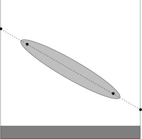
${\cal S}_{1}$$\Lambda^{*}_{L}$${\cal B}$$t_{l}^{L}$$t_{r}^{L}$$u_{r}^{L}$$u_{l}^{L}$

Figure 4: The ellipse ${\cal S}_{1}$; the box ${\cal B}$ is the whole box minus the bottom strip.

Let $C^{\prime}>2$. We introduce ${\cal B}:=\{t\in\Lambda_{L}^{*}\,:\,t(2)>[C^{\prime}\log L]\}$. Let ${\cal S}_{1}$ be the elliptical set of Proposition 4.3 with $x=u_{l}^{L}$, $y=u_{r}^{L}$, $\rho=O(K_{1}\log L)$ so that ${\cal E}^{*}({\cal S}_{1})\subset{\cal E}^{*}({\cal B})$ (see Fig. 4). From Lemma 5.1, applied to the box ${\cal B}$ with $x=t_{l}^{L}$, $y=t_{r}^{L}$ , $u=u_{l}^{L}$ and $v=v_{l}^{L}$, and the second remark following Proposition 4.3, we get

$${Z^{ab}(\Lambda_{L})\over Z^{-}(\Lambda_{L})} \geq \sum_{\lambda:t_{l}^{L}\rightarrow t_{r}^{L}\atop\lambda\subset{\cal E}^{*}({\cal B})}q^{*}_{L}(\lambda)$$

$$\geq \exp\{-O(\log L)\}\sum_{\lambda:u_{l}^{L}\rightarrow u_{r}^{L}\atop\lambda\subset{\cal E}^{*}({\cal S}_{1})}q^{*}(\lambda)$$

$$\geq \exp\{-O(\log L)\}\Big{(}\sum_{\lambda:u_{l}^{L}\rightarrow u_{r}^{L}}q^{*}(\lambda)-\sum_{\lambda:u_{l}^{L}\rightarrow u_{r}^{L}\atop\lambda\not\subset{\cal E}^{*}({\cal S}_{1})}q^{*}(\lambda)\Big{)}$$

$$\geq \exp\{-O(\log L)\}\langle\sigma(u_{l}^{L})\sigma(u_{r}^{L})\rangle\Big{(}1-{1\over K}|\partial{\cal S}_{1}|\,\|u_{l}^{L}-u_{r}^{L}\|^{1/2}\exp\{-\Delta\rho\}\Big{)}$$

$$\geq {\exp\{-\hat{\tau}(t_{l}^{L}-t_{r}^{L})\}\over L^{C}}\,,$$

for some positive constant $C$, by taking $K_{1}$ large enough.

We now consider the case ${\cal C}^{*}={\cal W}$. Since $h>0$, the angle $\theta_{Y}$ satisfies $0<\theta_{Y}<\pi/2$. Denote by $w_{1}^{L}$ and $w_{2}^{L}$ the two points on $\Sigma^{*}_{L}$ which are closest to the corners of the polygonal line ${\cal W}$ scaled by $L$.

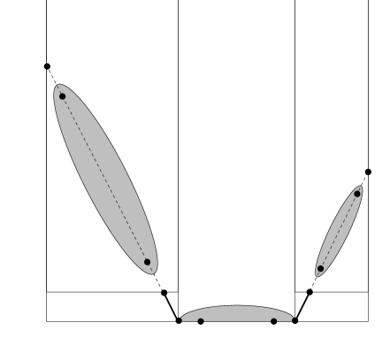
${w^{\prime}_{1}}{}^{L}$$v_{l}^{L}$${w^{\prime}_{2}}{}^{L}$$v_{r}^{L}$$t_{l}^{L}$$t_{r}^{L}$$w_{2}^{L}$$u_{l}^{L}$$u_{r}^{L}$$w_{1}^{L}$$\Lambda_{L}^{*}$${\cal B}_{1}$${\cal B}_{2}$${\cal B}_{3}$${\cal S}_{1}$${\cal S}_{2}$${\cal S}_{3}$$r_{2}^{L}$$r_{1}^{L}$

Figure 5: The three boxes ${\cal B}_{i}$, $i=1,\dots,3$ and their elliptical subsets; the two bold segments represent the two shortest contours $\overline{\lambda}_{i}$, $i=1,2$.

We define three rectangular boxes (see Fig. 5)

$${{\cal B}}_{1} = \{t\in\Lambda_{L}^{*}\,:\,t(1)\leq w_{1}^{L}(1)\,,\,t(2)>[C^{\prime}\log L]\}\,,$$ (5.8)

$${{\cal B}}_{2} = \{t\in\Lambda_{L}^{*}\,:\,w_{1}^{L}(1)\leq t(1)\leq w_{2}^{L}(1)\}\,,$$ (5.9)

$${{\cal B}}_{3} = \{t\in\Lambda_{L}^{*}\,:\,w_{2}^{L}(1)\leq t(1)\,,\,t(2)>[C^{\prime}\log L]\}\,.$$ (5.10)

Moreover let $r_{1}^{L}$, resp. $r_{2}^{L}$, be the point of $\Lambda_{L}^{*}$ closest to the straight line through $t_{l}^{L}$ and $w_{1}^{L}$, resp. $t_{r}^{L}$ and $w_{2}^{L}$, such that $r_{1}^{L}(2)=[C^{\prime}\log L]+1/2$, resp. $r_{2}^{L}(2)=[C^{\prime}\log L]+1/2$. Let $\overline{\lambda}_{1}$, resp. $\overline{\lambda}_{2}$, be a shortest open contour from $r^{L}_{1}$ to $w^{L}_{1}$, resp. from $r^{L}_{2}$ to $w^{L}_{2}$. We define ${\cal A}$ as the set ${\cal A}$ of open contours $\lambda=\lambda_{1}\cup\overline{\lambda}_{1}\cup\lambda_{2}\cup\overline{\lambda_{2}}\cup\lambda_{3}$ such that

• $\lambda_{i}\subset{\cal E}^{*}({\cal B}_{i})$, $i=1,\dots,3$;

• $\lambda_{1}$ : $t_{l}^{L}\rightarrow r_{1}^{L}$;

• $\lambda_{2}$ : $w_{1}^{L}\rightarrow w_{2}^{L}$;

• $\lambda_{3}$ : $r_{2}^{L}\rightarrow t_{r}^{L}$.

We can write

$${Z^{ab}(\Lambda_{L})\over Z^{-}(\Lambda_{L})} \geq \sum_{\lambda\in{\cal A}}q^{*}_{L}(\lambda)$$ (5.11)

$$\geq \exp\{-O(\log L)\}\prod_{i}\sum_{\scriptstyle\lambda_{i}\subset{\cal E}^{*}({\cal B}_{i}):\atop\scriptstyle\lambda_{i}\,\mbox{\scriptsize as above}}q^{*}_{L}(\lambda_{i})\,.$$

We apply Lemma 5.1 to the sum over $\lambda_{1}$ with ${\cal B}={\cal B}_{1}$, $x=t_{l}^{L}$, $y=r_{1}^{L}$, $d=K_{1}\log L$; we denote by $u_{l}^{L}$ and $v_{l}^{L}$ the corresponding points $u$ and $v$. We apply the same lemma to the sum over $\lambda_{3}$ with ${\cal B}={\cal B}_{2}$, $x=r_{2}^{L}$, $y=t_{r}^{L}$, $d=K_{1}\log L$; we denote by $u_{r}^{L}$ and $v_{r}^{L}$ the corresponding points $u$ and $v$. The sum over $\lambda_{2}$ is taken care of by the following

Lemma 5.2

Let ${w_{1}^{\prime}}{}^{L}:=w_{1}^{L}+([K_{1}\log L],0)$, $w^{\prime}_{2}{}^{L}:=w_{2}^{L}-([K_{1}\log L],0)$. Then

$$\sum_{\lambda:w_{1}^{L}\rightarrow w_{2}^{L}\atop\lambda\subset{\cal E}^{*}({\cal B}_{2})}q^{*}_{L}(\lambda)\geq\exp\{-O(\log L)\}\sum_{\lambda:{w^{\prime}_{1}}{}^{L}\rightarrow{w^{\prime}_{2}}{}^{L}\atop\lambda\subset{\cal E}^{*}({\cal B}_{2})}q_{{{\rm I\!L}}^{*}}^{*}(\lambda)\,.$$ (5.12)

Proof. Same proof of that of Proposition 6.2 in [PV1]. $\sqcap$$\sqcup$

We finally introduce three elliptical sets. ${\cal S}_{1}$ is constructed as in Proposition 4.3 with $x=u_{l}^{L}$, $y=v_{l}^{L}$ and $\rho=O(K_{1}\log L)$ such that ${\cal E}^{*}({\cal S}_{1})\subset{\cal E}^{*}({\cal B}_{1})$; ${\cal S}_{3}$ is constructed as in Proposition 4.3 with $x=v_{r}^{L}$, $y=u_{r}^{L}$ and $\rho=O(K_{1}\log L)$ such that ${\cal E}^{*}({\cal S}_{3})\subset{\cal E}^{*}({\cal B}_{3})$; ${\cal S}_{2}$ is constructed as in Proposition 4.4 with $x={w^{\prime}_{1}}{}^{L}$, $y={w^{\prime}_{2}}{}^{L}$ and $\rho=[K_{1}\log L]$ (and therefore ${\cal E}^{*}({\cal S}_{2})\subset{\cal E}^{*}({\cal B}_{2})$).

Applying Propositions 4.3 and 4.4 as before gives the conclusion,

$${Z^{ab}(\Lambda_{L})\over Z^{-}(\Lambda_{L})}\geq{\exp\{-L{\cal W}^{*}\}\over L^{C}}\,$$ (5.13)

for some positive constant $C$. $\sqcap$$\sqcup$

We prove using the above proposition, that the surface tension of a (very) coarse-grained version of the phase separation line cannot be too large compared to ${\tt W}^{*}$.

Let $\lambda$ be the open contour. We construct a polygonal line approximation ${\cal P}:={\cal P}(\lambda)$ of $\lambda$. Let $s\mapsto\lambda(s)$ be a unit-speed parameterization of $\lambda$. If $\lambda(s)(2)>-1/2$ for all $s$, then let ${\cal P}$ be the straight line from $t_{l}^{L}$ to $t_{r}^{L}$. Otherwise, let $s_{1}$ be the first time such that $\lambda(s)(2)=-1/2$ and $s_{2}$ the last time such that $\lambda(s)(2)=-1/2$; we write $\hat{w}_{i}^{L}=\lambda(s_{i})$, $i=1,2$. We also introduce $[{\cal P}]:=\{\omega\,:\,{\cal P}(\lambda(\omega))={\cal P}$}.

By construction, if $s<s_{1}$ or $s>s_{2}$ then $\lambda(s)(2)\neq-1/2$. We can therefore apply Proposition 4.2 to estimate the probability of the event $[{\cal P}]$,

$$P_{L}^{ab}[\,[{\cal P}]\,]\leq\exp\{-{\tt W}({\cal P})\}\,.$$ (5.14)

Proposition 5.2

Let $\beta>\beta_{c}$, $h>0$, $0<a<1$, $0<b<1$. Then there exists $L_{0}=L_{0}(\beta,h)$ such that, for all $L\geq L_{0}$ and $T>0$,

$$P_{L}^{ab}[\,\{{\tt W}({\cal P}(\lambda))\geq{\tt W}^{*}L+T\}\,]\leq\exp\{-T+O(\log L)\}\,.$$ (5.15)

Proof. Let

$${\cal I}(T):=\{\lambda\subset{\cal E}^{*}(\Lambda_{L}^{*})\,:\,\delta\lambda=\{t_{l}^{L},t_{r}^{L}\}\,,\,{\tt W}({\cal P}(\lambda))\geq{\tt W}^{*}L+T\}\,.$$ (5.16)

Then, from Propositions 5.1, 2.3 and (5.14),

$$P_{L}^{\pm}[\,\{{\tt W}({\cal P}(\lambda))\geq{\tt W}^{*}L+T\}\,] = {Z^{-}(\Lambda_{L})\over Z^{ab}(\Lambda_{L})}\sum_{\lambda\in{\cal I}(T)}q^{*}_{L}(\lambda)$$

$$\leq \exp\{{\tt W}^{*}L+O(\log L)\}\sum_{\lambda\in{\cal I}(T)}q^{*}_{L}(\lambda)$$

$$\leq \exp\{{\tt W}^{*}L+O(\log L)\}\sum_{\scriptstyle{\cal P}:\atop\scriptstyle{\tt W}({\cal P})\geq{\tt W}^{*}L+T}\sum_{\scriptstyle\lambda:\atop\scriptstyle{\cal P}(\lambda)={\cal P}}q^{*}_{L}(\lambda)$$

$$\leq \exp\{{\tt W}^{*}L+O(\log L)\}\sum_{\scriptstyle{\cal P}:\atop\scriptstyle{\tt W}({\cal P})\geq{\tt W}^{*}L+T}\exp\{-{\tt W}({\cal P})\}$$

$$\leq \exp\{-T+O(\log L)\}\,.$$

(The number of different coarse–grained polygonal lines is bounded by $O(L^{2})$.) $\sqcap$$\sqcup$

6 Pinning transition

The main result of the paper is a statement about concentration properties of the probability of the phase separation line. An immediate consequence of Theorem 6.1 is that at a suitable scale, when $L\rightarrow\infty$, the phase separation line defines a non–random object, the interface, which is characterized as the solution of the variational problem discussed in section 3, that is, the interface in $Q$ is either the straight line ${\cal D}$ or the broken line ${\cal W}$. We obtain an essentially optimal description of the location of the interface up to the scale of normal fluctuations of the phase separation line.

6.1 Main result

The weight of a separation line $\lambda$ in $\Lambda_{L}^{*}$, going from $t_{l}^{L}$ to $t_{r}^{L}$, is given by $q_{L}(\lambda;\beta,h)=q_{L}^{*}(\lambda;\beta^{*},h^{*})$. These weights define a measure on the the set of the phase separation lines, such that the total mass is

$$\sum_{\scriptstyle\lambda\subset{\cal E}(\Lambda_{L}^{*}):\atop\scriptstyle\delta\lambda=\{t_{l}^{L},t_{r}^{L}\}}q_{L}^{*}(\lambda;\beta^{*},h^{*})=\langle\sigma(t_{l}^{L})\sigma(t_{r}^{L})\rangle_{\Lambda_{L}^{*}}(\beta^{*},h^{*})\,.$$ (6.1)

Consequently

$$P^{ab}_{L}[\lambda]={q_{L}^{*}(\lambda)\over\langle\sigma(t_{l}^{L})\sigma(t_{r}^{L})\rangle_{\Lambda_{L}^{*}}}\,.$$ (6.2)

Let ${\cal D}$ and ${\cal W}$ be the curves in $Q$ introduced in section 3. We set

$$I^{L}_{i}:=\{\,x\in\Sigma^{*}_{L}:\,\|x-w_{i}^{L}\|\leq(ML\log L)^{1/2}\,\}\quad,\quad i=1,2\,,$$ (6.3)

and

$$\rho_{L}:=M\log L\,.$$ (6.4)

We define two sets of contours. The set ${{\cal T}}_{\cal D}$ contains all $\lambda\subset{\cal E}^{*}(\Lambda_{L}^{*})$ such that

1. $\delta\lambda=\{t_{l}^{L},t_{r}^{L}\}$;

2. $\lambda$ is inside ${\cal S}(t_{l}^{L},t_{r}^{L};\rho_{L})$.

The set ${{\cal T}}_{\cal W}$ contains all $\lambda\subset{\cal E}^{*}(\Lambda_{L}^{*})$, considered as parameterized curves $s\mapsto\lambda(s)$, such that

1. $\delta\lambda=\{t_{l}^{L},t_{r}^{L}\}$, $\lambda(0):=t_{l}^{L}$;

2. $\exists s_{1}$ such that $\lambda(s_{1})\in I^{L}_{1}$ and for all $s<s_{1}$, $\lambda(s)\cap\Sigma^{*}_{L}=\emptyset$;

3. $\lambda_{1}:=\{\lambda(s):\,s\leq s_{1}\}$ is inside ${\cal S}(t_{l}^{L},\lambda(s_{1});\rho_{L})$;

4. $\exists s_{2}$ such that $\lambda(s_{2})\in I^{L}_{2}$ and for all $s_{2}<s$, $\lambda(s)\cap\Sigma^{*}_{L}=\emptyset$;

5. $\lambda_{3}:=\{\lambda(s):\,s_{2}\leq s\}$ is inside ${\cal S}(\lambda(s_{2}),t_{r}^{L};\rho_{L})$;

6. $\lambda_{2}:=\{\lambda(s):\,s_{1}\leq s_{2}\leq s\}$ is inside

   $$\{x\in\Lambda_{L}^{*}:\,x(2)\leq\rho_{L}\;,\;\lambda(s)(1)-\rho_{L}\leq x(1)\leq\lambda(s)(2)+\rho_{L}\}\,.$$

Theorem 6.1

Let $\beta>\beta_{c}$, $h>0$, $0<a<1$, $0<b<1$. There exist $M>0$ and $L_{0}=L_{0}(h,\beta,M)$ such that, for all $L\geq L_{0}$, the following statements are true.

1. Suppose that the solution of the variational problem in $Q$ is the curve ${\cal D}$. Then

   $$P^{ab}_{L}[{{\cal T}}_{\cal D}]\geq 1-L^{-O(M)}\,.$$ (6.5)

2. Suppose that the solution of the variational problem in $Q$ is the curve ${\cal W}$. Then

   $$P^{ab}_{L}[{{\cal T}}_{\cal W}]\geq 1-L^{-O(M)}\,.$$ (6.6)

3. Suppose that the solution of the variational problem in $Q$ is the either the curve ${\cal D}$ or the curve ${\cal W}$. Then

   $$P^{ab}_{L}[{{\cal T}}_{\cal D}\cup{{\cal T}}_{\cal W}]\geq 1-L^{-O(M)}\,.$$ (6.7)

Comment: The results of Theorem 6.1 are, in some sense, optimal. Indeed, at a finer scale we do not expect the phase separation line to converge to some non–random set, but rather to some random process. It is known that fluctuations of a phase separation line of length $O(L)$, which is not in contact with the wall, are $O(L^{1/2})$ (see [Hi] and [DH]). On the other hand, if the phase separation line is attracted by the wall on a length $O(L)$, then we expect that its excursions away from the wall have a size typically bounded by $O(\log L)$.

Proof.

1. Suppose that the minimum of the variational problem is given by ${\cal D}$, ${\tt W}({\cal D})={\tt W}^{*}$. Let ${\tt W}^{**}$ be the minimum of the functional over all simple curves in $Q$, with end–points $A$ and $B$, and which touch the wall $w_{Q}$. By hypothesis there exists $\delta>0$ with ${\tt W}^{**}={\tt W}^{*}+\delta$.

We set ${\cal S}_{1}:={\cal S}(t_{l}^{L},t_{r}^{L};\rho_{L})$; for $L$ large enough ${\cal S}_{1}\cap\Sigma^{*}_{L}=\emptyset$ since $a>0$ and $b>0$.

We apply Proposition 5.1. We have

$$P^{ab}_{L}[\{\lambda\not\in{{\cal T}}_{\cal D}\}] = {1\over\langle\sigma(t_{l}^{L})\sigma(t_{r}^{L})\rangle_{\Lambda_{L}^{*}}}\sum_{\lambda\not\in{{\cal T}}_{\cal D}}q_{L}^{*}(\lambda)$$

$$\leq L^{C}\exp\{{\tt W}^{*}L\}\sum_{\lambda\not\in{{\cal T}}_{\cal D}}q_{L}^{*}(\lambda)\,.$$

We apply Proposition 4.3.

$$\sum_{\lambda\not\in{{\cal T}}_{\cal D}}q_{L}^{*}(\lambda)\leq|\partial{\cal S}_{1}|\exp\{-\Delta\rho\}\exp\{-\hat{\tau}(t_{r}^{L}-t_{l}^{L})\}$$ (6.9)

$$+\sum_{z_{1},z_{2}\in\Sigma^{*}_{L}}\exp\{-\hat{\tau}(z_{1}-t_{l}^{L})\}\exp\{-\hat{\tau}_{\mathchoice{\mbox{$\displaystyle\rm\footnotesize bd$}}{\mbox{$\textstyle\rm\footnotesize bd$}}{\mbox{$\scriptstyle\rm\footnotesize bd$}}{\mbox{$\scriptscriptstyle\rm\footnotesize bd$}}}(z_{2}-z_{1})\}\exp\{-\hat{\tau}(t_{r}^{L}-z_{2})\}\,.$$

We can bound above the last sum by $O(L^{2})\exp\{-L{\tt W}^{**}\}$. Therefore

$$P^{ab}_{L}[\{\lambda\not\in{{\cal T}}_{\cal D}\}]\leq{O(L^{C+1})\over L^{\Delta M}}+O(L^{C+2})\exp\{-L\delta\}\,.$$ (6.10)

This proves the first statement.

2. Suppose that the minimum of the variational problem is given by ${\cal W}$, ${\tt W}({\cal W})={\tt W}^{*}$. Then there exists $\delta>0$ such that ${\tt W}({\cal D})={\tt W}^{*}+\delta$. We estimate $P^{ab}_{L}[\{\lambda\not\in{{\cal T}}_{\cal W}\}]$ in several steps. Notice that condition $b_{1}$ is always satisfied.
$1.$ The probability that condition $b_{2}$ is satisfied, but not $b_{3}$, can be estimated by Proposition 4.3; it is smaller than $O(L^{C+1})/L^{\Delta M}$.
$2.$ The probability that condition $b_{4}$ is satisfied, but not $b_{5}$, is estimated in the same way; it is smaller than $O(L^{C+1})/L^{\Delta M}$.
$3.$ The probability that conditions $b_{2}$ and $b_{4}$ are satisfied, but not $b_{6}$, can be estimated by Proposition 4.5; it is smaller than $O(L^{C+1})/L^{\overline{C}\Delta M}$.
$4.$ We estimate the probability that condition $b_{2}$ is not satisfied. The case with condition $b_{5}$ is similar. If $\lambda$ does not intersect $\Sigma^{*}_{L}$, then this probability is smaller than $O(L^{C})\exp\{-\delta L\}$, since ${\tt W}({\cal D})={\tt W}^{*}+\delta$. Suppose that there exist $s_{1}$ and $s_{2}$, with $\lambda(s_{i})\in\Sigma^{*}_{L}$, $\lambda(s)\cap\Sigma^{*}_{L}=\emptyset$ for all $s<s_{1}$ and $\lambda(s)\cap\Sigma^{*}_{L}=\emptyset$ for all $s_{2}<s$. Let $p^{L}_{i}:=\lambda(s_{i})$, $i=1,2$. Under these conditions, $b_{2}$ is not satisfied if and only if $p^{L}_{1}\not\in I^{L}_{1}$. Let ${\cal C}(p^{L}_{1},p^{L}_{2})$ be the polygonal curve from $t_{l}^{L}$ to $p^{L}_{1}$, then from $p^{L}_{1}$ to $p^{L}_{2}$ and finally from $p^{L}_{2}$ to $t_{r}^{L}$. Then the probability of this event is bounded above by

$$\sum_{{p^{L}_{1}\in\Sigma^{*}_{L}:\atop p^{L}_{1}\not\in I^{L}_{1}}}\sum_{p^{L}_{2}\in\Sigma^{*}_{L}}\exp\{-{\tt W}({\cal C}(p^{L}_{1},p^{L}_{2}))\}\leq$$ (6.11)

$$O(L^{2})\min\{\exp\{-{\tt W}({\cal C}(p^{L}_{1},p^{L}_{2}))\}\,|\,p^{L}_{1}\in\Sigma^{*}_{L}\backslash I^{L}_{1}\,,\,p^{L}_{2}\in\Sigma^{*}_{L}\}\,.$$

Suppose that ${\cal C}$ denotes the polygonal line giving the minimum; scaled by $1/L$ we get a polygonal line in $Q$, denoted by ${\cal C}^{*}$, from $A$ to some point $P_{1}^{*}$, then from $P_{1}^{*}$ to $P_{2}^{*}$ and finally from $P_{2}^{*}$ to $B$. Let $\theta^{*}$ be the angle between the straight line from $A$ to $P_{1}^{*}$ with the wall. We have

$${\tt W}({\cal C})=L{\tt W}({\cal C}^{*})\geq L(g(\theta^{*},a)+g(\theta_{Y},b))\,.$$ (6.12)

By hypothesis

$$|\theta^{*}-\theta_{Y}|\geq{1\over L^{1/2}}O((M\log L)^{1/2})\,.$$ (6.13)

Therefore (use a Taylor expansion of $g$ around $\theta_{Y}$ and the monotonicity of $g(\theta,x)$ on $[0,\theta_{Y}]$, respectively $[\theta_{Y},\pi/2]$) there exists a positive constant $\alpha$ such that

$${\tt W}({\cal C}^{*}) \geq g(\theta_{Y},a)+g(\theta_{Y},b)+{\alpha M\log L\over L}$$

$$= {\tt W}^{*}+{\alpha M\log L\over L}\,.$$

We conclude that the probability, that condition $b_{2}$ is not satisfied, is bounded above by $O(L^{c+2})/L^{\alpha M}$. If $M$ is large enough, the second statement of the theorem is true.

3. The proof of the third statement of the theorem is similar. $\sqcap$$\sqcup$

6.2 Finite size effects for the correlation length

By duality we can interpret Proposition 5.1 and Theorem 6.1 at temperatures above $T_{c}$. The fact that $t_{l}^{L}$ and $t_{r}^{l}$ are points on the boundary of $\Lambda_{L}^{*}$ is not important for the dual model above the critical temperature, as one can check easily from the proofs of sections 5 and 6.

Let $\beta^{*}<\beta_{c}$ and ${\Lambda^{\prime}}_{L}$ be the subset of ${{\mathchoice{\hbox{$\sf\textstyle Z\kern-3.99994ptZ$}}{\hbox{$\sf\textstyle Z\kern-3.99994ptZ$}}{\hbox{$\sf\scriptstyle Z\kern-2.10002ptZ$}}{\hbox{$\sf\scriptscriptstyle Z\kern-0.99998ptZ$}}}}^{2*}$ obtained by translating $\Lambda_{L}^{*}$ by $(0,-L/2)$, that is,

$${\Lambda^{\prime}}_{L}:=\{\,t\in{{\mathchoice{\hbox{$\sf\textstyle Z\kern-3.99994ptZ$}}{\hbox{$\sf\textstyle Z\kern-3.99994ptZ$}}{\hbox{$\sf\scriptstyle Z\kern-2.10002ptZ$}}{\hbox{$\sf\scriptscriptstyle Z\kern-0.99998ptZ$}}}}^{2*}:\,t+(0,L/2)\in\Lambda_{L}^{*}\,\}\,.$$ (6.15)

We consider the Ising model with free b.c. on ${\Lambda^{\prime}}_{L}$ with coupling constants

$$J^{*}(t,t^{\prime}):=\cases{h^{*}>0&if $t(2)=t^{\prime}(2)=-1/2-L/2$,\cr 1&otherwise.\cr}$$ (6.16)

The corresponding Gibbs state is denoted by $\langle\,\cdot\,\rangle_{{\Lambda^{\prime}}_{L}}$ or by $\langle\,\cdot\,\rangle_{{\Lambda^{\prime}}_{L}}(\beta^{*},h^{*})$. When $L\rightarrow\infty$ the states $\langle\,\cdot\,\rangle_{{\Lambda^{\prime}}_{L}}(\beta^{*},h^{*})$ converge to the unique infinite Gibbs state $\langle\,\cdot\,\rangle(\beta^{*})$ of the model with coupling constant $1$, independently of the value of $h^{*}$, since $\beta^{*}<\beta_{c}$. The (horizontal) correlation length $\xi(\beta^{*})$ is therefore independent of $h^{*}$ and is given by the formula

$$\xi(\beta^{*}):=-\lim_{L\rightarrow\infty}{1\over L}\log\,\langle\,\sigma(t)\sigma(t+(L,0))\,\rangle(\beta^{*})\,.$$ (6.17)

Theorem 6.1, as well as Proposition 5.1, show that in general we do not get the same result if we take the thermodynamical limit and the limit in (6.17) together. Indeed, we can find $h^{*}$ and $t_{L}$ such that the distance of $t_{L}$ to the boundary of the box ${\Lambda^{\prime}}_{L}$ is $O(L)$ and

$$-\lim_{L\rightarrow\infty}{1\over L}\log\,\langle\,\sigma(t_{L})\sigma(t_{L}+(L,0))\,\rangle_{{\Lambda^{\prime}}_{L}}(\beta^{*},h^{*})\not=\xi(\beta^{*})\,,$$ (6.18)

because in the random–line representation of the two–point correlation function the random lines are concentrated near a part of the boundary of the box ${\Lambda^{\prime}}_{L}$. Borrowing the terminology of [SML] about the long–range order, we can say that there is no equivalence in general between the “short” correlation length $\xi(\beta^{*})$ and a “long” correlation length like in (6.18). Proposition 2.2 states that this equivalence holds when $h=h^{*}=1$, the correlation length $\xi(\beta^{*})$ being equal to the surface tension of an horizontal interface of the dual model. The reason for the validity of Proposition 2.2 can be formulated in physical terms: the dual model is in the complete wetting regime.

7 Sharp triangle inequality

The main property of the surface tension, which we use in this paper, is the sharp triangle inequality (STI). We recall some basic facts about the Wulff shape and prove that STI is equivalent to the property that the curvature of the Wulff shape is bounded above. This slightly extends the result of Ioffe [I]. In particular we do not suppose that the surface tension is differentiable. Our approach is geometrical.

7.1 Convex body and support function

Let $\hat{\tau}:{{\rm I\!R}}^{2}\rightarrow{{\rm I\!R}}$, $x\mapsto\hat{\tau}(x)$, be a positively homogeneous convex function, which is strictly positive at $x\not=0$. In this section $\langle y^{*},x\rangle$ denotes the Euclidean scalar product of $y^{*}\in{{\rm I\!R}}^{2}$ and $x\in{{\rm I\!R}}^{2}$. The conjugate function $\hat{\tau}^{*}$,

$$\hat{\tau}^{*}(y^{*}):=\sup_{x}\{\langle y^{*},x\rangle-\hat{\tau}(x)\}\,,$$ (7.19)

is the indicator function of a convex set $W\subset{{\rm I\!R}}^{2}$ defined by $\hat{\tau}$,

$$\hat{\tau}^{*}(y^{*})=\cases{0&if $y^{*}\in W$\cr\infty&otherwise.\cr}$$ (7.20)

Because $\hat{\tau}$ is strictly positive at $x\not=0$, the interior of $W$ is non–empty ($W$ is a convex body) and contains $0$. The function $\hat{\tau}$ is the support function of $W$,

$$\hat{\tau}(x)=\sup_{y^{*}\in W}\langle y^{*},x\rangle\,.$$ (7.21)

Given $x$, we define the half–space $H(x)$,

$$H(x):=\{y^{*}:\,\langle y^{*},x\rangle\leq\hat{\tau}(x)\}\,.$$ (7.22)

We have the important relation,

$$W=\{x^{*}\in{{\rm I\!R}}^{2}:\,\langle x^{*},y\rangle\leq\hat{\tau}(y)\;,\;\forall y\not=0\}=\bigcap_{y\not=0}H(y)\,.$$ (7.23)

A pair of points $(y^{*},x)\in{{\rm I\!R}}^{2}\times{{\rm I\!R}}^{2}$ is in duality if and only if

$$\langle y^{*},x\rangle = \hat{\tau}(x)+\hat{\tau}^{*}(y^{*})$$

$$= \hat{\tau}(x)\,.$$

If $(y^{*},x)$ are in duality and $x\not=0$, then $y^{*}\in\partial W$, the boundary of $W$. Moreover, in such a case $(y^{*},\lambda x)$ are in duality for any positive scalar $\lambda$. In the following $\hat{x}$ is always a unit vector in ${{\rm I\!R}}^{2}$; there is at least one $x^{*}\in\partial W$, which is in duality with $\hat{x}$ for any $\hat{x}$. The geometrical meaning of $\hat{x}$ is the following: there is a support plane for $W$ at $x^{*}$ normal to $\hat{x}$. By convention the pair $(x^{*},\hat{x})$ is in duality, so that $\langle x^{*},\hat{x}\rangle=\hat{\tau}(\hat{x})$. We may have $y^{*}_{1}\not=y_{2}^{*}$, such that $(y_{1}^{*},\hat{x})$ and $(y_{2}^{*},\hat{x})$ are in duality.

Lemma 7.1

1. Suppose that $y^{*}_{1}$ and $y_{2}^{*}$ are two different points of

$${\cal F}(\hat{x}):=\{y^{*}\in{{\rm I\!R}}^{2}:\,(y^{*},\hat{x})\;\hbox{are in duality}\}\,.$$ (7.25)

Then $y^{*}=\alpha y^{*}_{1}+(1-\alpha)y_{2}^{*}\in{\cal F}(\hat{x})$, for all $\alpha\in[0,1]$.

2. The set ${\cal F}(\hat{x})$ is equal to the set of subdifferentials of $\hat{\tau}$ at $\hat{x}$,

$$\partial\hat{\tau}(\hat{x}):=\{y^{*}\in{{\rm I\!R}}^{2}:\,\hat{\tau}(z+\hat{x})\geq\hat{\tau}(\hat{x})+\langle y^{*},z\rangle\quad\forall z\in{{\rm I\!R}}^{2}\}\,.$$ (7.26)

Proof. 1. follows from (7.1); 2. is proven e.g. in [PV2] section 4.1. $\sqcap$$\sqcup$

The set ${\cal F}(\hat{x})$ of Lemma 7.1 is a facet of $W$ with (outward) normal $\hat{x}$ ($0$ belongs to interior of $W$). Therefore, existence of a facet is equivalent to non–uniqueness of the subdifferentials of $\hat{\tau}$ at $\hat{x}$ or to non differentiability of $\hat{\tau}$. For a given $y^{*}\in\partial W$ we may have two different vectors $\hat{x}_{1}$ and $\hat{x}_{2}$, such that $(y^{*},\hat{x}_{1})$ and $(y^{*},\hat{x}_{2})$ are in duality. This situation corresponds to the existence of a corner of $W$ at $y^{*}$.

Lemma 7.2

There is a corner of $W$ at $y^{*}$ if and only if there exists a segment $[\hat{x}_{1},\hat{x}_{2}]:=\{x:\,x=\hat{x}_{1}+t(\hat{x}_{2}-\hat{x}_{1})\,,\,t\in[0,1]\}$, with $\hat{x}_{1}\not=\hat{x}_{2}$, on which $\hat{\tau}$ is affine.

Proof. Suppose that there is a corner at $y^{*}$. Then

$$\langle y^{*},\hat{x}_{1}+t(\hat{x}_{2}-\hat{x}_{1})\rangle = (1-t)\hat{\tau}(\hat{x}_{1})+t\hat{\tau}(\hat{x}_{2})$$

$$\leq \sup_{y^{*}\in W}\langle y^{*},\hat{x}_{1}+t(\hat{x}_{2}-\hat{x}_{1})\rangle$$

$$= \hat{\tau}((1-t)\hat{x}_{1}+t\hat{x}_{2})\,.$$

Since $\hat{\tau}$ is convex we have equality in (7.1).

Suppose that $\hat{\tau}$ is affine on $[\hat{x}_{1},\hat{x}_{2}]$. Let $x_{1/2}:=1/2(\hat{x}_{1}+\hat{x}_{2})$. If $y^{*}\in\partial\hat{\tau}(x_{1/2})$, then $y^{*}\in\partial\hat{\tau}(\hat{x}_{k})$, $k=1,2$. Indeed, for all $z$

$$\hat{\tau}(z)-\hat{\tau}(x_{1/2})-\langle y^{*},z-x_{1/2}\rangle\geq 0\,.$$ (7.28)

But, if $\hat{\tau}$ is affine on $[\hat{x}_{1},\hat{x}_{2}]$, then

$${1\over 2}\sum_{k=1}^{2}\{\,\hat{\tau}(\hat{x}_{k})-\hat{\tau}(x_{1/2})-\langle y^{*},\hat{x}_{k}-x_{1/2}\rangle\,\}=0\,.$$ (7.29)

Therefore

$$\hat{\tau}(\hat{x}_{k})=\hat{\tau}(x_{1/2})+\langle y^{*},\hat{x}_{k}-x_{1/2}\rangle\,.$$ (7.30)

From this it follows that $y^{*}\in\partial\hat{\tau}(\hat{x}_{k})$,

$$\hat{\tau}(z)\geq\hat{\tau}(x_{1/2})+\langle y^{*},z-x_{1/2}\rangle\\ =\hat{\tau}(x_{k})+\langle y^{*},z-\hat{x}_{k}\rangle\quad\forall z\,,$$ (7.31)

which implies in our case that $(y^{*},\hat{x}_{k})$ are in duality. $\sqcap$$\sqcup$

7.2 Curvature

We recall the notion of curvature of $W$ at $x^{*}$. Let $U$ be an open neighbourhood of $x^{*}$. Let ${\cal T}_{i}(x^{*},U)$ be the family of discs ${\cal D}$ with the following properties

1. $\partial{\cal D}$ is tangent to $\partial W$ at $x^{*}$;

2. $W\cap U\supset{\cal D}\cap U$.

We allow the degenerate cases where the disc is a single point or a half–plane. Consequently ${\cal T}_{i}(x^{*},U)\not=\emptyset$. We denote by $\rho({\cal D})$ the radius of the disc ${\cal D}$ and set

$$\underline{\rho}(x^{*},U):=\sup\{\rho({\cal D}):\,{\cal D}\in{\cal T}_{i}(x^{*},U)\}\,.$$ (7.32)

Clearly $\underline{\rho}(x^{*},U_{1})\leq\underline{\rho}(x^{*},U_{2})$ if $U_{1}\supset U_{2}$. The lower radius of curvature at $x^{*}$ is defined as

$$\underline{\rho}(x^{*}):=\sup\{\underline{\rho}(x^{*},U):\,U\;\hbox{open neighb. of $x^{*}$}\}\,.$$ (7.33)

Similarly, we introduce ${\cal T}_{s}(x^{*},U)\not=\emptyset$ as the family of discs ${\cal D}$ with the following properties

1. $\partial{\cal D}$ is tangent to $\partial W$ at $x^{*}$;

2. $W\cap U\subset{\cal D}\cap U$.

We set

$$\overline{\rho}(x^{*},U):=\inf\{\rho({\cal D}):\,{\cal D}\in{\cal T}_{s}(x^{*},U)\}\,.$$ (7.34)

The upper radius of curvature at $x^{*}$ is defined as

$$\overline{\rho}(x^{*}):=\inf\{\overline{\rho}(x^{*},U):\,U\;\hbox{open neighb. of $x^{*}$}\}\,.$$ (7.35)

Given $x^{*},y^{*}\in\partial W$, $x^{*}\not=y^{*}$, let ${\cal C}(x^{*};\rho_{y^{*}})$ be the circle of radius $\rho_{y^{*}}$, which is tangent to $\partial W$ at $x^{*}$ and goes through $y^{*}$. If $y^{*}\in U$, then

$$\underline{\rho}(x^{*},U)\leq\rho_{y^{*}}\leq\overline{\rho}(x^{*},U)\,.$$ (7.36)

If ${\rho}(x^{*}):=\underline{\rho}(x^{*})=\overline{\rho}(x^{*})$, then the radius of curvature at $x^{*}$ is ${\rho}(x^{*})$ and the curvature at $x^{*}$ is $\kappa(x^{*}):=1/\rho(x^{*})$ (see Chapter 1 of [S]). From (7.36) we get

$$\underline{\rho}(x^{*})=\overline{\rho}(x^{*})\Longleftrightarrow\lim_{y^{*}\rightarrow x^{*}}\rho_{y^{*}}=\rho(x^{*})\,.$$ (7.37)

If $x^{*}$ is a corner, then $\underline{\rho}(x^{*},U)=0$ for any open neighbourhood $U\ni x^{*}$ and $\overline{\rho}(x^{*},U)$ is as small as we wish, provided $U$ is small enough. Therefore $\rho(x^{*})=0$. However, we may have $\rho(x^{*})=0$ when $x^{*}$ is not a corner, as the following example shows. We define a convex body by its boundary,

$$\{\,z^{*}(1)(t):=\cos(t)|\cos(t)|^{.6}\,,\,z^{*}(2)(t):=\sin(t)|\sin(t)|^{.6}\;,\;t\in[0,2\pi]\,\}\,.$$ (7.38)

There is a unique support line at every point of the boundary. At the four points ($t=k\pi/2$, $k=0,\ldots 3$) it is elementary to verify that $\rho(x^{*})=0$.

Lemma 7.3

Let $W$ be a convex compact body such that its lower radius of curvature is bounded below uniformly by $K_{0}>0$. Then, given $\rho<K_{0}$, there is a circle ${\cal C}(x^{*};\rho)\subset W$ of radius $\rho$, which is tangent to $\partial W$ at $x^{*}$ for any $x^{*}$.

Proof. Since the lower radius of curvature is positive, there is no corner. Consequently, for any $y^{*}\in\partial W$ there is unique $\hat{y}$ in duality with $y^{*}$. The hypothesis also implies that at every $x^{*}\in\partial W$ there is a disk ${\cal D}(x^{*})$ with the properties: the radius $\rho({\cal D}(x^{*}))$ of ${\cal D}(x^{*})$ is non-zero, ${\cal D}(x^{*})\subset W$ and $\partial{\cal D}(x^{*})$ is tangent to $\partial W$ at $x^{*}$. Since $W$ is convex, the convex envelope of all these discs is a subset of $W$. Therefore, since $W$ is compact, we can find $\delta>0$, such that $\rho({\cal D}(x^{*}))\geq\delta$ for any $x^{*}$.

Let $x^{*}\in\partial W$ and $\hat{y}$ be given. Let ${\cal D}(x^{*},\hat{y})\subset H(\hat{x})\cap H(\hat{y})$ be the largest disc, which is tangent to $\partial H(\hat{x})$ at $x^{*}$. If $\hat{x}=\hat{y}$, then the radius $r(x^{*},\hat{y})$ of ${\cal D}(x^{*},\hat{y})$ is infinite, otherwise it is finite. Since $\hat{\tau}(\,\cdot\,)$ is continuous, $r(x^{*},\hat{y})$ is a continuous function of $\hat{y}$ at any $\hat{y}\not=\hat{x}$. We set

$$r(x^{*}):=\inf_{\hat{y}}r(x^{*},\hat{y})\,.$$ (7.39)

Let $\{\hat{y}_{n}\}$ be a minimizing sequence, such that $\lim_{n}r(x^{*},\hat{y}_{n})=r(x^{*})$ and $\lim_{n}\hat{y}_{n}=:\hat{y}$. There are two cases: $\hat{y}=\hat{x}$ and $\hat{y}\not=\hat{x}$.

If $\hat{y}=\hat{x}$, then $r(x^{*})\geq K_{0}$. Suppose the converse, $r(x^{*})<K_{0}$. Then, for any $n$ such that $r(x^{*},\hat{y}_{n})<K_{0}$, we can find a disc ${\cal D}_{n}$ and a neighbourhood $U_{n}$ of $x^{*}$, such that ${\cal D}_{n}$ is tangent to $\partial W$ at $x^{*}$ and

$$W\cap U_{n}\supset{\cal D}_{n}\cap U_{n}\supset{\cal D}(x^{*},\hat{y}_{n})\cap U_{n}\,.$$ (7.40)

Let $z^{*}_{n}$ be the point of contact of ${\cal D}(x^{*},\hat{y}_{n})$ with $\partial H(\hat{y}_{n})$. Since $W$ is convex, $\partial W$ intersects $\partial{\cal D}(x^{*},\hat{y}_{n})$ at some point $t^{*}_{n}$ belonging to the circle arc of $\partial{\cal D}(x^{*},\hat{y}_{n})$ from $x^{*}$ to $z^{*}_{n}$. Since $r(x^{*},\hat{y}_{n})<K_{0}$ and $\hat{x}=\lim_{n}\hat{y}_{n}$, we also have $\lim_{n}z^{*}_{n}=x^{*}$ and thus $\lim_{n}t^{*}_{n}=x^{*}$. But this contradicts (7.36). Thus $r(x^{*})\geq K_{0}$; for any $\rho<K_{0}$ there is a circle ${\cal C}(x^{*};\rho)$ of radius $\rho$, which is tangent to $\partial W$ at $x^{*}\in\partial W$; ${\cal C}(x^{*};\rho)\subset W$ by (7.23).

If $\hat{y}\not=\hat{x}$, then $r(x^{*},\hat{y})=r(x^{*})\geq\delta$ and the disc ${\cal D}(x^{*},\hat{y})\subset W$ by (7.23). Let $r:=\inf_{x^{*}}r(x^{*})$; we claim that $r\geq K_{0}$. Suppose the converse, $r<K_{0}$. Let $\{z^{*}_{n}\}$ be a minimizing sequence such that $r(z^{*}_{n})<K_{0}$, $\lim_{n}r(z^{*}_{n})=r$ and $\lim_{n}z^{*}_{n}=:z^{*}$. For every $n$ there exists $\hat{y}_{n}$ such that $r(z^{*}_{n},\hat{y}_{n})=r(z^{*}_{n})$ and ${\cal D}(z^{*}_{n},\hat{y}_{n})$ is the largest disc in $W$, which is tangent to $\partial W$ at $z^{*}_{n}$. Since $r<K_{0}$, there exists $\hat{y}\not=\hat{z}$, so that

$$r=r(z^{*},\hat{y})\,.$$ (7.41)

Indeed, if ${\cal D}(z^{*})\subset W$ is a disc tangent to $\partial W$ at $z^{*}$, then by convexity the convex envelope of ${\cal D}(z^{*})$ and ${\cal D}(z^{*}_{n},\hat{y}_{n})$ is a subset of $W$. If $\rho({\cal D}(z^{*}))>r$, then the discs ${\cal D}(z^{*}_{n},\hat{y}_{n})$ are not the largest discs in $W$ which are tangent to $\partial W$ at $z^{*}_{n}$, when $n$ is sufficiently large. The existence of ${\cal D}(z^{*},\hat{y})$ and the convexity of $W$ imply the existence of an open set $U$, such that

$$\partial W\cap U=\partial{\cal D}(z^{*},\hat{y})\cap U\,.$$ (7.42)

Indeed, ${\cal D}(z^{*},\hat{y})$ is tangent to $\partial W$ at $z^{*}$ and also at some $y^{*}$ in duality with $\hat{y}$; moreover, at any point $x^{*}\in\partial W$ there exists a disc of radius $r$ contained in $W$, tangent to $\partial W$ at $x^{*}$. But this contradicts $r<K_{0}$. $\sqcap$$\sqcup$

7.3 STI

Proposition 7.1

Let $W$ be a convex compact body and $\hat{\tau}$ be its support function. Then the following statements are equivalent.

1. The lower radius of curvature of $\partial W$ is uniformly bounded below by $K_{0}>0$.

2. There exists a positive constant $K_{1}$ such that for any $\hat{x}$ and $\hat{y}$

   $$\langle x^{*}-y^{*},\hat{x}\rangle\geq K_{1}\|\hat{x}-\hat{y}\|^{2}\,.$$ (7.43)

3. There exists a positive constant $K_{2}$ such that for any $x$, $y\in{{\rm I\!R}}^{2}$

   $$\hat{\tau}(x)+\hat{\tau}(y)-\hat{\tau}(x+y)\geq K_{2}(\|x\|+\|y\|-\|x+y\|)\,.$$ (7.44)

Remarks: 1. Suppose that the curvature is bounded above everywhere by $\kappa$. Then 1. holds with $K_{0}=1/\kappa$. 1. implies 2. with $K_{1}=1/2\kappa$; this follows by modifying slightly the proof given below: if $\langle x^{*}-y^{*},\hat{x}\rangle\leq 4K_{1}$, then there exists $\hat{v}$ such that $\langle x^{*}-y^{*},\hat{x}\rangle=2K_{1}\|\hat{x}-\hat{v}\|^{2}$ and $\langle\hat{x},\hat{y}\rangle\geq\langle\hat{x},\hat{v}\rangle$. 2. implies 3. with $K_{2}=1/\kappa$.

2. The validity of the sharp triangle inequality implies absence of corner for $W$, since it prevents $\hat{\tau}$ to be affine on segments $[\hat{x}_{1},\hat{x}_{2}]$ with $\hat{x}_{1}\not=\hat{x}_{2}$. However, the example before Lemma 7.3 shows that the converse is not true.

Proof. We prove $1\Rightarrow 2$. Let $x^{*},y^{*}\in\partial W$, $x^{*}\not=y^{*}$ and $0<2K_{1}<K_{0}$. The circle ${\cal C}(x^{*};2K_{1})$ of radius $2K_{1}$, center $d^{*}$, which is tangent to $\partial W$ at $x^{*}$, is a subset of $W$ (Lemma 7.3). If

$$\langle x^{*}-y^{*},\hat{x}\rangle\geq 2K_{1}\,,$$ (7.45)

then for any $\hat{y}$

$$\langle x^{*}-y^{*},\hat{x}\rangle\geq K_{1}/2\|\hat{x}-\hat{y}\|^{2}\,.$$ (7.46)

Suppose that

$$\langle x^{*}-y^{*},\hat{x}\rangle\leq 2K_{1}\,.$$ (7.47)

We can find $z^{*}\in{\cal C}(x^{*};2K_{1})$ such that, if $\hat{v}:=(z^{*}-d^{*})/\|z^{*}-d^{*}\|$ and $\varphi$ is the angle between the unit vectors $\hat{x}$ and $\hat{v}$, then $\langle\hat{x},\hat{v}\rangle\geq 0$ and

$$\langle x^{*}-y^{*},\hat{x}\rangle=2K_{1}(1-\cos\varphi)=K_{1}\|\hat{x}-\hat{v}\|^{2}\,.$$ (7.48)

We claim that

$$\langle\hat{x},\hat{y}\rangle\geq\langle\hat{x},\hat{v}\rangle\,.$$ (7.49)

Suppose the converse. Let ${\cal C}(y^{*};2K_{1})\subset W$ be the circle of radius $2K_{1}$, which is tangent to $\partial W$ at $y^{*}$. By hypothesis the line perpendicular to $\hat{v}$ at $z^{*}$ and the support line at $y^{*}$ perpendicular to $\hat{y}$ intersects at an interior point of $H(\hat{x})$; this implies that ${\cal C}(y^{*};2K_{1})\not\subset H(\hat{x})$, which is in contradiction with $W\subset H(\hat{x})$. Therefore

$$\|\hat{x}-\hat{y}\|\leq\|\hat{x}-\hat{v}\|\,$$ (7.50)

and

$$\langle x^{*}-y^{*},\hat{x}\rangle=K_{1}\|\hat{x}-\hat{v}\|^{2}\geq K_{1}\|\hat{x}-\hat{y}\|^{2}\,.$$ (7.51)

We prove $2\Rightarrow 1$. Suppose that

$$\langle x^{*}-y^{*},\hat{x}\rangle\geq K_{1}\|\hat{x}-\hat{y}\|^{2}\,.$$ (7.52)

Let ${\cal C}(x^{*};\rho_{y^{*}})$ be the circle of radius $\rho_{y^{*}}$, which is tangent to $\partial W$ at $x^{*}$ and goes through $y^{*}$; let $c^{*}$ be its center and $\hat{u}:=(y^{*}-c^{*})/\|y^{*}-c^{*}\|$. Assume furthermore that $\langle\hat{x},\hat{u}\rangle\geq 0$. Let $v:=\hat{x}+\hat{u}$ and $\hat{v}=v/\|v\|$. Then

$${\rho_{y^{*}}\over 2}\|\hat{x}-\hat{u}\|^{2}=\langle x^{*}-y^{*},\hat{x}\rangle\,$$ (7.53)

and $\langle x^{*}-y^{*},\hat{v}\rangle=0$. Since $\partial W$ is convex, there exists $z^{*}$ “between” $x^{*}$ and $y^{*}$ such that $\hat{z}=\hat{v}$ and

$$\|\hat{x}-\hat{z}\|\leq\|\hat{x}-\hat{y}\|\,.$$ (7.54)

On the other hand,

$$\|\hat{x}-\hat{u}\|\leq\|\hat{x}-\hat{v}\|+\|\hat{v}-\hat{u}\|\,$$ (7.55)

and

$$\|\hat{x}-\hat{v}\|=\|\hat{v}-\hat{u}\|=\|\hat{x}-\hat{z}\|\,.$$ (7.56)

If $\hat{x}=\hat{y}$, then $\rho_{y^{*}}=\infty$; otherwise, using (7.53) to (7.56),

$$2\rho_{y^{*}}\|\hat{x}-\hat{v}\|^{2} \geq {\rho_{y^{*}}\over 2}\|\hat{x}-\hat{u}\|^{2}$$

$$= \langle x^{*}-y^{*},\hat{x}\rangle$$

$$\geq K_{1}\|\hat{x}-\hat{y}\|^{2}$$

$$\geq K_{1}\|\hat{x}-\hat{v}\|^{2}\,.$$

Since this holds for any $y^{*}$ in a neighbourhood of $x^{*}$, we have $\underline{\rho}(x^{*})\geq K_{1}/2$.

We prove $2\Rightarrow 3$. We set

$$z:=x+y\quad,\quad z^{*}:=(x+y)^{*}\quad,\quad\hat{z}:={x+y\over\|x+y\|}\,.$$ (7.58)

We have, using (7.21) and (7.1),

$$\hat{\tau}(x)+\hat{\tau}(y)-\hat{\tau}(z) = \langle x^{*},x\rangle+\langle y^{*},y\rangle-\langle z^{*},z\rangle$$

$$= \langle x^{*}-z^{*},x\rangle+\langle y^{*}-z^{*},y\rangle$$

$$= \|x\|\,\langle x^{*}-z^{*},\hat{x}\rangle+\|y\|\,\langle y^{*}-z^{*},\hat{y}\rangle\,.$$

By elementary trigonometry

$$\|x\|+\|y\|-\|z\|={1\over 2}\left(\|x\|\cdot\|\hat{x}-\hat{z}\|^{2}+\|y\|\cdot\|\hat{y}-\hat{z}\|^{2}\right)\,,$$ (7.60)

so that (7.43) implies (7.44).

We prove $3\Rightarrow 2$. Let $(x^{*},\hat{x})$ and $(y^{*},\hat{y})$ be given; we set $z:=\hat{x}+\hat{y}$. Using (7.60), $\|\hat{x}-\hat{z}\|=\|\hat{y}-\hat{z}\|$ and $\|\hat{x}-\hat{y}\|\leq\|\hat{x}-\hat{z}\|+\|\hat{z}-\hat{y}\|$ we have

$$\langle x^{*}-y^{*},\hat{x}\rangle = \langle x^{*},\hat{x}\rangle+\langle y^{*},\hat{y}\rangle-\langle y^{*},\hat{x}+\hat{y}\rangle$$

$$\geq \hat{\tau}(\hat{x})+\hat{\tau}(\hat{y})-\hat{\tau}(z)$$

$$\geq K_{2}(\|\hat{x}\|+\|\hat{y}\|-\|z\|)$$

$$= K_{2}\|\hat{x}-\hat{z}\|^{2}$$

$$\geq {K_{2}\over 4}\|\hat{x}-\hat{y}\|^{2}\,.$$

$\sqcap$$\sqcup$

References

- [A] Abraham D.B.: Solvable model with a roughening transition for a planar Ising ferromagnet. Phys. Rev. Lett. 44, 1165–1168 (1980)
- [ABCP] Alberti G., Bellettini G., Cassandro M., Presutti E.: Surface tension in Ising systems with Kac potentials. J. Stat. Phys. 82, 743–796 (1996)
- [BF] Bricmont J., Fröhlich J.: Statistical mechanical methods in particle structure analysis of lattice field theories I. General theory. Nuclear Phys B 251, 517–552 (1985)
- [BLP1] Bricmont J., Lebowitz J.L., Pfister C.-E.: On the local structure of the phase separation line in the two-dimensional Ising system. J. Stat. Phys. 26, 313-332 (1981)
- [BLP2] Bricmont J., Lebowitz J.L., Pfister C.-E.: On the surface tension of lattice systems. Annals of the New York Academy of Sciences 337, 214–223 (1980)
- [DH] Dobrushin, R.L., Hryniv O.: Fluctuations of the phase boundary in the 2D Ising ferromagnet. Preprint ESI 355 (1996), to appear in Commun. Math. Phys.
- [DKS] Dobrushin R.L., Kotecký R., Shlosman S.: Wulff construction: a global shape from local interaction. AMS translations series (1992)
- [FP1] Fröhlich J., Pfister C.-E.: Semi–infinite Ising model I. Thermodynamic functions and phase diagram in absence of magnetic field. Commun. Math. Phys. 109, 493–523 (1987)
- [FP2] Fröhlich J., Pfister C.-E.: Semi–infinite Ising model II. The wetting and layering transitions. Commun. Math. Phys. 112, 51–74 (1987)
- [G] Gallavotti G.: The phase separation line in the two–dimensional Ising model. Commun. Math. Phys. 27, 103–136 (1972)
- [Hi] Higuchi Y.: On some limit theorems related to the phase separation line in the two–dimensional Ising model. Z. Wahrsch. verw. Geb. 50, 287-315 (1979)
- [I] Ioffe D.: Large deviations for the 2D Ising model: a lower bound without cluster expansions. J. Stat. Phys. 74, 411–432 (1994)
- [LP] Lebowitz J.L., Pfister C.-E.: Surface tension and phase coexistence. Phys. Rev. Lett. 46, 1031–1033 (1981)
- [MW] McCoy B.M., Wu T.T.: The Two–dimensional Ising Model. Harvard University Press, Cambridge, Massachusetts (1973)
- [Pa] Patrick A.: The influence of boundary conditions on Solid-On-Solid models. Preprint DIAS-STP-96-02 (1996)
- [Pf1] Pfister C.-E.: Interface and surface tension in Ising model. In Scaling and self–similarity in physics. ed. J. Fröhlich, Birkhäuser, Basel, pp. 139–161 (1983)
- [Pf2] Pfister C.-E.: Large deviations and phase separation in the two–dimensional Ising model. Helv. Phys. Acta 64, 953–1054 (1991)
- [Pl] Paes–Leme P.J.: Ornstein–Zernike and analyticity properties for classical spin systems. Ann. Phys. 115, 367–387 (1978)
- [PV1] Pfister C.-E., Velenik Y.: Large deviations and continuum limit in the 2D Ising model. To appear in Prob. Th. Rel. Fields.
- [PV2] Pfister C.-E., Velenik Y.: Mathematical theory of the wetting phenomenon in the 2D Ising model. Helv. Phys. Acta 69, 949–973 (1996)
- [S] Spivak M.: A comprehensive introduction to differential geometry, vol 2, second edition, Publish or Perish, Berkeley (1979)
- [SML] Schultz T.D., Mattis D.C., Lieb E.H.: Two-dimensional Ising model as a soluble problem of many fermions. Rev. Mod. Phys. 36, 856–871 (1964)
- [T] Talagrand M.: A new look at independence. Ann. Prob. 24, 1-34 (1996)