Random–Cluster Representation of the Ashkin–Teller Model

Abstract

We show that a class of spin models, containing the Ashkin–Teller model, admits a generalized random–cluster (GRC) representation. Moreover we show that basic properties of the usual representation, such as FKG inequalities and comparison inequalities, still hold for this generalized random–cluster model. Some elementary consequences are given. We also consider the duality transformations in the spin representation and in the GRC model and show that they commute.

JSP 96-233 Keywords: Ashkin–Teller model, random–cluster, duality, FKG, percolation.

The introduction by Fortuin and Kasteleyn [FK, F1, F2] of the random–cluster model in the late 60s has given rise to numerous important results. First it provided a unified representation of several famous models, including the Ising, Potts and percolation models, thus allowing the comparison between them. It also brought a whole class of models interpolating between the latter ones. The random–cluster representation has been used in many recent proofs in statistical mechanics, for example in large deviations theory [I, Pi]. The fact is that this model has several nice properties, as FKG and comparison inequalities, allowing to derive non–perturbative results for the original models. One of the properties which has also often been used is that the two-dimensional random–cluster model is self–dual, and that this duality commutes with the duality of the original models; this has been used for example in the study of the decay of the connectivity in the Ising model [CCS]. Other applications of this representation have been found in numerical studies, in particular the Swendsen-Wang algorithm is based on it.
It would then be interesting to be able to extend this representation to a wider class of models, while keeping most of its properties. This appears to be possible. We show that the Ashkin–Teller model (and a class of models generalizing the Ashkin–Teller model, and containing the partially-symmetric Potts models) admits a similar representation, which in fact generalizes the usual one. The nice point is that it is still possible to prove FKG inequalities, comparison inequalities and commutativity of the dual transformations for this new representation.
Such a representation has already been considered in [WD, SS]. The main goal in these papers is to develop a Swendsen-Wang type algorithm for the Ashkin-Teller model. A closely related representation has also appeared in the study of partially symmetric Potts models [LMaR]. Their representation appears as a special case of the one studied here. Nevertheless, properties of the measure were not studied in these papers.
Although the Ashkin–Teller model has been introduced more than half a century ago [AT], there are still several open questions about this model. Some of the tools developed for the study of the Potts model via the random–cluster representation are useful in the study of the Ashkin–Teller model. In this paper, we focus on the properties of the two-dimensional model, and give only some elementary applications of the inequalities. At the end of the paper, we discuss possible extensions of the results. We shall consider more elaborate applications in a separate publication. One of the main points of the paper is to show that elementary methods can be used to study the duality transformation of the spin model and the random-cluster representation. It is advantageous to derive the duality transformation using the high–temperature expansion based on the elementary formula (2.5); moreover, this approach allows to study correlation functions and boundary conditions very explicitly. The random-cluster representation is not more difficult than the high-temperature expansion; it is based on the elementary formula (3.21).

After we finished this work we received the paper [CM] by L. Chayes and J. Machta. In this paper graphical representations are developed for a variety of spin-systems including the Ashkin-Teller model. These representations are used in connection with Swendsen-Wang type algorithms. The case of the Ashkin-Teller model is studied in details. Although the presentation of the model is different (compare e.g. the phase diagrams), essentially all our results about the random-cluster model are explicitly derived in [CM] (see in particular Propositions 3.5 and 3.6 therein).

Acknowledgements: We thank L.Chayes for discussions and communicating us his results with Machta. We also acknowledge discussions with L.Laanait and J.Ruiz about the duality transformation.

1 The Ashkin–Teller model

Lattices and cell-complexes

The model is defined on ${\mathchoice{\hbox{$\sf\textstyle Z\kern-3.99994ptZ$}}{\hbox{$\sf\textstyle Z\kern-3.99994ptZ$}}{\hbox{$\sf\scriptstyle Z\kern-2.10002ptZ$}}{\hbox{$\sf\scriptscriptstyle Z\kern-0.99998ptZ$}}}^{2}$ or on some bounded subset $\Lambda\subset{\mathchoice{\hbox{$\sf\textstyle Z\kern-3.99994ptZ$}}{\hbox{$\sf\textstyle Z\kern-3.99994ptZ$}}{\hbox{$\sf\scriptstyle Z\kern-2.10002ptZ$}}{\hbox{$\sf\scriptscriptstyle Z\kern-0.99998ptZ$}}}^{2}$,

$${\mathchoice{\hbox{$\sf\textstyle Z\kern-3.99994ptZ$}}{\hbox{$\sf\textstyle Z\kern-3.99994ptZ$}}{\hbox{$\sf\scriptstyle Z\kern-2.10002ptZ$}}{\hbox{$\sf\scriptscriptstyle Z\kern-0.99998ptZ$}}}^{2}:=\{t=(t_{1},t_{2}):t_{i}\in{\mathchoice{\hbox{$\sf\textstyle Z\kern-3.99994ptZ$}}{\hbox{$\sf\textstyle Z\kern-3.99994ptZ$}}{\hbox{$\sf\scriptstyle Z\kern-2.10002ptZ$}}{\hbox{$\sf\scriptscriptstyle Z\kern-0.99998ptZ$}}},\;i=1,2\}\,.$$ (1.1)

We call sites $t$ the elements of the lattice ${\mathchoice{\hbox{$\sf\textstyle Z\kern-3.99994ptZ$}}{\hbox{$\sf\textstyle Z\kern-3.99994ptZ$}}{\hbox{$\sf\scriptstyle Z\kern-2.10002ptZ$}}{\hbox{$\sf\scriptscriptstyle Z\kern-0.99998ptZ$}}}^{2}$. Two sites $t$ and $t^{\prime}$ are nearest–neighbours if $|t_{1}-t^{\prime}_{1}|+|t_{2}-t^{\prime}_{2}|=1$. By definition the boundary of a site is the empty set. We call bonds $b=<\!t,t^{\prime}\!>$ the subsets of ${\rm I\!R}^{2}$ which are straight line segments with the nearest–neighbours sites $t$ and $t^{\prime}$ as endpoints. The boundary of a bond is $\delta b=\{t,t^{\prime}\}$, and the boundary of a set ${\cal B}$ of bonds is the set $\delta{\cal B}=\{t\in{\mathchoice{\hbox{$\sf\textstyle Z\kern-3.99994ptZ$}}{\hbox{$\sf\textstyle Z\kern-3.99994ptZ$}}{\hbox{$\sf\scriptstyle Z\kern-2.10002ptZ$}}{\hbox{$\sf\scriptscriptstyle Z\kern-0.99998ptZ$}}}^{2}:t\in\delta b$ for an odd number of bonds $b\in{\cal B}\}$. Finally we call plaquettes $p$ the subsets of ${\rm I\!R}^{2}$ which are unit squares whose corners are sites. Their boundary is the set of the four bonds forming their boundary as a subset of ${\rm I\!R}^{2}$. With this structure the lattice becomes a cell–complex, which we denote by ${\rm I\!L}$.

Another lattice is important, the dual lattice $({\mathchoice{\hbox{$\sf\textstyle Z\kern-3.99994ptZ$}}{\hbox{$\sf\textstyle Z\kern-3.99994ptZ$}}{\hbox{$\sf\scriptstyle Z\kern-2.10002ptZ$}}{\hbox{$\sf\scriptscriptstyle Z\kern-0.99998ptZ$}}}^{2})^{*}$,

$$({\mathchoice{\hbox{$\sf\textstyle Z\kern-3.99994ptZ$}}{\hbox{$\sf\textstyle Z\kern-3.99994ptZ$}}{\hbox{$\sf\scriptstyle Z\kern-2.10002ptZ$}}{\hbox{$\sf\scriptscriptstyle Z\kern-0.99998ptZ$}}}^{2})^{*}:=\{t=(t_{1},t_{2}):t_{i}+1/2\in{\mathchoice{\hbox{$\sf\textstyle Z\kern-3.99994ptZ$}}{\hbox{$\sf\textstyle Z\kern-3.99994ptZ$}}{\hbox{$\sf\scriptstyle Z\kern-2.10002ptZ$}}{\hbox{$\sf\scriptscriptstyle Z\kern-0.99998ptZ$}}},\;i=1,2\}\;.$$ (1.2)

We can of course define the same objects as before for the dual lattice, they will be denoted $t^{*}$, $b^{*}$ and $p^{*}$ respectively. The dual cell–complex will be denoted by ${\rm I\!L}^{*}$. The following important geometrical relations hold:

1. each site $t$ is the center of a unique plaquette $p^{*}$,

2. each bond $b$ is crossed by a unique bond $b^{*}$,

3. each plaquette $p$ has a unique site $t^{*}$ at its center.

A subset $\Lambda\subset{\mathchoice{\hbox{$\sf\textstyle Z\kern-3.99994ptZ$}}{\hbox{$\sf\textstyle Z\kern-3.99994ptZ$}}{\hbox{$\sf\scriptstyle Z\kern-2.10002ptZ$}}{\hbox{$\sf\scriptscriptstyle Z\kern-0.99998ptZ$}}}^{2}$ is simply connected if the subset of ${\rm I\!R}^{2}$ which is the union of all plaquettes $p^{*}(t)$, $t\in\Lambda$, is a simply connected set in ${\rm I\!R}^{2}$.

Dual of a set

Let $\Lambda\subset{\mathchoice{\hbox{$\sf\textstyle Z\kern-3.99994ptZ$}}{\hbox{$\sf\textstyle Z\kern-3.99994ptZ$}}{\hbox{$\sf\scriptstyle Z\kern-2.10002ptZ$}}{\hbox{$\sf\scriptscriptstyle Z\kern-0.99998ptZ$}}}^{2}$; we will also denote by $\Lambda$ the following subset of ${\rm I\!L}$: the sites of $\Lambda$ are the elements of $\Lambda$ (as subset of ${\mathchoice{\hbox{$\sf\textstyle Z\kern-3.99994ptZ$}}{\hbox{$\sf\textstyle Z\kern-3.99994ptZ$}}{\hbox{$\sf\scriptstyle Z\kern-2.10002ptZ$}}{\hbox{$\sf\scriptscriptstyle Z\kern-0.99998ptZ$}}}^{2}$); the bonds of $\Lambda$ are the bonds of ${\rm I\!L}$ whose boundary belongs to $\Lambda$; the plaquettes of $\Lambda$ are the plaquettes $p$ of ${\rm I\!L}$ whose boundary is given by four bonds of $\Lambda$. We will denote by ${\cal B}(\Lambda)$ the set of bonds of $\Lambda$.
We now define a dual set for $\Lambda$. We will define another notion of dual set later (see subsection 3.3).
We define $\Lambda^{*}\subset{\rm I\!L}^{*}$ in the following way: the plaquettes of $\Lambda^{*}$ are all plaquettes of ${\rm I\!L}^{*}$ whose center is some site of $\Lambda$; the bonds of $\Lambda^{*}$ are all bonds of ${\rm I\!L}^{*}$ belonging to the boundary of some plaquette in $\Lambda^{*}$; the sites of $\Lambda^{*}$ are all sites of ${\rm I\!L}^{*}$ belonging to the boundary of some bonds in $\Lambda^{*}$.

Configurations, Hamiltonian and Gibbs states

A configuration $\omega$ of the model is an element of the product space

$$\Omega:=[\{-1,1\}\times\{-1,1\}]^{{\mathchoice{\hbox{$\sf\textstyle Z\kern-2.79996ptZ$}}{\hbox{$\sf\textstyle Z\kern-2.79996ptZ$}}{\hbox{$\sf\scriptstyle Z\kern-1.47002ptZ$}}{\hbox{$\sf\scriptscriptstyle Z\kern-0.69998ptZ$}}}^{2}}\,.$$ (1.3)

The value of the configuration $\omega=(\sigma,\tau)$ at $t\in{\mathchoice{\hbox{$\sf\textstyle Z\kern-3.99994ptZ$}}{\hbox{$\sf\textstyle Z\kern-3.99994ptZ$}}{\hbox{$\sf\scriptstyle Z\kern-2.10002ptZ$}}{\hbox{$\sf\scriptscriptstyle Z\kern-0.99998ptZ$}}}^{2}$ is $\omega(t)=(\sigma(t),\tau(t))$.
Let $\Lambda\subset{\mathchoice{\hbox{$\sf\textstyle Z\kern-3.99994ptZ$}}{\hbox{$\sf\textstyle Z\kern-3.99994ptZ$}}{\hbox{$\sf\scriptstyle Z\kern-2.10002ptZ$}}{\hbox{$\sf\scriptscriptstyle Z\kern-0.99998ptZ$}}}^{2}$. A configuration $\omega$ is said to satisfy the $(+,+)$-boundary condition in $\Lambda$ if

$$\omega(t)=(1,1)\;\;\;\forall t\notin\Lambda\,.$$ (1.4)

The Ashkin–Teller Hamiltonian on $\Lambda$ is

$$H_{\Lambda}=-\sum_{<\!i,j\!>:\atop\{i,j\}\cap\Lambda\neq\emptyset}\left\{J_{\sigma}\sigma_{i}\sigma_{j}+J_{\tau}\tau_{i}\tau_{j}+J_{\sigma\tau}\sigma_{i}\sigma_{j}\tau_{i}\tau_{j}\right\}\,,$$ (1.5)

where $J_{\sigma}$, $J_{\tau}$ and $J_{\sigma\tau}$ are real numbers called coupling constants.

The Gibbs measure on $\Lambda$ with (+,+)-boundary condition is the probability measure given by the formula

$$\mu_{\Lambda}^{++}(\omega):=\cases{{\Xi^{(+,+)}}(\Lambda)^{-1}\exp(-H_{\Lambda}(\omega))&if $\omega(t)$ satisfies the $(+,+)$-b.c. on $\Lambda$,\cr 0&otherwise.\cr}$$ (1.6)

where the normalization ${\Xi^{(+,+)}}(\Lambda)$ is called the partition function with $(+,+)$-boundary condition.

In the same way, we can introduce $(+,-)$-, $(-,+)$- and $(-,-)$-boundary conditions by imposing the corresponding value to $\omega$ outside $\Lambda$.
Notice that the Ashkin–Teller model has the following symmetries :

$$\mu_{\Lambda}^{++}((\sigma,\tau))=\mu_{\Lambda}^{+-}((\sigma,-\tau))=\mu_{\Lambda}^{-+}((-\sigma,\tau))=\mu_{\Lambda}^{--}((-\sigma,-\tau))\,,$$ (1.7)

so we consider only $(+,+)$-boundary condition.

We also define the Gibbs measure on $\Lambda$ with free boundary condition

$$\mu_{\Lambda}^{f}(\omega):={\Xi^{f}}(\Lambda)^{-1}\prod_{<\!i,j\!>\subset\Lambda}\exp\{J_{\sigma}\sigma_{i}\sigma_{j}+J_{\tau}\tau_{i}\tau_{j}+J_{\sigma\tau}\sigma_{i}\sigma_{j}\tau_{i}\tau_{j}\}\,,$$ (1.8)

where the normalization ${\Xi^{f}}(\Lambda)$ is called the partition function with free boundary condition.

Remark: For $J_{\sigma\tau}=0$, the Ashkin–Teller model reduces to 2 independent Ising models, while for $J_{\sigma}=J_{\tau}=J_{\sigma\tau}$ it becomes the 4-states Potts model.

We will always suppose that the coupling constants satisfy

$$J_{\sigma}\geq J_{\tau}\geq J_{\sigma\tau}\,.$$ (1.9)

Note that there is no loss of generality in doing this choice. Indeed we can always transform (1.5) to obtain this order. For example, if $J_{\sigma\tau}>J_{\tau}$, then we can make the following change of variables: $(\sigma_{i},\tau_{i})\mapsto(\sigma_{i},\theta_{i})$, where $\theta_{i}=\sigma_{i}\tau_{i}$.

In this paper, we further impose that

$$J_{\sigma}\geq 0,\phantom{m}J_{\tau}\geq 0,\phantom{m}\mathchoice{\mbox{$\displaystyle\rm tanh$}}{\mbox{$\textstyle\rm tanh$}}{\mbox{$\scriptstyle\rm tanh$}}{\mbox{$\scriptscriptstyle\rm tanh$}}J_{\sigma\tau}\geq-\mathchoice{\mbox{$\displaystyle\rm tanh$}}{\mbox{$\textstyle\rm tanh$}}{\mbox{$\scriptstyle\rm tanh$}}{\mbox{$\scriptscriptstyle\rm tanh$}}J_{\sigma}\mathchoice{\mbox{$\displaystyle\rm tanh$}}{\mbox{$\textstyle\rm tanh$}}{\mbox{$\scriptstyle\rm tanh$}}{\mbox{$\scriptscriptstyle\rm tanh$}}J_{\tau}\,.$$ (1.10)

2 Duality of the Ashkin–Teller model

Duality of the Ashkin–Teller model has been known for a long time [F, B]. However, for the sake of completeness, as well as to fix the notations which will be used when considering the duality of the random–cluster model, we give here a straightforward account of this transformation.

2.1 Low temperature expansion for $(+,+)$-boundary conditions

Let $\Lambda\subset{\mathchoice{\hbox{$\sf\textstyle Z\kern-3.99994ptZ$}}{\hbox{$\sf\textstyle Z\kern-3.99994ptZ$}}{\hbox{$\sf\scriptstyle Z\kern-2.10002ptZ$}}{\hbox{$\sf\scriptscriptstyle Z\kern-0.99998ptZ$}}}^{2}$ be bounded and simply connected.Let us now consider the Ashkin–Teller model defined on $\Lambda$, with $(+,+)$-boundary conditions and with coupling constants $J_{\sigma}$, $J_{\tau}$ and $J_{\sigma\tau}$.
With this kind of boundary conditions, we can describe geometrically all configurations $(\sigma,\tau)$ of the model by giving the sets

$${{\cal M}}_{\sigma}:=\{p^{*}(t):t\in\Lambda,\sigma_{t}=-1\},$$

$${{\cal M}}_{\tau}:=\{p^{*}(t):t\in\Lambda,\tau_{t}=-1\}.$$

The boundaries of these sets, considered as subsets of ${\rm I\!R}^{2}$, define two sets of bonds of ${\rm I\!L}^{*}$. Maximal connected components $\gamma_{\sigma}$, $\gamma_{\tau}$ of these sets of bonds are called $\sigma$- and $\tau$-contours respectively. We will call closed contours contours such that $\delta\gamma=\emptyset$. The length of a contour is its cardinality as a set of bonds and is denoted by $|\gamma|$. A configuration of contours is a set of closed contours such that: (a) any two $\sigma$-contours are disjoint (as sets of bonds and sites); (b) any two $\tau$-contours are disjoint (in the same sense). (There is no constraint between the $\sigma$- and $\tau$-contours.) Such a set will be denoted by $({\underline{\gamma}}_{\sigma},{\underline{\gamma}}_{\tau})$, where ${\underline{\gamma}}_{\sigma}$ denotes the set of $\sigma$-contours and ${\underline{\gamma}}_{\tau}$ the set of $\tau$-contours. To each spin configuration $\omega=(\sigma,\tau)$, it is possible to associate a unique configuration $({\underline{\gamma}}_{\sigma},{\underline{\gamma}}_{\tau})$ of contours.

Remark: If $\Lambda$ is simply connected, then the converse is also true. If it is not simply connected, then it will generally be false. Indeed, suppose $\Lambda$ is a square with some hole in it, with $(+,+)$-boundary condition. Then only configurations of contours such that there is an even number of $\sigma$ (and $\tau$) -contours winding around the hole correspond to some spin configurations. This will be important when considering duality.

Let us now introduce the weights of contours

$$\omega_{\sigma}(\gamma_{\sigma}):=\exp(-2(J_{\sigma}+J_{\sigma\tau})|\gamma_{\sigma}|)\,,\;\;\;\omega_{\sigma}({\underline{\gamma}}_{\sigma}):=\prod_{\gamma_{\sigma}\in{\underline{\gamma}}_{\sigma}}\omega_{\sigma}(\gamma_{\sigma})\,,$$

$$\omega_{\tau}(\gamma_{\tau}):=\exp(-2(J_{\tau}+J_{\sigma\tau})|\gamma_{\tau}|)\,,\;\;\;\omega_{\tau}({\underline{\gamma}}_{\tau}):=\prod_{\gamma_{\tau}\in{\underline{\gamma}}_{\tau}}\omega_{\tau}(\gamma_{\tau})\,.$$ (2.1)

Introducing the following interaction between the contours,

$$\omega_{\sigma\tau}(\gamma_{\sigma},\,\gamma_{\tau}):=\exp(4J_{\sigma\tau}|{\underline{\gamma}}_{\sigma}\cap{\underline{\gamma}}_{\tau}|)\,,$$ (2.2)

where $|{\underline{\gamma}}_{\sigma}\cap{\underline{\gamma}}_{\tau}|$ is the cardinality of the set of bonds belonging simultaneously to ${\underline{\gamma}}_{\sigma}$ and ${\underline{\gamma}}_{\tau}$, the partition function in $\Lambda$ with $(+,+)$-boundary condition can be written

$${\Xi^{(+,+)}}_{\Lambda}=C_{1}\sum_{{\underline{\gamma}}_{\sigma},{\underline{\gamma}}_{\tau}}\omega_{\sigma}({\underline{\gamma}}_{\sigma})\omega_{\tau}({\underline{\gamma}}_{\tau})\omega_{\sigma\tau}({\underline{\gamma}}_{\sigma},{\underline{\gamma}}_{\tau})\,,$$ (2.3)

where $C_{1}$ is some constant depending on $\Lambda$ but not on the configurations which does not affect the results below. The sum is over families of closed $\sigma$- and $\tau$-contours.

Remark: If $J_{\sigma\tau}>0$ the interaction is such that the $\sigma$- and $\tau$-contours will attract each other while they will repel each other when $J_{\sigma\tau}<0$.

It is therefore natural to use a normalized partition function with $(+,+)$-boundary condition which is defined as

$${{\cal Z}^{++}}_{\Lambda}:=\sum_{{\underline{\gamma}}_{\sigma},{\underline{\gamma}}_{\tau}}\omega_{\sigma}({\underline{\gamma}}_{\sigma})\omega_{\tau}({\underline{\gamma}}_{\tau})\omega_{\sigma\tau}({\underline{\gamma}}_{\sigma},{\underline{\gamma}}_{\tau})\,.$$ (2.4)

2.2 High-temperature expansion for free boundary conditions

Suppose $\Lambda\subset{\mathchoice{\hbox{$\sf\textstyle Z\kern-3.99994ptZ$}}{\hbox{$\sf\textstyle Z\kern-3.99994ptZ$}}{\hbox{$\sf\scriptstyle Z\kern-2.10002ptZ$}}{\hbox{$\sf\scriptscriptstyle Z\kern-0.99998ptZ$}}}^{2}$ is bounded and simply connected. Let $\Lambda^{*}$ be the dual of $\Lambda$ as defined earlier. We consider the Ashkin–Teller Hamiltonian on $\Lambda^{*}$ with free boundary condition and coupling constants $J_{\sigma}^{*}$, $J_{\tau}^{*}$ and $J_{\sigma\tau}^{*}$.

We now proceed in doing a high-temperature expansion of ${\Xi^{f}}$

$${\Xi^{f}} = \sum_{\sigma,\tau}\prod_{<\!i,j\!>\subset\Lambda^{*}}(\mathchoice{\mbox{$\displaystyle\rm cosh$}}{\mbox{$\textstyle\rm cosh$}}{\mbox{$\scriptstyle\rm cosh$}}{\mbox{$\scriptscriptstyle\rm cosh$}}J_{\sigma}^{*}+\sigma_{i}\sigma_{j}\mathchoice{\mbox{$\displaystyle\rm sinh$}}{\mbox{$\textstyle\rm sinh$}}{\mbox{$\scriptstyle\rm sinh$}}{\mbox{$\scriptscriptstyle\rm sinh$}}J_{\sigma}^{*})(\mathchoice{\mbox{$\displaystyle\rm cosh$}}{\mbox{$\textstyle\rm cosh$}}{\mbox{$\scriptstyle\rm cosh$}}{\mbox{$\scriptscriptstyle\rm cosh$}}J_{\tau}^{*}+\tau_{i}\tau_{j}\mathchoice{\mbox{$\displaystyle\rm sinh$}}{\mbox{$\textstyle\rm sinh$}}{\mbox{$\scriptstyle\rm sinh$}}{\mbox{$\scriptscriptstyle\rm sinh$}}J_{\tau}^{*})\times$$ (2.5)

$$\hskip 170.71652pt\times(\mathchoice{\mbox{$\displaystyle\rm cosh$}}{\mbox{$\textstyle\rm cosh$}}{\mbox{$\scriptstyle\rm cosh$}}{\mbox{$\scriptscriptstyle\rm cosh$}}J_{\sigma\tau}^{*}+\sigma_{i}\sigma_{j}\tau_{i}\tau_{j}\mathchoice{\mbox{$\displaystyle\rm sinh$}}{\mbox{$\textstyle\rm sinh$}}{\mbox{$\scriptstyle\rm sinh$}}{\mbox{$\scriptscriptstyle\rm sinh$}}J_{\sigma\tau}^{*})$$

$$= (\mathchoice{\mbox{$\displaystyle\rm cosh$}}{\mbox{$\textstyle\rm cosh$}}{\mbox{$\scriptstyle\rm cosh$}}{\mbox{$\scriptscriptstyle\rm cosh$}}J_{\sigma}^{*}\mathchoice{\mbox{$\displaystyle\rm cosh$}}{\mbox{$\textstyle\rm cosh$}}{\mbox{$\scriptstyle\rm cosh$}}{\mbox{$\scriptscriptstyle\rm cosh$}}J_{\tau}^{*}\mathchoice{\mbox{$\displaystyle\rm cosh$}}{\mbox{$\textstyle\rm cosh$}}{\mbox{$\scriptstyle\rm cosh$}}{\mbox{$\scriptscriptstyle\rm cosh$}}J_{\sigma\tau}^{*})^{|{\cal B}(\Lambda)|}\sum_{\sigma,\tau}\prod_{<\!i,j\!>}(1+\sigma_{i}\sigma_{j}\mathchoice{\mbox{$\displaystyle\rm tanh$}}{\mbox{$\textstyle\rm tanh$}}{\mbox{$\scriptstyle\rm tanh$}}{\mbox{$\scriptscriptstyle\rm tanh$}}J_{\sigma}^{*})\times$$

$$\hskip 99.58464pt\times(1+\tau_{i}\tau_{j}\mathchoice{\mbox{$\displaystyle\rm tanh$}}{\mbox{$\textstyle\rm tanh$}}{\mbox{$\scriptstyle\rm tanh$}}{\mbox{$\scriptscriptstyle\rm tanh$}}J_{\tau}^{*})(1+\sigma_{i}\sigma_{j}\tau_{i}\tau_{j}\mathchoice{\mbox{$\displaystyle\rm tanh$}}{\mbox{$\textstyle\rm tanh$}}{\mbox{$\scriptstyle\rm tanh$}}{\mbox{$\scriptscriptstyle\rm tanh$}}J_{\sigma\tau}^{*})\,.$$

Defining

$$s=\mathchoice{\mbox{$\displaystyle\rm tanh$}}{\mbox{$\textstyle\rm tanh$}}{\mbox{$\scriptstyle\rm tanh$}}{\mbox{$\scriptscriptstyle\rm tanh$}}J_{\sigma}^{*},\;\;t=\mathchoice{\mbox{$\displaystyle\rm tanh$}}{\mbox{$\textstyle\rm tanh$}}{\mbox{$\scriptstyle\rm tanh$}}{\mbox{$\scriptscriptstyle\rm tanh$}}J_{\tau}^{*},\;\;l=\mathchoice{\mbox{$\displaystyle\rm tanh$}}{\mbox{$\textstyle\rm tanh$}}{\mbox{$\scriptstyle\rm tanh$}}{\mbox{$\scriptscriptstyle\rm tanh$}}J_{\sigma\tau}^{*}\,,$$ (2.6)

and

$$S=\frac{s+tl}{1+stl}\,,\;T=\frac{t+sl}{1+stl}\,,\;L=\frac{l+st}{1+stl}\,,$$ (2.7)

the above sum becomes

$$(1+stl)^{|{\cal B}(\Lambda)|}\sum_{\sigma,\tau}\prod_{<\!i,j\!>}\left\{1+S\sigma_{i}\sigma_{j}+T\tau_{i}\tau_{j}+L\sigma_{i}\sigma_{j}\tau_{i}\tau_{j}\right\}\,.$$ (2.8)

Expanding the product, we obtain a sum of terms that can be indexed by $(\eta_{\sigma},\eta_{\tau})$, $\eta_{\sigma}$, $\eta_{\tau}\in\{0,1\}^{{\cal B}(\Lambda)}$ (we recall that ${\cal B}(\Lambda)$ is the set of bonds of the cell–complex $\Lambda$). This is done in the following way:

1. Each time we take one term $1$ in (2.8), we set

   $$\eta_{\sigma}(<\!i,j\!>)=0,\;\eta_{\tau}(<\!i,j\!>)=0,$$

2. Each time we take one term $S\sigma_{i}\sigma_{j}$ in (2.8), we set

   $$\eta_{\sigma}(<\!i,j\!>)=0,\;\eta_{\tau}(<\!i,j\!>)=1,$$

3. Each time we take one term $T\sigma_{i}\sigma_{j}$ in (2.8), we set

   $$\eta_{\sigma}(<\!i,j\!>)=1,\;\eta_{\tau}(<\!i,j\!>)=0,$$

4. Each time we take one term $L\sigma_{i}\sigma_{j}\tau_{i}\tau_{j}$ in (2.8), we set

   $$\eta_{\sigma}(<\!i,j\!>)=1,\;\eta_{\tau}(<\!i,j\!>)=1.$$

To each of these pairs $(\eta_{\sigma},\eta_{\tau})$ we associate a configuration of $\sigma$- and $\tau$-contours $({\underline{\gamma}}_{\sigma},{\underline{\gamma}}_{\tau})$, where the $\gamma_{\sigma}$ are maximal connected components of $\{b\in{\cal B}(\Lambda):\eta_{\sigma}(b)=1\}$ and $\gamma_{\tau}$ are maximal connected components of $\{b\in{\cal B}(\Lambda):\eta_{\tau}(b)=1\}$.
Note that we have interchanged $\sigma$ and $\tau$, for later convenience, see section 2.3.
We now sum over $\sigma$, $\tau$. Using the fact that $\sum_{\sigma}\sigma_{i}^{2k+1}=\sum_{\tau}\tau_{i}^{2k+1}=0$, $\forall k\in{\rm I\!N}$, we see that the only contributing configurations are those with only closed $\sigma$- and $\tau$-contours. We obtain

$${\Xi^{f}}_{\Lambda^{*}}=(1+stl)^{|{\cal B}(\Lambda)|}4^{|\Lambda|}\sum_{{\underline{\gamma}}_{\sigma},{\underline{\gamma}}_{\tau}}\left\{S^{|{\underline{\gamma}}_{\tau}|-|{\underline{\gamma}}_{\sigma}\cap{\underline{\gamma}}_{\tau}|}T^{|{\underline{\gamma}}_{\sigma}|-|{\underline{\gamma}}_{\sigma}\cap{\underline{\gamma}}_{\tau}|}L^{|{\underline{\gamma}}_{\sigma}\cap{\underline{\gamma}}_{\tau}|}\right\}\,,$$ (2.9)

where $|\gamma|$ denotes the cardinal of $\gamma$, considered as a set of bonds. We define the normalized partition function with free boundary conditions to be

$${{\cal Z}^{f}}_{\Lambda^{*}}:=\sum_{{\underline{\gamma}}_{\sigma},{\underline{\gamma}}_{\tau}}\left\{{S^{|{\underline{\gamma}}_{\tau}|-|{\underline{\gamma}}_{\sigma}\cap{\underline{\gamma}}_{\tau}|}}T^{|{\underline{\gamma}}_{\sigma}|-|{\underline{\gamma}}_{\sigma}\cap{\underline{\gamma}}_{\tau}|}L^{|{\underline{\gamma}}_{\sigma}\cap{\underline{\gamma}}_{\tau}|}\right\}\,.$$ (2.10)

2.3 Duality

Proposition 2.1

Let $\Lambda$ be a simply connected bounded subset of ${\mathchoice{\hbox{$\sf\textstyle Z\kern-3.99994ptZ$}}{\hbox{$\sf\textstyle Z\kern-3.99994ptZ$}}{\hbox{$\sf\scriptstyle Z\kern-2.10002ptZ$}}{\hbox{$\sf\scriptscriptstyle Z\kern-0.99998ptZ$}}}^{2}$. Let ${\cal D}=\{(x,y,z)\in{\rm I\!R}^{3}:x\geq y\geq z,y>0,\mathchoice{\mbox{$\displaystyle\rm tanh$}}{\mbox{$\textstyle\rm tanh$}}{\mbox{$\scriptstyle\rm tanh$}}{\mbox{$\scriptscriptstyle\rm tanh$}}z>-\mathchoice{\mbox{$\displaystyle\rm tanh$}}{\mbox{$\textstyle\rm tanh$}}{\mbox{$\scriptstyle\rm tanh$}}{\mbox{$\scriptscriptstyle\rm tanh$}}x\mathchoice{\mbox{$\displaystyle\rm tanh$}}{\mbox{$\textstyle\rm tanh$}}{\mbox{$\scriptstyle\rm tanh$}}{\mbox{$\scriptscriptstyle\rm tanh$}}y\}$. Let $(J_{\sigma},J_{\tau},J_{\sigma\tau})\in{\cal D}$ be the coupling constants of the Ashkin–Teller model defined on $\Lambda$ with $(+,+)$-boundary conditions. Then the following relations

$$S(J_{\sigma}^{*},J_{\tau}^{*},J_{\sigma\tau}^{*}) = \exp(-2(J_{\tau}+J_{\sigma\tau}))\,,$$

$$T(J_{\sigma}^{*},J_{\tau}^{*},J_{\sigma\tau}^{*}) = \exp(-2(J_{\sigma}+J_{\sigma\tau}))\,,$$ (2.11)

$$L(J_{\sigma}^{*},J_{\tau}^{*},J_{\sigma\tau}^{*}) = \exp(-2(J_{\sigma}+J_{\tau}))\,,$$

(where $S$, $T$ and $L$ have been introduced in (2.7)) define a bijection from ${\cal D}$ on itself, such that

$${{\cal Z}^{++}}_{\Lambda}(J_{\sigma},J_{\tau},J_{\sigma\tau})={{\cal Z}^{f}}_{\Lambda^{*}}(J_{\sigma}^{*},J_{\tau}^{*},J_{\sigma\tau}^{*})\,.$$ (2.12)

On the closure of ${\cal D}$, the application is still well-defined, but takes values in ${\overline{\rm I\!R}^{3}}$ and is no more everywhere invertible.

The proof is straightforward algebra; it is given in the appendix.

2.4 The self–dual manifold

Proposition 2.2

The self-dual manifold, i.e. the set of fixed points of the duality relations (2.11), is given by

$$l=\frac{1-st-s-t}{1-st+s+t}\,,$$ (2.13)

where $s=\mathchoice{\mbox{$\displaystyle\rm tanh$}}{\mbox{$\textstyle\rm tanh$}}{\mbox{$\scriptstyle\rm tanh$}}{\mbox{$\scriptscriptstyle\rm tanh$}}J_{\sigma}$, $t=\mathchoice{\mbox{$\displaystyle\rm tanh$}}{\mbox{$\textstyle\rm tanh$}}{\mbox{$\scriptstyle\rm tanh$}}{\mbox{$\scriptscriptstyle\rm tanh$}}J_{\tau}$ and $l=\mathchoice{\mbox{$\displaystyle\rm tanh$}}{\mbox{$\textstyle\rm tanh$}}{\mbox{$\scriptstyle\rm tanh$}}{\mbox{$\scriptscriptstyle\rm tanh$}}J_{\sigma\tau}$.

Proof. We want to find the values of $J_{\sigma}$, $J_{\tau}$ and $J_{\sigma\tau}$ such that $J_{\sigma}^{*}=J_{\sigma}$, $J_{\tau}^{*}=J_{\tau}$ and $J_{\sigma\tau}^{*}=J_{\sigma\tau}$. In particular one must have

$$\frac{l+ts}{1+stl}=\mathchoice{\mbox{$\displaystyle\rm e$}}{\mbox{$\textstyle\rm e$}}{\mbox{$\scriptstyle\rm e$}}{\mbox{$\scriptscriptstyle\rm e$}}^{-2(J_{\sigma}+J_{\tau})}=\mathchoice{\mbox{$\displaystyle\rm e$}}{\mbox{$\textstyle\rm e$}}{\mbox{$\scriptstyle\rm e$}}{\mbox{$\scriptscriptstyle\rm e$}}^{-2(J_{\sigma}^{*}+J_{\tau}^{*})}=\frac{(1-s)(1-t)}{(1+s)(1+t)}\,.$$

We have used

$$\mathchoice{\mbox{$\displaystyle\rm e$}}{\mbox{$\textstyle\rm e$}}{\mbox{$\scriptstyle\rm e$}}{\mbox{$\scriptscriptstyle\rm e$}}^{-2(x+y)}=\frac{(1-\mathchoice{\mbox{$\displaystyle\rm tanh$}}{\mbox{$\textstyle\rm tanh$}}{\mbox{$\scriptstyle\rm tanh$}}{\mbox{$\scriptscriptstyle\rm tanh$}}x)(1-\mathchoice{\mbox{$\displaystyle\rm tanh$}}{\mbox{$\textstyle\rm tanh$}}{\mbox{$\scriptstyle\rm tanh$}}{\mbox{$\scriptscriptstyle\rm tanh$}}y)}{(1+\mathchoice{\mbox{$\displaystyle\rm tanh$}}{\mbox{$\textstyle\rm tanh$}}{\mbox{$\scriptstyle\rm tanh$}}{\mbox{$\scriptscriptstyle\rm tanh$}}x)(1+\mathchoice{\mbox{$\displaystyle\rm tanh$}}{\mbox{$\textstyle\rm tanh$}}{\mbox{$\scriptstyle\rm tanh$}}{\mbox{$\scriptscriptstyle\rm tanh$}}y)}\,.$$ (2.14)

After some algebraic manipulations, (2.4) can be seen to be equivalent to

$$l=\frac{1-st-s-t}{1-st+s+t}\,.$$ (2.15)

The two other relations are seen to be satisfied for these values of $l$ by substitution,

$$\frac{s+tl}{1+stl}=\frac{(1-t)(s+t)}{(1+t)(1-st)}=\frac{(1-t)(1-l)}{(1+t)(1+l)}\,,$$

$$\frac{t+sl}{1+stl}=\frac{(1-s)(s+t)}{(1+s)(1-st)}=\frac{(1-s)(1-l)}{(1+s)(1+l)}\,.$$

$\sqcap$$\sqcup$Remark: Note that, in contrast to the 2 dimensional Ising model, this self–dual manifold does not coincide with the critical manifold [W, Pf]. For example, in the $J_{\sigma}=J_{\tau}$ plane, the self–dual line and the critical line coincide only when $J_{\sigma\tau}\leq J_{\sigma}$, then the critical line splits into 2 dual components. See section (4.2) for an estimate on the location of these lines.

3 The Random–cluster model

In this section, we introduce the generalized random–cluster model (GRC) and show its connection to the usual random–cluster model and to the Ashkin–Teller model.

We introduce the model by discussing successively the configuration space, the a priori measure (generalized percolation measure) and the generalized random–cluster measure.

3.1 The model

Configuration space

For every bond $b$, let $\Upsilon_{b}:=\{0,1\}\times\{0,1\}$.
The configuration space is the product space $\Upsilon:=\Upsilon_{b}^{{\cal B}({\mathchoice{\hbox{$\sf\textstyle Z\kern-2.79996ptZ$}}{\hbox{$\sf\textstyle Z\kern-2.79996ptZ$}}{\hbox{$\sf\scriptstyle Z\kern-1.47002ptZ$}}{\hbox{$\sf\scriptscriptstyle Z\kern-0.69998ptZ$}}}^{2})}$, where ${\cal B}({\mathchoice{\hbox{$\sf\textstyle Z\kern-3.99994ptZ$}}{\hbox{$\sf\textstyle Z\kern-3.99994ptZ$}}{\hbox{$\sf\scriptstyle Z\kern-2.10002ptZ$}}{\hbox{$\sf\scriptscriptstyle Z\kern-0.99998ptZ$}}}^{2})$ is the set of bonds of ${\mathchoice{\hbox{$\sf\textstyle Z\kern-3.99994ptZ$}}{\hbox{$\sf\textstyle Z\kern-3.99994ptZ$}}{\hbox{$\sf\scriptstyle Z\kern-2.10002ptZ$}}{\hbox{$\sf\scriptscriptstyle Z\kern-0.99998ptZ$}}}^{2}$.

A configuration of bonds ${\underline{n}}$ is an element of the configuration space. The value of the configuration ${\underline{n}}=({\underline{n}}_{\sigma},{\underline{n}}_{\tau})$ at a bond $b$ will be denoted either $n(b)=(n_{\sigma}(b),n_{\tau}(b))$, or $n_{b}=(n_{\sigma,b},n_{\tau,b})$.

Bonds $b$ such that $n_{\sigma}(b)=1$ are said to be $\sigma$-open, while bonds $b$ such that $n_{\sigma}(b)=0$ are said to be $\sigma$-closed. In the same way we define $\tau$-open and $\tau$-closed bonds.

If ${\underline{n}}=({\underline{n}}_{\sigma},{\underline{n}}_{\tau})$ is some configuration of bonds then ${\overline{\underline{n}}}$ is the configuration given by ${\overline{n}}_{b}=(1-n_{\sigma,b},1-n_{\tau,b})$.

Let ${\underline{n}}\in\Upsilon$. We define a notion of connectedness for sites, given the configuration ${\underline{n}}$.
The site $i$ is $\sigma$-connected to the site $j$, given the configuration ${\underline{n}}$, if there exists a sequence $t_{0}=i,t_{1},...,t_{k-1},t_{k}=j$ of sites such that $n_{\sigma}(<\!t_{i},t_{i+1}\!>)=1,\forall i=0,...,k-1$.
Maximal connected components of sites are called $\sigma$-clusters. The number of $\sigma$-clusters in a configuration ${\underline{n}}$ which intersect a given set $\Lambda$ is denoted by $N_{\sigma}({\underline{n}}|\Lambda)$; note that each isolated site is a cluster.
Two sets are $\sigma$-connected, given a configuration ${\underline{n}}$, if there is a point of the first set which is $\sigma$-connected to a point of the second set.
If $i$ and $j$ are $\sigma$-connected,we will write

$$i\mathop{\leftrightarrow}^{\sigma}j$$ (3.1)

We make the corresponding definitions for $\tau$.

The a priori measure

On the configuration space we introduce an a priori measure, which we call generalized percolation measure (GP measure).

We introduce for each $b\in{\cal B}({\mathchoice{\hbox{$\sf\textstyle Z\kern-3.99994ptZ$}}{\hbox{$\sf\textstyle Z\kern-3.99994ptZ$}}{\hbox{$\sf\scriptstyle Z\kern-2.10002ptZ$}}{\hbox{$\sf\scriptscriptstyle Z\kern-0.99998ptZ$}}}^{2})$ a probability measure $\lambda_{b}$ on $\Upsilon_{b}$, given by

$$\lambda_{b}((0,0))=a_{0}(b)\,, \lambda_{b}((1,1))=a_{\sigma\tau}(b)\,,$$

$$\lambda_{b}((1,0))=a_{\sigma}(b)\,, \lambda_{b}((0,1))=a_{\tau}(b)\,.$$ (3.2)

Let ${\cal B}$ be a finite subset of ${\cal B}({\mathchoice{\hbox{$\sf\textstyle Z\kern-3.99994ptZ$}}{\hbox{$\sf\textstyle Z\kern-3.99994ptZ$}}{\hbox{$\sf\scriptstyle Z\kern-2.10002ptZ$}}{\hbox{$\sf\scriptscriptstyle Z\kern-0.99998ptZ$}}}^{2})$. The generalized percolation measure in ${\cal B}$ is defined as the following product measure on $\Upsilon$

$$\lambda_{\cal B}({\underline{n}})=\prod_{b\in{\cal B}:\atop n_{b}=(0,0)}a_{0}(b)\prod_{b\in{\cal B}:\atop n_{b}=(1,0)}a_{\sigma}(b)\prod_{b\in{\cal B}:\atop n_{b}=(0,1)}a_{\tau}(b)\prod_{b\in{\cal B}:\atop n_{b}=(1,1)}a_{\sigma\tau}(b)\,.$$ (3.3)

The generalized random–cluster measure

Let $\Lambda$ be a bounded simply connected subset of ${\mathchoice{\hbox{$\sf\textstyle Z\kern-3.99994ptZ$}}{\hbox{$\sf\textstyle Z\kern-3.99994ptZ$}}{\hbox{$\sf\scriptstyle Z\kern-2.10002ptZ$}}{\hbox{$\sf\scriptscriptstyle Z\kern-0.99998ptZ$}}}^{2}$.
We recall that

$${\cal B}(\Lambda):=\{b\in{\rm I\!L}:\delta b\subset\Lambda\}\,.$$ (3.4)

We introduce another set of edges associated to the set of sites $\Lambda$,

$${\cal B}^{+}(\Lambda):=\{b\in{\rm I\!L}:\delta b\cap\Lambda\neq\emptyset\}\,.$$ (3.5)

We introduce two kinds of boundary conditions.
The configuration ${\underline{n}}$ satisfies the $(+,+)$-boundary condition on $\Lambda$ if

$$n(b)=(1,1)\;\;\forall b\notin{\cal B}^{+}(\Lambda)\,.$$ (3.6)

The configuration ${\underline{n}}$ satisfies the free boundary condition on $\Lambda$ if

$$n(b)=(0,0)\;\;\forall b\notin{\cal B}(\Lambda)\,.$$ (3.7)

Notice the fact that the set of bonds in each of these definition is different.

Remark: 1) $(+,+)$-boundary condition corresponds to what is usually called
wired boundary condition.
	2) We can also define more complicated kinds of boundary conditions
by imposing the corresponding values for the configuration outside ${\cal B}(\Lambda)$ or ${\cal B}^{+}(\Lambda)$.

We introduce the following notations

$$\sum_{+,\Lambda}:=\sum_{{\underline{n}}\,:\,{\underline{n}}\mbox{ \scriptsize satisfies the $(+,+)$-b.c. on }\Lambda}$$

$$\sum_{f,\Lambda}:=\sum_{{\underline{n}}\,:\,{\underline{n}}\mbox{ \scriptsize satisfies the free b.c. on }\Lambda}$$ (3.8)

The generalized random–cluster measure with $(+,+)$-boundary condition on $\Lambda$ is the probability measure on $\Upsilon$ given by

$$\nu_{\Lambda}^{+}({\underline{n}}|q_{\sigma},q_{\tau}):=\cases{\frac{\lambda_{{\cal B}^{+}(\Lambda)}({\underline{n}})q_{\sigma}^{{N_{\sigma}}({\underline{n}}|\Lambda)}q_{\tau}^{{N_{\tau}}({\underline{n}}|\Lambda)}}{\sum_{+,\Lambda}\lambda_{{\cal B}^{+}(\Lambda)}({\underline{n}})q_{\sigma}^{{N_{\sigma}}({\underline{n}}|\Lambda)}q_{\tau}^{{N_{\tau}}({\underline{n}}|\Lambda)}}&if ${\underline{n}}$ satisfies the $(+,+)$-b.c. on $\Lambda$,\cr 0&otherwise.\cr}$$ (3.9)

where $q_{\sigma}$ and $q_{\tau}$ are two positive real numbers.
The generalized random–cluster measure with free boundary condition on $\Lambda$ is the probability measure on $\Upsilon$ given by

$$\nu_{\Lambda}^{f}({\underline{n}}|q_{\sigma},q_{\tau}):=\cases{\frac{\lambda_{{\cal B}(\Lambda)}({\underline{n}})q_{\sigma}^{{N_{\sigma}}({\underline{n}}|\Lambda)}q_{\tau}^{{N_{\tau}}({\underline{n}}|\Lambda)}}{\sum_{f,\Lambda}\lambda_{{\cal B}(\Lambda)}(q_{\sigma}^{{N_{\sigma}}({\underline{n}}|\Lambda)}q_{\tau}^{N_{\tau}}{({\underline{n}}|\Lambda)}}&if ${\underline{n}}$ satisfies the free b.c. on $\Lambda$,\cr 0&otherwise.\cr}$$ (3.10)

Relation to the usual percolation and random–cluster measure

For special classes of functions, which we define below, the expectation value in the GP or GRC measures can be related to the expectation value in some percolation or random–cluster measures.

We introduce three classes of functions on $\Upsilon$.
Let ${\cal F}^{1}$ be the set of functions on $\{0,1\}^{{\cal B}({\mathchoice{\hbox{$\sf\textstyle Z\kern-2.79996ptZ$}}{\hbox{$\sf\textstyle Z\kern-2.79996ptZ$}}{\hbox{$\sf\scriptstyle Z\kern-1.47002ptZ$}}{\hbox{$\sf\scriptscriptstyle Z\kern-0.69998ptZ$}}}^{2})}$, and ${\cal F}^{2}$ be the set of functions on $[\{0,1\}\times\{0,1\}]^{{\cal B}({\mathchoice{\hbox{$\sf\textstyle Z\kern-2.79996ptZ$}}{\hbox{$\sf\textstyle Z\kern-2.79996ptZ$}}{\hbox{$\sf\scriptstyle Z\kern-1.47002ptZ$}}{\hbox{$\sf\scriptscriptstyle Z\kern-0.69998ptZ$}}}^{2})}$. We define

$${{\cal F}}_{\sigma}:=\{f\in{\cal F}^{2}:\exists f_{\sigma}\in{\cal F}^{1}\mbox{ with }f({\underline{n}})=f_{\sigma}({\underline{n}}_{\sigma})\,\,\forall{\underline{n}}\}\,,$$

$${{\cal F}}_{\tau}:=\{f\in{\cal F}^{2}:\exists f_{\tau}\in{\cal F}^{1}\mbox{ with }f({\underline{n}})=f_{\tau}({\underline{n}}_{\tau})\,\,\forall{\underline{n}}\}\,,$$ (3.11)

$${{\cal F}}_{b}:=\{f\in{\cal F}^{2}:\exists f_{b}\in{\cal F}^{1}\mbox{ with }f({\underline{n}})=f_{b}({\underline{n}}_{\sigma}\vee{\underline{n}}_{\tau})\,\,\forall{\underline{n}}\}\,.$$

where $({\underline{n}}_{\sigma}\vee{\underline{n}}_{\tau})(b):=\max(n_{\sigma}(b),n_{\tau}(b))$.

We prove now an elementary lemma relating the GP measure on ${\cal B}$ to the usual percolation measure on ${\cal B}$, which is defined on $\{0,1\}^{{\cal B}({\mathchoice{\hbox{$\sf\textstyle Z\kern-2.79996ptZ$}}{\hbox{$\sf\textstyle Z\kern-2.79996ptZ$}}{\hbox{$\sf\scriptstyle Z\kern-1.47002ptZ$}}{\hbox{$\sf\scriptscriptstyle Z\kern-0.69998ptZ$}}}^{2})}$ by

$$\zeta_{\cal B}({\underline{n}}|\underline{p}):=\prod_{b\in{\cal B}:\atop n_{b}=1}p(b)\prod_{b\in{\cal B}:\atop n_{b}=0}(1-p(b))\,,$$ (3.12)

where $0\leq p(b)\leq 1\;\forall b$.

Lemma 3.1

1. If $f\in{{\cal F}}_{\sigma}$ then $\zeta_{\cal B}(f_{\sigma}|p(b)=a_{\sigma}(b)+a_{\sigma\tau}(b))=\lambda_{\cal B}(f)$.
2. If $f\in{{\cal F}}_{\tau}$ then $\zeta_{\cal B}(f_{\tau}|p(b)=a_{\tau}(b)+a_{\sigma\tau}(b))=\lambda_{\cal B}(f)$.
3. If $f\in{{\cal F}}_{b}$ then $\zeta_{\cal B}(f_{b}|p(b)=a_{\sigma}(b)+a_{\tau}(b)+a_{\sigma\tau}(b))=\lambda_{\cal B}(f)$.

Proof. We have (omitting the dependence on $b$ of the probabilities)

$$\lambda_{\cal B}(f) = \sum_{{\underline{n}}_{\sigma}}f_{\sigma}({\underline{n}}_{\sigma})\sum_{{\underline{n}}_{\tau}}\prod_{b\in{\cal B}}a_{0}^{{\overline{n}}_{\sigma,b}{\overline{n}}_{\tau,b}}a_{\sigma}^{n_{\sigma,b}{\overline{n}}_{\tau,b}}a_{\tau}^{{\overline{n}}_{\sigma,b}n_{\tau,b}}a_{\sigma\tau}^{n_{\sigma,b}n_{\tau,b}}$$

$$= \sum_{{\underline{n}}_{\sigma}}f_{\sigma}({\underline{n}}_{\sigma})\prod_{b\in{\cal B}}\sum_{n_{\tau,b}=\pm 1}a_{0}^{{\overline{n}}_{\sigma,b}{\overline{n}}_{\tau,b}}a_{\sigma}^{n_{\sigma,b}{\overline{n}}_{\tau,b}}a_{\tau}^{{\overline{n}}_{\sigma,b}n_{\tau,b}}a_{\sigma\tau}^{n_{\sigma,b}n_{\tau,b}}$$

$$= \sum_{{\underline{n}}_{\sigma}}f_{\sigma}({\underline{n}}_{\sigma})\prod_{b\in{\cal B}}\left(a_{0}^{{\overline{n}}_{\sigma,b}}a_{\sigma}^{n_{\sigma,b}}+a_{\tau}^{{\overline{n}}_{\sigma,b}}a_{\sigma\tau}^{n_{\sigma,b}}\right)$$

$$= \sum_{{\underline{n}}_{\sigma}}f_{\sigma}({\underline{n}}_{\sigma})\prod_{b\in{\cal B}:\atop n_{\sigma,b}=1}(a_{\sigma}+a_{\sigma\tau})\prod_{b\in{\cal B}:\atop n_{\sigma,b}=0}(a_{0}+a_{\tau})\,.$$

$\sqcap$$\sqcup$

The two generalized random–cluster measures are also related to the corresponding usual random–cluster measure on $\Lambda$, which are defined on $\{0,1\}^{{\cal B}({\mathchoice{\hbox{$\sf\textstyle Z\kern-2.79996ptZ$}}{\hbox{$\sf\textstyle Z\kern-2.79996ptZ$}}{\hbox{$\sf\scriptstyle Z\kern-1.47002ptZ$}}{\hbox{$\sf\scriptscriptstyle Z\kern-0.69998ptZ$}}}^{2})}$ by (using notations similar to (3.1))

$$\rho_{\Lambda}^{w}({\underline{n}}|\underline{p},q):=\cases{\frac{\zeta_{{\cal B}^{+}(\Lambda)}({\underline{n}}|\underline{p})q^{N({\underline{n}}|\Lambda)}}{\sum_{+,\Lambda}\zeta_{{\cal B}^{+}(\Lambda)}({\underline{n}}|\underline{p})q^{N({\underline{n}}|\Lambda)}}&if ${\underline{n}}$ satisfies the wired b.c. on $\Lambda$,\cr 0&otherwise.\cr}$$

$$\rho_{\Lambda}^{f}({\underline{n}}|\underline{p},q):=\cases{\frac{\zeta_{{\cal B}(\Lambda)}({\underline{n}}|\underline{p})q^{N({\underline{n}}|\Lambda)}}{\sum_{f,\Lambda}\zeta_{{\cal B}(\Lambda)}({\underline{n}}|\underline{p})q^{N({\underline{n}}|\Lambda)}}&if ${\underline{n}}$ satisfies the free b.c. on $\Lambda$,\cr 0&otherwise.\cr}$$ (3.13)

where $N({\underline{n}}|\Lambda)$ is the number of clusters in ${\underline{n}}$ intersecting $\Lambda$. This is proved in the following

Lemma 3.2

$$f\in{\cal F}_{\sigma} \Rightarrow \nu_{\Lambda}^{\circ}(f|q_{\sigma},1)=\rho_{\Lambda}^{\bullet}(f_{\sigma}|p=a_{\sigma}+a_{\sigma\tau},q_{\sigma})\,,$$

$$f\in{\cal F}_{\tau} \Rightarrow \nu_{\Lambda}^{\circ}(f|1,q_{\tau})=\rho_{\Lambda}^{\bullet}(f_{\tau}|p=a_{\tau}+a_{\sigma\tau},q_{\tau})\,,$$

where $\circ$ means free (resp. wired) boundary condition for the usual random–cluster model, and $\bullet$ means free (resp $(+,+)$) boundary condition for the GRC model.

Proof. As ${N_{\sigma}}\in{\cal F}_{\sigma}$ we have, by lemma 3.1, (and omitting the dependence on $b$ of the probabilities)

$$\nu_{\Lambda}^{\circ}(f|q_{\sigma},1) = \frac{\sum_{\circ,\Lambda}f({\underline{n}})\lambda_{{\cal B}^{\circ}(\Lambda)}({\underline{n}})q_{\sigma}^{{N_{\sigma}}({\underline{n}}|\Lambda)}}{\sum_{\circ,\Lambda}\lambda_{{\cal B}^{\circ}(\Lambda)}({\underline{n}})q_{\sigma}^{{N_{\sigma}}({\underline{n}}|\Lambda)}}$$

$$= \frac{\sum_{\bullet,\Lambda}f_{\sigma}({\underline{n}})\zeta_{{\cal B}^{\bullet}(\Lambda)}({\underline{n}}|p=a_{\sigma}+a_{\sigma\tau})q_{\sigma}^{N({\underline{n}}|\Lambda)}}{\zeta_{{\cal B}^{\bullet}(\Lambda)}({\underline{n}}|p=a_{\sigma}+a_{\sigma\tau})q_{\sigma}^{N({\underline{n}}|\Lambda)}}$$

$$= \rho_{\Lambda}^{\bullet}(f_{\sigma}|p=a_{\sigma}+a_{\sigma\tau},q_{\sigma})\,.$$

$\sqcap$$\sqcup$

3.2 Relation to the Ashkin–Teller model

The Ashkin–Teller model defined in section 1 and the generalized random–cluster model defined in the section 3.1 are closely related as is shown in the following

Proposition 3.1

Let

$$a_{0} = {\mbox{$\rm e$}}^{-2(J_{\sigma}+J_{\tau})}\,,$$

$$a_{\sigma} = {\mbox{$\rm e$}}^{-2J_{\tau}}(\mathchoice{\mbox{$\displaystyle\rm e$}}{\mbox{$\textstyle\rm e$}}{\mbox{$\scriptstyle\rm e$}}{\mbox{$\scriptscriptstyle\rm e$}}^{-2J_{\sigma\tau}}-\mathchoice{\mbox{$\displaystyle\rm e$}}{\mbox{$\textstyle\rm e$}}{\mbox{$\scriptstyle\rm e$}}{\mbox{$\scriptscriptstyle\rm e$}}^{-2J_{\sigma}})\,,$$

$$a_{\tau} = {\mbox{$\rm e$}}^{-2J_{\sigma}}(\mathchoice{\mbox{$\displaystyle\rm e$}}{\mbox{$\textstyle\rm e$}}{\mbox{$\scriptstyle\rm e$}}{\mbox{$\scriptscriptstyle\rm e$}}^{-2J_{\sigma\tau}}-\mathchoice{\mbox{$\displaystyle\rm e$}}{\mbox{$\textstyle\rm e$}}{\mbox{$\scriptstyle\rm e$}}{\mbox{$\scriptscriptstyle\rm e$}}^{-2J_{\tau}})\,,$$

$$a_{\sigma\tau} = 1-\mathchoice{\mbox{$\displaystyle\rm e$}}{\mbox{$\textstyle\rm e$}}{\mbox{$\scriptstyle\rm e$}}{\mbox{$\scriptscriptstyle\rm e$}}^{-2(J_{\sigma}+J_{\sigma\tau})}-\mathchoice{\mbox{$\displaystyle\rm e$}}{\mbox{$\textstyle\rm e$}}{\mbox{$\scriptstyle\rm e$}}{\mbox{$\scriptscriptstyle\rm e$}}^{-2(J_{\tau}+J_{\sigma\tau})}+\mathchoice{\mbox{$\displaystyle\rm e$}}{\mbox{$\textstyle\rm e$}}{\mbox{$\scriptstyle\rm e$}}{\mbox{$\scriptscriptstyle\rm e$}}^{-2(J_{\sigma}+J_{\tau})}\,.$$ (3.14)

The constants $a_{0}$, $a_{\sigma}$, $a_{\tau}$, $a_{\sigma\tau}$ define a probability measure (3.1) on $\{0,1\}\times\{0,1\}$ if, and only if,

$$J_{\sigma}\geq J_{\sigma\tau}\,,\;J_{\tau}\geq J_{\sigma\tau}\,,$$

$$J_{\sigma}\geq 0\,,\phantom{m}J_{\tau}\geq 0\,,\phantom{m}\mathchoice{\mbox{$\displaystyle\rm tanh$}}{\mbox{$\textstyle\rm tanh$}}{\mbox{$\scriptstyle\rm tanh$}}{\mbox{$\scriptscriptstyle\rm tanh$}}J_{\sigma\tau}\geq-\mathchoice{\mbox{$\displaystyle\rm tanh$}}{\mbox{$\textstyle\rm tanh$}}{\mbox{$\scriptstyle\rm tanh$}}{\mbox{$\scriptscriptstyle\rm tanh$}}J_{\sigma}\mathchoice{\mbox{$\displaystyle\rm tanh$}}{\mbox{$\textstyle\rm tanh$}}{\mbox{$\scriptstyle\rm tanh$}}{\mbox{$\scriptscriptstyle\rm tanh$}}J_{\tau}\,.$$

Moreover, with this choice of probabilities,
1.

$${{\cal Z}^{++}}=C_{2}\sum_{+,\Lambda}\lambda_{{\cal B}^{+}(\Lambda)}({\underline{n}})2^{{N_{\sigma}}({\underline{n}}|\Lambda)}2^{{N_{\tau}}({\underline{n}}|\Lambda)}\,,$$ (3.15)

$${{\cal Z}^{f}}=C_{3}\sum_{f,\Lambda}\lambda_{{\cal B}(\Lambda)}({\underline{n}})2^{{N_{\sigma}}({\underline{n}}|\Lambda)}2^{{N_{\tau}}({\underline{n}}|\Lambda)}\,.$$ (3.16)

2.

$$\mu_{\Lambda}^{++}(\sigma_{A}\tau_{B})=\nu_{\Lambda}^{+}(\kappa^{\sigma}_{A}\kappa^{\tau}_{B}|2,2)\,,$$ (3.17)

$$\mu_{\Lambda}^{f}(\sigma_{A}\tau_{B})=\nu_{\Lambda}^{f}(\kappa^{\sigma}_{A}\kappa^{\tau}_{B}|2,2)\,.$$ (3.18)

where $C_{2}$, $C_{3}$ are some constants independent on the configuration and $\kappa^{\sigma}_{A}$ is the characteristic function which is one on the configurations such that no finite $\sigma$-cluster contains an odd number of sites of $A$; $\kappa^{\tau}_{A}$ is the corresponding characteristic function for $\tau$. Finally, $\sigma_{A}:=\prod_{i\in A}\sigma_{i}$ and $\tau_{B}:=\prod_{i\in B}\tau_{i}$.

Proof. 1. Let us first show that $a_{0}$, $a_{\sigma}$, $a_{\tau}$, $a_{\sigma\tau}$ define a probability measure on $\{0,1\}\times\{0,1\}$.
By definition, $a_{0}+a_{\sigma}+a_{\tau}+a_{\sigma\tau}=1$. Hence we just have to check their positivity
Evidently $a_{0}\geq 0$.

$$a_{\sigma}\geq 0\Leftrightarrow J_{\sigma}\geq J_{\sigma\tau}\,,$$

$$a_{\tau}\geq 0\Leftrightarrow J_{\tau}\geq J_{\sigma\tau}\,,$$

and

$$a_{\sigma\tau}\geq 0\Leftrightarrow\mathchoice{\mbox{$\displaystyle\rm e$}}{\mbox{$\textstyle\rm e$}}{\mbox{$\scriptstyle\rm e$}}{\mbox{$\scriptscriptstyle\rm e$}}^{-2J_{\sigma\tau}}\leq\frac{\displaystyle 1+\mathchoice{\mbox{$\displaystyle\rm e$}}{\mbox{$\textstyle\rm e$}}{\mbox{$\scriptstyle\rm e$}}{\mbox{$\scriptscriptstyle\rm e$}}^{-2(J_{\sigma}+J_{\tau})}}{\displaystyle\mathchoice{\mbox{$\displaystyle\rm e$}}{\mbox{$\textstyle\rm e$}}{\mbox{$\scriptstyle\rm e$}}{\mbox{$\scriptscriptstyle\rm e$}}^{-2J_{\sigma}}+\mathchoice{\mbox{$\displaystyle\rm e$}}{\mbox{$\textstyle\rm e$}}{\mbox{$\scriptstyle\rm e$}}{\mbox{$\scriptscriptstyle\rm e$}}^{-2J_{\tau}}}\Leftrightarrow\frac{\displaystyle 1-\mathchoice{\mbox{$\displaystyle\rm e$}}{\mbox{$\textstyle\rm e$}}{\mbox{$\scriptstyle\rm e$}}{\mbox{$\scriptscriptstyle\rm e$}}^{-2J_{\sigma\tau}}}{\displaystyle 1+\mathchoice{\mbox{$\displaystyle\rm e$}}{\mbox{$\textstyle\rm e$}}{\mbox{$\scriptstyle\rm e$}}{\mbox{$\scriptscriptstyle\rm e$}}^{-2J_{\sigma\tau}}}\geq-\frac{\displaystyle 1-\mathchoice{\mbox{$\displaystyle\rm e$}}{\mbox{$\textstyle\rm e$}}{\mbox{$\scriptstyle\rm e$}}{\mbox{$\scriptscriptstyle\rm e$}}^{-2J_{\sigma}}}{\displaystyle 1+\mathchoice{\mbox{$\displaystyle\rm e$}}{\mbox{$\textstyle\rm e$}}{\mbox{$\scriptstyle\rm e$}}{\mbox{$\scriptscriptstyle\rm e$}}^{-2J_{\sigma}}}\frac{\displaystyle 1-\mathchoice{\mbox{$\displaystyle\rm e$}}{\mbox{$\textstyle\rm e$}}{\mbox{$\scriptstyle\rm e$}}{\mbox{$\scriptscriptstyle\rm e$}}^{-2J_{\tau}}}{\displaystyle 1+\mathchoice{\mbox{$\displaystyle\rm e$}}{\mbox{$\textstyle\rm e$}}{\mbox{$\scriptstyle\rm e$}}{\mbox{$\scriptscriptstyle\rm e$}}^{-2J_{\tau}}}\,,$$

but this is just $\mathchoice{\mbox{$\displaystyle\rm tanh$}}{\mbox{$\textstyle\rm tanh$}}{\mbox{$\scriptstyle\rm tanh$}}{\mbox{$\scriptscriptstyle\rm tanh$}}J_{\sigma\tau}\geq-\mathchoice{\mbox{$\displaystyle\rm tanh$}}{\mbox{$\textstyle\rm tanh$}}{\mbox{$\scriptstyle\rm tanh$}}{\mbox{$\scriptscriptstyle\rm tanh$}}J_{\sigma}\mathchoice{\mbox{$\displaystyle\rm tanh$}}{\mbox{$\textstyle\rm tanh$}}{\mbox{$\scriptstyle\rm tanh$}}{\mbox{$\scriptscriptstyle\rm tanh$}}J_{\tau}$.
Now note that

$$J_{\sigma}\geq J_{\sigma\tau}\,,\;J_{\tau}\geq J_{\sigma\tau}\,,\;\mathchoice{\mbox{$\displaystyle\rm tanh$}}{\mbox{$\textstyle\rm tanh$}}{\mbox{$\scriptstyle\rm tanh$}}{\mbox{$\scriptscriptstyle\rm tanh$}}J_{\sigma\tau}\geq-\mathchoice{\mbox{$\displaystyle\rm tanh$}}{\mbox{$\textstyle\rm tanh$}}{\mbox{$\scriptstyle\rm tanh$}}{\mbox{$\scriptscriptstyle\rm tanh$}}J_{\sigma}\mathchoice{\mbox{$\displaystyle\rm tanh$}}{\mbox{$\textstyle\rm tanh$}}{\mbox{$\scriptstyle\rm tanh$}}{\mbox{$\scriptscriptstyle\rm tanh$}}J_{\tau}\Rightarrow J_{\sigma}\geq 0\,,\;J_{\tau}\geq 0\,.$$ (3.19)

Indeed, suppose $J_{\sigma}<0$ and $J_{\tau}\geq 0$, then $J_{\sigma\tau}$ must be positive and therefore larger than $J_{\sigma}$ which is a contradiction. If $J_{\sigma}<0$ and $J_{\tau}<0$ then in this case

$$\mathchoice{\mbox{$\displaystyle\rm tanh$}}{\mbox{$\textstyle\rm tanh$}}{\mbox{$\scriptstyle\rm tanh$}}{\mbox{$\scriptscriptstyle\rm tanh$}}|J_{\sigma\tau}|<\mathchoice{\mbox{$\displaystyle\rm tanh$}}{\mbox{$\textstyle\rm tanh$}}{\mbox{$\scriptstyle\rm tanh$}}{\mbox{$\scriptscriptstyle\rm tanh$}}|J_{\sigma}|\mathchoice{\mbox{$\displaystyle\rm tanh$}}{\mbox{$\textstyle\rm tanh$}}{\mbox{$\scriptstyle\rm tanh$}}{\mbox{$\scriptscriptstyle\rm tanh$}}|J_{\tau}|<(\mathchoice{\mbox{$\displaystyle\rm tanh$}}{\mbox{$\textstyle\rm tanh$}}{\mbox{$\scriptstyle\rm tanh$}}{\mbox{$\scriptscriptstyle\rm tanh$}}|J_{\sigma\tau}|)^{2}\,,$$ (3.20)

which is also a contradiction.

We show that the partition functions can be expressed in term of the denominator of the generalized random–cluster measures.
The weight in the partition function can be expanded in the following way

$$\exp\{J_{\sigma}\sigma_{i}\sigma_{j}+J_{\tau}\tau_{i}\tau_{j}+J_{\sigma\tau}\sigma_{i}\sigma_{j}\tau_{i}\tau_{j}\}$$ (3.21)

$$= C\exp\{(J_{\sigma}+J_{\sigma\tau})(\sigma_{i}\sigma_{j}-1)+(J_{\tau}+J_{\sigma\tau})(\tau_{i}\tau_{j}-1)+J_{\sigma\tau}(\sigma_{i}\sigma_{j}-1)(\tau_{i}\tau_{j}-1)\}$$

$$= C\{a_{0}+a_{\sigma}\delta_{\sigma_{i}\sigma_{j}}+a_{\tau}\delta_{\tau_{i}\tau_{j}}+a_{\sigma\tau}\delta_{\sigma_{i}\sigma_{j}}\delta_{\tau_{i}\tau_{j}}\}\,,$$

where $C$ is some constant. The partition function with free boundary condition can then be written

$${{\cal Z}^{f}} = C_{3}\sum_{f,\Lambda}\lambda_{{\cal B}(\Lambda)}({\underline{n}})\sum_{\sigma,\tau}\prod_{b=<\!i,j\!>\in{\cal B}(\Lambda):\atop n_{\sigma,b}=1}\delta_{\sigma_{i}\sigma_{j}}\prod_{b=<\!i,j\!>\in{\cal B}(\Lambda):\atop n_{\tau,b}=1}\delta_{\tau_{i}\tau_{j}}$$ (3.22)

$$= C_{3}\sum_{f,\Lambda}\lambda_{{\cal B}(\Lambda)}({\underline{n}})2^{{N_{\sigma}}({\underline{n}}|\Lambda)}2^{{N_{\tau}}({\underline{n}}|\Lambda)}\,.$$

The case of $(+,+)$-boundary condition is treated in the same way.

2. We finally prove (3.17) and (3.18).
The same expansion as above can be done on the correlation functions. We then obtain

$$\mu_{\Lambda}^{f}(\sigma_{A}\tau_{B}) = \frac{\sum_{f,\Lambda}\lambda_{{\cal B}(\Lambda)}({\underline{n}})\sum_{\sigma,\tau}\sigma_{A}\tau_{B}\prod_{b=<\!i,j\!>\in{\cal B}(\Lambda):\atop n_{\sigma,b}=1}\delta_{\sigma_{i}\sigma_{j}}\prod_{b=<\!i,j\!>\in{\cal B}(\Lambda):\atop n_{\tau,b}=1}\delta_{\tau_{i}\tau_{j}}}{\sum_{f,\Lambda}\lambda_{{\cal B}(\Lambda)}({\underline{n}})2^{{N_{\sigma}}({\underline{n}}|\Lambda)}2^{{N_{\tau}}({\underline{n}}|\Lambda)}}$$ (3.23)

$$= \frac{\sum_{f,\Lambda}\lambda_{{\cal B}(\Lambda)}({\underline{n}})\kappa^{\sigma}_{A}({\underline{n}})\kappa^{\tau}_{B}({\underline{n}})2^{{N_{\sigma}}({\underline{n}}|\Lambda)}2^{{N_{\tau}}({\underline{n}}|\Lambda)}}{\sum_{f,\Lambda}\lambda_{{\cal B}(\Lambda)}({\underline{n}})2^{{N_{\sigma}}({\underline{n}}|\Lambda)}2^{{N_{\tau}}({\underline{n}}|\Lambda)}}$$

$$= \nu_{\Lambda}^{f}(\kappa^{\sigma}_{A}\kappa^{\tau}_{B}|2,2)\,,$$

where we have used the fact that the only configurations that will give a non zero contribution must be such that $\sigma_{A}=\tau_{B}=1$, $\forall\sigma,\tau$. But this is only possible if the intersection of $A$ and any $\sigma$-cluster, as well as the intersection of $B$ and any $\tau$-cluster contains an even number of sites.
The case of $(+,+)$-boundary condition is treated in the same way, using also the fact that the sites belonging to the infinite cluster have the fixed value (1,1).

$\sqcap$$\sqcup$Remarks: 1. As already stated previously, if the conditions on the order of the coupling constants of the Ashkin–Teller model are not satisfied, then it is still possible to use the random–cluster representation. Indeed, by first doing a change of variables, we can always write down the model in the required form. As an important example, consider the case $J_{\sigma}=J_{\tau}\leq J_{\sigma\tau}$. The change of variables $(\sigma,\tau)\mapsto(\theta,\tau)$ results in $J_{\theta}\geq J_{\tau}=J_{\theta\tau}$ to which we can apply the GRC representation. Notice that the resulting random–cluster measure has the property that $a_{\tau}=0$. This implies that the $\theta$-open bonds play the role of the (random) graph on which the $\tau$-bonds “live”. We will return to this particular case later.

As an important particular case of the above proposition, we have

$$\mu_{\Lambda}^{++}(\sigma_{i})=\nu_{\Lambda}^{+}(i\mathop{\leftrightarrow}^{\sigma}\Lambda^{c})\,,$$ (3.24)

$$\mu_{\Lambda}^{++}(\sigma_{i}\sigma_{j})=\nu_{\Lambda}^{+}(i\mathop{\leftrightarrow}^{\sigma}j)\,.$$ (3.25)

2. In fact the generalized random–cluster model with $q_{\sigma}$, $q_{\tau}\in{\rm I\!N}$ can also be related to some spin model. More precisely, if we consider the model defined in the following way:

$${\cal H}=-2(J_{\sigma}-J_{\sigma\tau})\delta_{\sigma_{i}\sigma_{j}}-2(J_{\tau}-J_{\sigma\tau})\delta_{\tau_{i}\tau_{j}}-4J_{\sigma\tau}\delta_{\sigma_{i}\sigma_{j}}\delta_{\tau_{i}\tau_{j}}\,,$$ (3.26)

where $\sigma_{i}\in\{1,...,q_{\sigma}\}$ and $\tau_{i}\in\{1,...,q_{\tau}\}$, then an analogous proposition as the one above still holds. These models are usually called ($q_{\sigma}$, $q_{\tau}$)–cubic models [DR]; they may be thought of as resulting from two coupled Potts models. In the case $J_{\tau}=J_{\sigma\tau}$ we recover the partially symmetric Potts model [DLMMR, LMaR]. Notice also that the Hamiltonian (3.26) cannot be cast into the form of the Potts models considered by Grimmett [G].
3. More complicated boundary condition can be treated in exactly the same way as here.

We are now going to show that the generalized random–cluster model is self-dual.

3.3 Some geometrical results

In section 1 a definition of dual set was introduced. There, the relevant variables were spins and so the primary geometrical objects were sites. The dual set was therefore defined starting from those sites, building the corresponding dual plaquettes and completing the cell-complex thus obtained.
We are now going to give another notion of dual of a set. As in the random–cluster model the variables are the bonds, it will be natural to build the dual set starting from the dual objects associated with the bonds, namely the dual bonds.

Let ${\cal B}$ be a set of bonds. We define an associated cell-complex $\Lambda({\cal B})$: its set of bonds $\Lambda_{1}({\cal B})$ is the set of the bonds in ${\cal B}$; its set of sites $\Lambda_{0}({\cal B})$ is the set of the boundaries of these bonds; the set of plaquettes $\Lambda_{2}({\cal B})$ is the set of the plaquettes whose boundary belongs to ${\cal B}$ (there may be none).

Let ${\cal B}$ be such that $\Lambda_{0}({\cal B})$ is a bounded and simply connected.
We define the dual of the set of bonds ${\cal B}$:

$${\widehat{\cal B}}=\{\hat{b}\in{\rm I\!L}^{*}:\hat{b}\mbox{ crosses some }b\in{\cal B}\}\,.$$ (3.27)

The corresponding dual cell–complex is ${\widehat{\Lambda}}:=\Lambda(\widehat{\cal B})$.

Let ${\underline{n}}\in\{0,1\}^{{\cal B}}$ be a configuration of bonds. We define the dual configuration $\hat{\underline{n}}\in\{0,1\}^{\widehat{\cal B}}$ to be

$$\hat{n}_{\hat{b}}=1-n_{b}\,.$$ (3.28)

where $\hat{b}$ is the bond of $\widehat{\cal B}$ intersecting $b$.

For a given configuration of bonds ${\underline{n}}$ we denote by $(\Lambda,{\underline{n}})$ the graph whose vertex are the sites of $\Lambda({\cal B})$ and whose edges are the open bonds of ${\underline{n}}$.

We then have the following two relations:

$$N({\underline{n}})=|\Lambda|-|{\underline{n}}|+l({\underline{n}})\,,$$ (3.29)

$$N({\underline{n}})=l(\hat{\underline{n}})+1\,,$$ (3.30)

where $N({\underline{n}})$, $|\Lambda|$, $|{\underline{n}}|$ and $\l({\underline{n}})$ are respectively the number of connected components, the number of vertices, the number of edges and the cyclomatic number of the graph $(\Lambda,{\underline{n}})$; $\l(\hat{\underline{n}})$ is the cyclomatic number of the graph $(\widehat{\Lambda},\hat{\underline{n}})$.

Relation (3.29) is just the well-known Euler formula for the graph $(\Lambda,{\underline{n}})$ and can be easily proved (see, for example, Theorem 1 in [Be]). Relation (3.30) becomes clear once we use the fact that the cyclomatic number of a planar graph $(V,E)$ also corresponds to the number of bounded connected components of ${\rm I\!R}^{2}$ delimited by the edges of the graph (which are called finite faces in [Be]; see, for example, Theorem 2 therein). Then (3.30) amounts to saying that to each finite cluster of ${\underline{n}}$ corresponds one and only one such finite component of $\hat{\underline{n}}$, which is straightforward to prove.

Below, we will use an extension of these relations in the case of infinite graphs $({\mathchoice{\hbox{$\sf\textstyle Z\kern-3.99994ptZ$}}{\hbox{$\sf\textstyle Z\kern-3.99994ptZ$}}{\hbox{$\sf\scriptstyle Z\kern-2.10002ptZ$}}{\hbox{$\sf\scriptscriptstyle Z\kern-0.99998ptZ$}}}^{2},{\underline{n}})$, where ${\underline{n}}$ is a configuration satisfying the $+$-boundary conditions. To make sense of the above formulæ, we will apply them to the restriction of this graph to the graph $(V,B)$, where $V:=\{t\in{\mathchoice{\hbox{$\sf\textstyle Z\kern-3.99994ptZ$}}{\hbox{$\sf\textstyle Z\kern-3.99994ptZ$}}{\hbox{$\sf\scriptstyle Z\kern-2.10002ptZ$}}{\hbox{$\sf\scriptscriptstyle Z\kern-0.99998ptZ$}}}^{2}\,:\,d_{1}(t,\Lambda)\leq 1\}$ and $B=B(V)$. This will give us the relation we require, up to some constant independent of ${\underline{n}}$.

Remark: We have only considered simply connected sets $\Lambda$. Let us make a comment in the case of non–simply connected $\Lambda$. To be specific, suppose the set $\Lambda$ is a square with some hole in the middle, and that we have $(+,+)$-boundary conditions in the spin model. Then the associated random–cluster measure can be defined similarly as was done above, but the corresponding $+$-boundary condition are such that the two disjoint components of the the set $\{b\,:\,b\not\in{\cal B}^{+}(\Lambda)\}$ must be connected by an extra open bond. This makes the graph non planar and the relation (3.30) does not hold anymore. Thus, as was the case for the duality of the spin system, the condition that $\Lambda$ is simply connected is essential. More general settings can be studied using techniques of algebraic topology as in [LMeR].

3.4 Duality in the random–cluster representation

Let $\Lambda$ be a bounded simply connected subset of ${\mathchoice{\hbox{$\sf\textstyle Z\kern-3.99994ptZ$}}{\hbox{$\sf\textstyle Z\kern-3.99994ptZ$}}{\hbox{$\sf\scriptstyle Z\kern-2.10002ptZ$}}{\hbox{$\sf\scriptscriptstyle Z\kern-0.99998ptZ$}}}^{2}$.

Let ${\underline{n}}=({\underline{n}}_{\sigma},{\underline{n}}_{\tau})$ be a configuration of $\sigma$- and $\tau$-bonds. The dual configuration is defined as

$$\hat{n}_{\sigma,{\hat{b}}}=1-n_{\tau,b}\,,$$

$$\hat{n}_{\tau,{\hat{b}}}=1-n_{\sigma,b}\,.$$ (3.31)

We emphasize the fact that we have exchanged $\sigma$ and $\tau$ bonds, this is done for later convenience.

Note that if ${\underline{n}}$ satisfies the $(+,+)$- (resp. free) boundary condition on $\Lambda$, then $\hat{\underline{n}}$ satisfies the free (resp $(+,+)$-) boundary condition on $\Lambda^{*}$, and that $\widehat{{\cal B}^{+}(\Lambda)}={\cal B}(\Lambda^{*})$. Indeed, let’s consider what happens to a single site of $\Lambda$ during the process of going to the random–cluster representation and then to its dual.

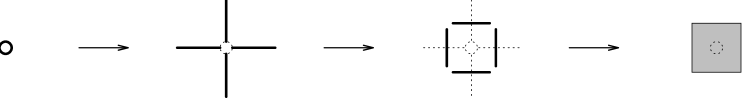
Figure 1: Lattice transformations (only one site shown)

We start with the Ashkin–Teller model in $\Lambda$ with $(+,+)$-boundary condition. Let us consider some site $t\in\Lambda$. We then define the corresponding GRC model with $(+,+)$-boundary condition: here the bonds whose value is not fixed are all bonds whose boundary contains at least one site of $\Lambda$ (among them, there are in particular the four bonds with an endpoint at $t$). Then we take its dual model with free boundary condition: now, the bonds whose value is not fixed are the dual bonds crossing the previous ones. But the four dual bonds around $t$ are the boundary of a plaquette $p^{*}$ having $t$ as its center (see fig 1). Hence, to each $t\in\Lambda$, this associates a plaquette $p^{*}(t)$ having $t$ as its center: this is just the definition we have given of $\Lambda^{*}$. Therefore these four bonds belong to ${\cal B}(\Lambda^{*})$. Doing this for all sites of $\Lambda$, we obtain all of ${\cal B}(\Lambda^{*})$.

Using the preceding geometrical results, we can write

$$\sum_{+,\Lambda}f({\underline{n}})\lambda_{{\cal B}^{+}(\Lambda)}({\underline{n}})q_{\sigma}^{{N_{\sigma}}({\underline{n}}|\Lambda)}q_{\tau}^{{N_{\tau}}({\underline{n}}|\Lambda)}=$$

$$\;\;=\sum_{{\underline{n}}:\atop(+,+)\mbox{\tiny-b.c. in }\Lambda}f({\underline{n}})\cdot\biggl{(}\prod_{\scriptstyle b\in{\cal B}^{+}(\Lambda):\atop\scriptstyle n_{b}=(0,0)}a_{0}(b)\prod_{\scriptstyle b\in{\cal B}^{+}(\Lambda):\atop\scriptstyle n_{b}=(1,0)}a_{\sigma}(b)\prod_{\scriptstyle b\in{\cal B}^{+}(\Lambda):\atop\scriptstyle n_{b}=(0,1)}a_{\tau}(b)\prod_{\scriptstyle b\in{\cal B}^{+}(\Lambda):\atop\scriptstyle n_{b}=(1,1)}a_{\sigma\tau}(b)\biggr{)}\times$$

$$\;\;\;\;\;\times q_{\sigma}^{{N_{\sigma}}({\underline{n}}|\Lambda)}q_{\tau}^{{N_{\tau}}({\underline{n}}|\Lambda)}$$

$$\;\;=C\sum_{\hat{\underline{n}}:\atop\mbox{\tiny free b.c. in }\Lambda^{*}}f({\underline{n}})\cdot\biggl{(}\prod_{\scriptstyle{\hat{b}}\in{\cal B}(\Lambda^{*}):\atop\scriptstyle\hat{n}_{\hat{b}}=(1,1)}a_{0}(b)\prod_{\scriptstyle{\hat{b}}\in{\cal B}(\Lambda^{*}):\atop\scriptstyle\hat{n}_{\hat{b}}=(1,0)}a_{\sigma}(b)\prod_{\scriptstyle{\hat{b}}\in{\cal B}(\Lambda^{*}):\atop\scriptstyle\hat{n}_{\hat{b}}=(0,1)}a_{\tau}(b)\prod_{\scriptstyle{\hat{b}}\in{\cal B}(\Lambda^{*}):\atop\scriptstyle\hat{n}_{\hat{b}}=(0,0)}a_{\sigma\tau}(b)\biggr{)}\times$$

$$\;\;\;\;\;\times q_{\sigma}^{{N_{\tau}}(\hat{\underline{n}}|\Lambda)+|\hat{\underline{n}}_{\tau}|}q_{\tau}^{{N_{\sigma}}(\hat{\underline{n}}|\Lambda)+|\hat{\underline{n}}_{\sigma}|}$$

$$\;\;=C\sum_{\hat{\underline{n}}:\atop\mbox{\tiny free b.c. in }\Lambda^{*}}f({\underline{n}})\cdot\biggl{(}\prod_{\scriptstyle{\hat{b}}\in{\cal B}(\Lambda^{*}):\atop\scriptstyle\hat{n}_{\hat{b}}=(1,1)}\hat{a}_{\sigma\tau}({\hat{b}})\prod_{\scriptstyle{\hat{b}}\in{\cal B}(\Lambda^{*}):\atop\scriptstyle\hat{n}_{\hat{b}}=(1,0)}\hat{a}_{\sigma}({\hat{b}})\prod_{\scriptstyle{\hat{b}}\in{\cal B}(\Lambda^{*}):\atop\scriptstyle\hat{n}_{\hat{b}}=(0,1)}\hat{a}_{\tau}({\hat{b}})\prod_{\scriptstyle{\hat{b}}\in{\cal B}(\Lambda^{*}):\atop\scriptstyle\hat{n}_{\hat{b}}=(0,0)}\hat{a}_{0}({\hat{b}})\biggr{)}\times$$

$$\;\;\;\;\;\times\widehat{q}_{\sigma}^{{N_{\sigma}}(\hat{\underline{n}}|\Lambda)}\widehat{q}_{\tau}^{{N_{\tau}}(\hat{\underline{n}}|\Lambda)}\,,$$ (3.32)

where $C$ denote some constant independent on ${\underline{n}}$, $|\hat{\underline{n}}|$ is the number of open bonds in $\hat{\underline{n}}$ and we have introduced

$$\hat{a}_{0}({\hat{b}}) := C^{\prime}a_{\sigma\tau}(b)\,,$$

$$\hat{a}_{\sigma}({\hat{b}}) := q_{\tau}C^{\prime}a_{\sigma}(b)\,,$$

$$\hat{a}_{\tau}({\hat{b}}) := q_{\sigma}C^{\prime}a_{\tau}(b)\,,$$

$$\hat{a}_{\sigma\tau}({\hat{b}}) := q_{\sigma}q_{\tau}C^{\prime}a_{0}(b)\,,$$

$$\widehat{q}_{\sigma} := q_{\tau}\,,$$

$$\widehat{q}_{\tau} := q_{\sigma}\,.$$ (3.33)

$C^{\prime}$ is a normalization constant such that $\hat{a}_{0}+\hat{a}_{\sigma}+\hat{a}_{\tau}+\hat{a}_{\sigma\tau}=1$:

$$C^{\prime-1}=a_{\sigma\tau}+q_{\tau}a_{\sigma}+q_{\sigma}a_{\tau}+q_{\sigma}q_{\tau}a_{0}\,.$$ (3.34)

Remark: 1) Note that the positivity of theses dual probabilities is a consequence of the
positivity of the initial probabilities.
	2) There are no other way to distribute the factors $q_{\sigma}$ and $q_{\tau}$ in (3.32).

As a consequence we have

Proposition 3.2

Let $\Lambda$ be a finite, simply connected subset of ${\mathchoice{\hbox{$\sf\textstyle Z\kern-3.99994ptZ$}}{\hbox{$\sf\textstyle Z\kern-3.99994ptZ$}}{\hbox{$\sf\scriptstyle Z\kern-2.10002ptZ$}}{\hbox{$\sf\scriptscriptstyle Z\kern-0.99998ptZ$}}}^{2}$. Let $\hat{a}_{0}$, $\hat{a}_{\sigma}$, $\hat{a}_{\tau}$ and $\hat{a}_{\sigma\tau}$ be defined by (3.4). Then, for all $f\in{\cal F}^{2}$,

$$\nu_{\Lambda}^{+}(f|a_{0},a_{\sigma},a_{\tau},a_{\sigma\tau},q_{\sigma},q_{\tau})=\nu^{f}_{\Lambda^{*}}(\widehat{f}|\hat{a}_{0},\hat{a}_{\sigma},\hat{a}_{\tau},\hat{a}_{\sigma\tau},\hat{q}_{\sigma},\hat{q}_{\tau})\,,$$ (3.35)

where $\widehat{f}(\hat{\underline{n}}):=f({\underline{n}}(\hat{\underline{n}}))$.

A natural question to ask is: do the transformations between the spin and random–cluster models and the duality transformations commute in the Ashkin–Teller case? The answer is yes, as is shown below.

3.5 Commutativity of the dualities and RC transformation

We want to compare the dual of the generalized random–cluster model associated to the Ashkin–Teller model with $(+,+)$-boundary conditions with the random–cluster model associated to the dual of this Ashkin–Teller model.

For the dual of the random–cluster model, we obtain (see (3.4) and (3.14))

$$\hat{a}_{0} = \frac{1-j_{\sigma\tau}(j_{\sigma}+j_{\tau})+j_{\sigma}j_{\tau}}{1+j_{\sigma\tau}(j_{\sigma}+j_{\tau})+j_{\sigma}j_{\tau}}\,,$$

$$\hat{a}_{\sigma} = \frac{2j_{\tau}(j_{\sigma\tau}-j_{\sigma})}{1+j_{\sigma\tau}(j_{\sigma}+j_{\tau})+j_{\sigma}j_{\tau}}\,,$$

$$\hat{a}_{\tau} = \frac{2j_{\sigma}(j_{\sigma\tau}-j_{\tau})}{1+j_{\sigma\tau}(j_{\sigma}+j_{\tau})+j_{\sigma}j_{\tau}}\,,$$

$$\hat{a}_{\sigma\tau} = 1-\hat{a}_{0}-\hat{a}_{\sigma}-\hat{a}_{\tau}\,,$$ (3.36)

where $j_{\sigma}=\mathchoice{\mbox{$\displaystyle\rm e$}}{\mbox{$\textstyle\rm e$}}{\mbox{$\scriptstyle\rm e$}}{\mbox{$\scriptscriptstyle\rm e$}}^{-2J_{\sigma}}$, $j_{\tau}=\mathchoice{\mbox{$\displaystyle\rm e$}}{\mbox{$\textstyle\rm e$}}{\mbox{$\scriptstyle\rm e$}}{\mbox{$\scriptscriptstyle\rm e$}}^{-2J_{\tau}}$, $j_{\sigma\tau}=\mathchoice{\mbox{$\displaystyle\rm e$}}{\mbox{$\textstyle\rm e$}}{\mbox{$\scriptstyle\rm e$}}{\mbox{$\scriptscriptstyle\rm e$}}^{-2J_{\sigma\tau}}$.

For the random–cluster of the dual model, we find (see (2.11) and (3.14))

$$a_{0}^{*} = \frac{l+st}{1+stl}\,,$$

$$a_{\sigma}^{*} = \frac{(t-l)(1-s)}{1+stl}\,,$$

$$a_{\tau}^{*} = \frac{(s-l)(1-t)}{1+stl}\,,$$

$$a_{\sigma\tau}^{*} = 1-a_{0}^{*}-a_{\sigma}^{*}-a_{\tau}^{*}\,.$$ (3.37)

where $l$, $s$, $t$ have been defined in (2.6). Using the relations:

$$s=\frac{1-j_{\sigma}}{1+j_{\sigma}},\phantom{m}t=\frac{1-j_{\tau}}{1+j_{\tau}},\phantom{m}l=\frac{1-j_{\sigma\tau}}{1+j_{\sigma\tau}}\,,$$

it is easy to see that the quantities defined in (3.36) and (3.37) are in fact the same.

We have already checked that both resulting models are defined on the same lattice (see section 3.4), so we can conclude that the following diagram is commutative:

Here ${\cal F}{\cal K}$ denotes the random–cluster transformation and * the dualities.

We now turn to the properties of the generalized random–cluster model.

4 Properties of the GRC measure

4.1 FKG inequalities

In this section we are going to show that the measures of the generalized random–cluster model which have been introduced are FKG. No hypothesis on $\Lambda$, except its boundedness, is required.

We partition the bonds into two classes:

$${{\cal B}}_{>}=\{b:a_{\sigma\tau}(b)a_{0}(b)\geq a_{\sigma}(b)a_{\tau}(b)\}\,,$$

$${{\cal B}}_{<}=\{b:a_{\sigma\tau}(b)a_{0}(b)<a_{\sigma}(b)a_{\tau}(b)\}\,.$$ (4.1)

We introduce the following partial order on $\{0,1\}\times\{0,1\}$:

$$(0,0)\preceq(0,1)\preceq(1,1),\phantom{m}\phantom{m}(0,0)\preceq(1,0)\preceq(1,1)\,,$$ (4.2)

for bonds in ${\cal B}_{>}$, and

$$(0,1)\preceq(1,1)\preceq(1,0),\phantom{m}\phantom{m}(0,1)\preceq(0,0)\preceq(1,0)\,,$$ (4.3)

for bonds in ${\cal B}_{<}$.

For the generalized random–cluster associated to the Ashkin–Teller model, it is easy to see that all bonds will be in ${\cal B}_{>}$ if $J_{\sigma\tau}\geq 0$ and in ${\cal B}_{<}$ if $J_{\sigma\tau}<0$.

Definition 4.1

Let $\underline{m}$ and $\underline{n}$ be two configurations. $\underline{m}$ is said to dominate $\underline{n}$, $\underline{m}\succeq\underline{n}$, if $m_{b}\succeq n_{b}$, $\forall b$.

Definition 4.2

A function f is said to be increasing if $\underline{m}\succeq\underline{n}\Rightarrow f(\underline{m})\geq f(\underline{n})$. It is said to be decreasing if $-f$ is increasing.

Example:$\,{N_{\sigma}}({\underline{n}}|\Lambda)$ and ${N_{\tau}}({\underline{n}}|\Lambda)+\sum_{b\in{\cal B}_{<}}n_{\tau,b}$ are decreasing functions for the order defined above, while ${N_{\sigma}}({\underline{n}}|\Lambda)+\sum_{b}n_{\sigma,b}$ and ${N_{\tau}}({\underline{n}}|\Lambda)+\sum_{b\in{\cal B}_{>}}n_{\tau,b}$ are increasing functions.
Let us just look at the case ${N_{\tau}}({\underline{n}}|\Lambda)+\sum_{b\in{\cal B}_{>}}n_{\tau,b}$. It is sufficient to consider two configurations ${\underline{n}}\succeq\hat{\underline{n}}$, differing only by one $\tau$-bond at $b$.
There are two cases: either $b\in{\cal B}_{>}$, or $b\in{\cal B}_{<}$. In the first case the $\tau$-bond is missing in $\hat{\underline{n}}$ and hence we have

$${N_{\tau}}(\hat{\underline{n}}|\Lambda)+\sum_{b\in{\cal B}_{>}}\hat{n}_{\tau,b}={N_{\tau}}({\underline{n}}|\Lambda)+\sum_{b\in{\cal B}_{>}}n_{\tau,b}+({N_{\tau}}(\hat{\underline{n}}|\Lambda)-{N_{\tau}}({\underline{n}}|\Lambda))-1\leq{N_{\tau}}({\underline{n}}|\Lambda)+\sum_{b\in{\cal B}_{>}}n_{\tau,b}\,,$$

since $|{N_{\tau}}(\hat{\underline{n}}|\Lambda)-{N_{\tau}}({\underline{n}}|\Lambda)|\leq 1$.
If $b\in{\cal B}_{<}$, then the bond is missing in ${\underline{n}}$ and

$${N_{\tau}}(\hat{\underline{n}}|\Lambda)+\sum_{b\in{\cal B}_{>}}\hat{n}_{\tau,b}={N_{\tau}}({\underline{n}}|\Lambda)+\sum_{b\in{\cal B}_{>}}n_{\tau,b}+({N_{\tau}}(\hat{\underline{n}}|\Lambda)-{N_{\tau}}({\underline{n}}|\Lambda))\leq{N_{\tau}}({\underline{n}}|\Lambda)+\sum_{b\in{\cal B}_{>}}n_{\tau,b}\,.$$

Indeed, the $\tau$-bond links two sites already in the same $\tau$-cluster and therefore the number of such clusters doesn’t change, or it links two different clusters and ${N_{\tau}}(\hat{\underline{n}}|\Lambda)-{N_{\tau}}({\underline{n}}|\Lambda)=-1$.

Definition 4.3

A measure $\mu$ is said to be FKG if $\mu(fg)\geq\mu(f)\mu(g)$, for all increasing functions $f$ and $g$.

Lemma 4.1

The generalized percolation measure $\lambda_{\cal B}$ is FKG for the partial order introduced above.

Proof. It is sufficient to check that (see [FKG])

$$\lambda_{\cal B}({\underline{n}}\vee{\underline{n}}^{\prime})\lambda_{\cal B}({\underline{n}}\wedge{\underline{n}}^{\prime})\geq\lambda_{\cal B}({\underline{n}})\lambda_{\cal B}({\underline{n}}^{\prime})\,,$$

where $a\vee b$ denotes the least upper bound of $a$ and $b$, while $a\wedge b$ denotes their greatest lower bound. As $\lambda_{\cal B}$ is a product-measure, it is sufficient to verify this for each bond, which is straightforward. The only non-trivial inequalities are:

$$\lambda_{b}((1,1))\lambda_{b}((0,0))\geq\lambda_{b}((1,0))\lambda_{b}((0,1))\,,$$

for bonds in ${\cal B}_{>}$, but this is satisfied by definition of this class of bonds; and

$$\lambda_{b}((1,0))\lambda_{b}((0,1))\geq\lambda_{b}((1,1))\lambda_{b}((0,0))\,,$$

for bonds in ${\cal B}_{<}$, which is also true by definition. $\sqcap$$\sqcup$

Proposition 4.1

Suppose $q_{\sigma}\geq 1$ and $q_{\tau}\geq 1$. Then the random–cluster measure is FKG for the partial order introduced above.

Proof. It is sufficient to check (see [FKG]) that

$$q_{\sigma}^{{N_{\sigma}}({\underline{n}}\vee{\underline{n}}^{\prime}|\Lambda)+{N_{\sigma}}({\underline{n}}\wedge{\underline{n}}^{\prime}|\Lambda)}q_{\tau}^{{N_{\tau}}({\underline{n}}\vee{\underline{n}}^{\prime}|\Lambda)+{N_{\tau}}({\underline{n}}\wedge{\underline{n}}^{\prime}|\Lambda)}\geq q_{\sigma}^{{N_{\sigma}}({\underline{n}}|\Lambda)+{N_{\sigma}}({\underline{n}}^{\prime}|\Lambda)}q_{\tau}^{{N_{\tau}}({\underline{n}}|\Lambda)+{N_{\tau}}({\underline{n}}^{\prime}|\Lambda)}\,,$$

which can be proved exactly as in the case of the usual random–cluster model [ACCN]. The only thing to observe is that

$${N_{\sigma}}({\underline{n}}{\vee}{\underline{n}}^{\prime}|\Lambda) = {N_{\sigma}}({\underline{n}}\widehat{\vee}{\underline{n}}^{\prime}|\Lambda)\,,$$

$${N_{\sigma}}({\underline{n}}{\wedge}{\underline{n}}^{\prime}|\Lambda) = {N_{\sigma}}({\underline{n}}\widehat{\wedge}{\underline{n}}^{\prime}|\Lambda)\,,$$

$${N_{\tau}}({\underline{n}}{\wedge}{\underline{n}}^{\prime}|\Lambda) = {N_{\tau}}({\underline{n}}\widehat{\vee}{\underline{n}}^{\prime}|\Lambda)\,,$$

$${N_{\tau}}({\underline{n}}{\vee}{\underline{n}}^{\prime}|\Lambda) = {N_{\tau}}({\underline{n}}\widehat{\wedge}{\underline{n}}^{\prime}|\Lambda)\,,$$

where $\widehat{\vee}$ and $\widehat{\wedge}$ denote the order induced by setting the order (4.2) at all bonds. Hence,

$${N_{\sigma}}({\underline{n}}{\vee}{\underline{n}}^{\prime}|\Lambda)+{N_{\sigma}}({\underline{n}}{\wedge}{\underline{n}}^{\prime}|\Lambda) = {N_{\sigma}}({\underline{n}}\widehat{\vee}{\underline{n}}^{\prime}|\Lambda)+{N_{\sigma}}({\underline{n}}\widehat{\wedge}{\underline{n}}^{\prime}|\Lambda)\,,$$

$${N_{\tau}}({\underline{n}}{\vee}{\underline{n}}^{\prime}|\Lambda)+{N_{\tau}}({\underline{n}}{\wedge}{\underline{n}}^{\prime}|\Lambda) = {N_{\tau}}({\underline{n}}\widehat{\vee}{\underline{n}}^{\prime}|\Lambda)+{N_{\tau}}({\underline{n}}\widehat{\wedge}{\underline{n}}^{\prime}|\Lambda)\,.$$

$\sqcap$$\sqcup$

As direct elementary applications of these inequalities to the Ashkin–Teller model, we have

$$\mu_{\Lambda}^{\circ}(\sigma_{i}\sigma_{j})=\nu_{\Lambda}^{\bullet}(i\mathop{\leftrightarrow}^{\sigma}j) \geq \nu_{\Lambda}^{\bullet}(i\mathop{\leftrightarrow}^{\sigma}\Lambda^{c}\mbox{ and }j\mathop{\leftrightarrow}^{\sigma}\Lambda^{c})$$ (4.5)

$$\geq \nu_{\Lambda}^{\bullet}(i\mathop{\leftrightarrow}^{\sigma}\Lambda^{c})\nu_{\Lambda}^{\bullet}(j\mathop{\leftrightarrow}^{\sigma}\Lambda^{c})=\mu_{\Lambda}^{\circ}(\sigma_{i})\mu_{\Lambda}^{\circ}(\sigma_{j})\,,$$

which is nothing more than one of Griffith’s inequalities. Here $\circ$ means any boundary conditions for the Ashkin–Teller model and $\bullet$ the corresponding boundary conditions for the random–cluster model.

More interesting is the following inequality, which holds in the case $J_{\sigma\tau}\leq 0$ (for which we cannot use Griffith’s inequalities),

$$\mu_{\Lambda}^{++}(\sigma_{i}\sigma_{j}\tau_{k}\tau_{l})=\nu_{\Lambda}^{+}(i\mathop{\leftrightarrow}^{\sigma}j,k\mathop{\leftrightarrow}^{\tau}l)\leq\nu_{\Lambda}^{+}(i\mathop{\leftrightarrow}^{\sigma}j)\nu_{\Lambda}^{+}(k\mathop{\leftrightarrow}^{\tau}l)=\mu_{\Lambda}^{++}(\sigma_{i}\sigma_{j})\mu_{\Lambda}^{++}(\tau_{k}\tau_{l})\,,$$

where we have used the fact that $\displaystyle k\mathop{\leftrightarrow}^{\tau}l$ is decreasing for the order $\preceq$.
More generally, we have, for negative $J_{\sigma\tau}$,

$$\mu_{\Lambda}(\sigma_{A}\sigma_{B}) \geq \mu_{\Lambda}(\sigma_{A})\mu_{\Lambda}(\sigma_{B})\,,$$

$$\mu_{\Lambda}(\tau_{A}\tau_{B}) \geq \mu_{\Lambda}(\tau_{A})\mu_{\Lambda}(\tau_{B})\,,$$

$$\mu_{\Lambda}(\sigma_{A}\tau_{B}) \leq \mu_{\Lambda}(\sigma_{A})\mu_{\Lambda}(\tau_{B})\,,$$

as can be easily verified (this is true for free, as well as for $(+,+)$-boundary conditions).

4.2 Comparison inequalities

There is a class of inequalities in the usual random–cluster model which is very interesting: they allow one to compare the probability of an event for different values of $q$ and of the probability of occupation. It is possible to generalize these inequalities here, as shown now.

We consider two random–cluster measures, $\nu_{\Lambda}$ and $\widehat{\nu}_{\Lambda}$, with parameters $a_{0}$, $a_{\sigma}$, $a_{\tau}$, $a_{\sigma\tau}$, $q_{\sigma}$, $q_{\tau}$ and $\hat{a}_{0}$, $\hat{a}_{\sigma}$, $\hat{a}_{\tau}$, $\hat{a}_{\sigma\tau}$, $\hat{q}_{\sigma}$, $\hat{q}_{\tau}$, respectively. What is the relation between the probabilities of monotonous events computed with these two measures? We will consider only two cases, but others can be proved in the same way.

We introduce the following notations

$$\displaystyle\rho_{\sigma}=\frac{q_{\sigma}}{\hat{q}_{\sigma}},\;\displaystyle\rho_{\tau}=\frac{q_{\tau}}{\hat{q}_{\tau}},$$ (4.6)

$$\displaystyle\alpha_{0}=\frac{a_{0}}{\hat{a}_{0}},\;\displaystyle\alpha_{\sigma}=\frac{a_{\sigma}}{\hat{a}_{\sigma}},\;\displaystyle\alpha_{\tau}=\frac{a_{\tau}}{\hat{a}_{\tau}},\;\displaystyle\alpha_{\sigma\tau}=\frac{a_{\sigma\tau}}{\hat{a}_{\sigma\tau}}.$$ (4.7)

We can now formulate our first inequality.

Lemma 4.2

Suppose $\hat{q}_{\sigma}$, $\hat{q}_{\tau}\geq 1$, and

$$q_{\sigma}\leq\hat{q}_{\sigma}\,,\;q_{\tau}\leq\hat{q}_{\tau}\,,$$ (4.8)

$$\displaystyle\alpha_{\sigma\tau}\geq\max(\alpha_{\sigma},\alpha_{\tau})\geq\min(\alpha_{\sigma},\alpha_{\tau})\geq\alpha_{0},\forall b\in{\cal B}_{>}\,,$$ (4.9)

$$\displaystyle\rho_{\tau}\alpha_{\sigma}\geq\max(\alpha_{\sigma\tau},\rho_{\tau}\alpha_{0})\geq\min(\alpha_{\sigma\tau},\rho_{\tau}\alpha_{0})\geq\alpha_{\tau}\,,\;\forall b\in{\cal B}_{<}\,,$$ (4.10)

then, for every increasing function $A$,

$$\nu_{\Lambda}(A)\geq\widehat{\nu}_{\Lambda}(A)\,.$$

Proof. Let $\chi({\underline{n}})=\frac{\nu_{\Lambda}({\underline{n}})}{\widehat{\nu}_{\Lambda}({\underline{n}})}$. We are going to write $\chi$ in such a way as to make explicit the monotonicity of this function under the above hypotheses.

$$\chi = C\left\{\prod_{b\in{\cal B}_{>}}\left(\frac{a_{0}}{\hat{a}_{0}}\right)^{{\overline{n}}_{\sigma,b}{\overline{n}}_{\tau,b}}\left(\frac{a_{\sigma}}{\hat{a}_{\sigma}}\right)^{n_{\sigma,b}{\overline{n}}_{\tau,b}}\left(\frac{a_{\tau}}{\hat{a}_{\tau}}\right)^{{\overline{n}}_{\sigma,b}n_{\tau,b}}\left(\frac{a_{\sigma\tau}}{\hat{a}_{\sigma\tau}}\right)^{n_{\sigma,b}n_{\tau,b}}\right\}\times$$

$$\times\left\{\prod_{b\in{\cal B}_{<}}\left(\frac{q_{\tau}}{\hat{q}_{\tau}}\frac{a_{0}}{\hat{a}_{0}}\right)^{{\overline{n}}_{\sigma,b}{\overline{n}}_{\tau,b}}\left(\frac{q_{\tau}}{\hat{q}_{\tau}}\frac{a_{\sigma}}{\hat{a}_{\sigma}}\right)^{n_{\sigma,b}{\overline{n}}_{\tau,b}}\left(\frac{a_{\tau}}{\hat{a}_{\tau}}\right)^{{\overline{n}}_{\sigma,b}n_{\tau,b}}\left(\frac{a_{\sigma\tau}}{\hat{a}_{\sigma\tau}}\right)^{n_{\sigma,b}n_{\tau,b}}\right\}\times$$

$$\times\left(\frac{q_{\sigma}}{\hat{q}_{\sigma}}\right)^{{N_{\sigma}}({\underline{n}}|\Lambda)}\left(\frac{q_{\tau}}{\hat{q}_{\tau}}\right)^{{N_{\tau}}({\underline{n}}|\Lambda)+\sum_{b\in{\cal B}_{<}}n_{\tau,b}}\,,$$

where $C>0$ is a constant independent on the configuration.
Now, using (4.8) and the fact that ${N_{\sigma}}({\underline{n}}|\Lambda)$ and ${N_{\tau}}({\underline{n}}|\Lambda)+\sum_{b\in{\cal B}_{<}}n_{\tau,b}$ are decreasing, it is easy to see that $\chi$ will be increasing if what is inside the brackets is increasing; and this will be true if it is true for each bond. This can be easily checked. We just consider two examples, since the other cases can be treated in the same way.
Let us first verify that the expression in the first brackets is not decreasing when $n_{b}$ increases from $(1,0)$ to $(1,1)$. In the first case this expression equals ${a_{\sigma}}/{\hat{a}_{\sigma}}$, while in the second it equals $a_{\sigma\tau}/{\hat{a}_{\sigma\tau}}$, which is not smaller by hypothesis.
Let’s now show that the expression in the second brackets does not decrease when $n_{b}$ increases from $(1,1)$ to $(1,0)$. But this amounts to $a_{\sigma\tau}/{\hat{a}_{\sigma\tau}}\leq{q_{\tau}a_{\sigma}}/{\hat{q}_{\tau}\hat{a}_{\sigma}}$ which is true by hypothesis.
Doing the same computation for the other cases, we finally obtain

$$\nu_{\Lambda}(A)=\widehat{\nu}_{\Lambda}(A|\chi)\geq\widehat{\nu}_{\Lambda}(A)\,,$$

by FKG and the fact that $\widehat{\nu}_{\Lambda}$ and $\nu_{\Lambda}$ are normalized.

$\sqcap$$\sqcup$We now give a second inequality,

Lemma 4.3

Suppose $\hat{q}_{\sigma}$, $\hat{q}_{\tau}\geq 1$, and

$$q_{\sigma}\geq\hat{q}_{\sigma}\,,\;q_{\tau}\geq\hat{q}_{\tau}\,,$$ (4.11)

$$\displaystyle\alpha_{\sigma\tau}\geq\max(\rho_{\tau}\alpha_{\sigma},\rho_{\sigma}\alpha_{\tau})\geq\min(\rho_{\tau}\alpha_{\sigma},\rho_{\sigma}\alpha_{\tau})\geq\rho_{\sigma}\rho_{\tau}\alpha_{0}\,,\;\forall b\in{\cal B}_{>}\,,$$ (4.12)

$$\displaystyle\alpha_{\sigma}\geq\max(\alpha_{\sigma\tau},\rho_{\sigma}\alpha_{0})\geq\min(\alpha_{\sigma\tau},\rho_{\sigma}\alpha_{0})\geq\rho_{\sigma}\alpha_{\tau},\forall b\in{\cal B}_{<}\,,$$ (4.13)

then, for every increasing function $A$,

$$\nu_{\Lambda}(A)\geq\widehat{\nu}_{\Lambda}(A)\,.$$

Proof. As above, using the fact that ${N_{\sigma}}({\underline{n}}|\Lambda)+|{\underline{n}}_{\sigma}|$ and ${N_{\tau}}({\underline{n}}|\Lambda)+\sum_{b\in{\cal B}_{>}}n_{\tau,b}$ are increasing. $\sqcap$$\sqcup$

Remark: As said before, other such inequalities can be proved in exactly the same way, for example when $q_{\sigma}$ increases but $q_{\tau}$ decreases.

As a simple application of these inequalities, we prove inequalities relating the generalized random–cluster model to the usual one.

Lemma 4.4

Suppose $q_{\sigma}$, $q_{\tau}\geq 1$, $f\in{\cal F}_{\sigma}$, increasing, then

$$\rho_{\Lambda}(f_{\sigma}|p_{1},q_{\sigma})\leq\nu_{\Lambda}(f|q_{\sigma},q_{\tau})\leq\rho_{\Lambda}(f_{\sigma}|p_{2},q_{\sigma})\,,$$

where

$$p_{1}=\frac{q_{\tau}a_{\sigma}+a_{\sigma\tau}}{q_{\tau}(a_{0}+a_{\sigma})+a_{\tau}+a_{\sigma\tau}}\,,$$

$$p_{2}=a_{\sigma}+a_{\sigma\tau}\,.$$

The same kind of relations holds for $f\in{\cal F}_{\tau}$.

Proof.

$$\nu_{\Lambda}(f|q_{\sigma},q_{\tau})\leq\nu_{\Lambda}(f|q_{\sigma},1)=\rho_{\Lambda}(f_{\sigma}|p=a_{\sigma}+a_{\sigma\tau},q_{\sigma})\,,$$

where we used lemma 4.2 and lemma 3.2. In a similar way,

$$\nu_{\Lambda}(f|q_{\sigma},q_{\tau}) \geq \nu_{\Lambda}(f|q_{\sigma},q_{\tau}=1,\hat{a}_{0}=\frac{q_{\tau}a_{0}}{N},\hat{a}_{\sigma}=\frac{q_{\tau}a_{\sigma}}{N},\hat{a}_{\tau}=\frac{a_{\tau}}{N},\hat{a}_{\sigma\tau}=\frac{a_{\sigma\tau}}{N})$$

$$= \rho_{\Lambda}(f_{\sigma}|(q_{\tau}a_{\sigma}+a_{\sigma\tau})/(q_{\tau}(a_{0}+a_{\sigma})+a_{\tau}+a_{\sigma\tau}),q_{\sigma})\,,$$

where $N=q_{\tau}(a_{0}+a_{\sigma})+a_{\tau}+a_{\sigma\tau}$ is the normalization of the new probabilities, and we used lemma 4.3 and lemma 3.2. $\sqcap$$\sqcup$

From this lemma we can for example obtain estimates on the location of the critical lines of the Ashkin–Teller model in the sector $J_{\sigma\tau}\geq J_{\sigma}=J_{\tau}=:J\geq 0$, in which the critical line splits into two parts, the first one corresponding to the ordering of the $\sigma_{i}$ and $\tau_{i}$, and the other one to the ordering of the $\theta_{i}=\sigma_{i}\tau_{i}$ (see fig. 2). Let’s study this second line.

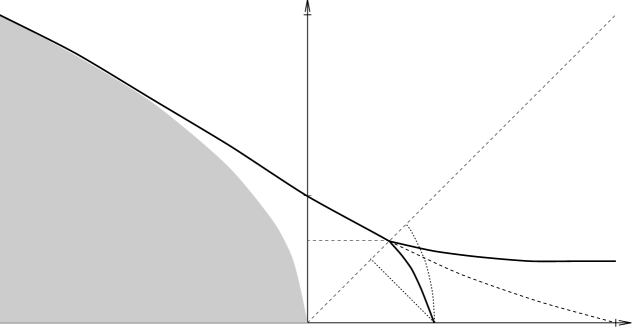
Figure 2: Schematic representation of the phase diagram in the plane $\tanh J_{\sigma\tau}$ versus $\tanh J_{\sigma}=\tanh J_{\tau}$. We have indicated the critical lines (solid lines), and the self–dual line (which coincides with the solid line up to the splitting and then follows the dashed line). The shaded region corresponds to the set of parameters at which the random–cluster representation is not available. The estimates of the location of the critical line are also shown (dotted lines).

We first make the change of variables $(\sigma,\tau)\mapsto(\theta,\tau)$. The previous lemma then gives, specializing to the increasing event $\{i\mathop{\leftrightarrow}^{\theta}\Lambda^{c}\}$,

$$\rho_{\Lambda}(i\mathop{\leftrightarrow}^{\theta}\Lambda^{c}|(2a_{\theta}+a_{\theta\tau})/(1+a_{0}+a_{\theta}),2)\leq\nu_{\Lambda}(i\mathop{\leftrightarrow}^{\theta}\Lambda^{c}|2,2)\leq\rho_{\Lambda}(i\mathop{\leftrightarrow}^{\theta}\Lambda^{c}|a_{\theta}+a_{\theta\tau},2)\,,$$

which can be rewritten in terms of the original Ashkin–Teller and Ising measures:

$$\eta_{\Lambda}(\theta_{i}|J_{1})\leq\mu_{\Lambda}(\theta_{i})\leq\eta_{\Lambda}(\theta_{i}|J_{2})\,,$$ (4.14)

where $\eta_{\Lambda}(\cdot|J)$ denotes the Ising measure with coupling constant $J$, and the coupling constants $J_{1}$ and $J_{2}$ are given by

$$J_{1} = J_{\sigma\tau}+\frac{1}{2}\ln\mathchoice{\mbox{$\displaystyle\rm cosh$}}{\mbox{$\textstyle\rm cosh$}}{\mbox{$\scriptstyle\rm cosh$}}{\mbox{$\scriptscriptstyle\rm cosh$}}(2J)\,,$$

$$J_{2} = J+J_{\sigma\tau}\,.$$

The upper bound in (4.14) is easily obtained using GKS inequalities. This seems not to be the case for the lower bound.

Since we know the critical temperature of these two Ising models, we obtain the following results (remember $\theta_{i}=\sigma_{i}\tau_{i}$):

$$J_{\sigma\tau}\leq J^{c}_{\mathchoice{\mbox{$\displaystyle\rm Ising$}}{\mbox{$\textstyle\rm Ising$}}{\mbox{$\scriptstyle\rm Ising$}}{\mbox{$\scriptscriptstyle\rm Ising$}}}-J\Rightarrow\mu(\sigma\tau)=0\,,$$ (4.15)

$$J_{\sigma\tau}>J^{c}_{\mathchoice{\mbox{$\displaystyle\rm Ising$}}{\mbox{$\textstyle\rm Ising$}}{\mbox{$\scriptstyle\rm Ising$}}{\mbox{$\scriptscriptstyle\rm Ising$}}}-\frac{1}{2}\ln\mathchoice{\mbox{$\displaystyle\rm cosh$}}{\mbox{$\textstyle\rm cosh$}}{\mbox{$\scriptstyle\rm cosh$}}{\mbox{$\scriptscriptstyle\rm cosh$}}(2J)\Rightarrow\mu(\sigma\tau)>0\,,$$ (4.16)

where $J^{c}_{\mathchoice{\mbox{$\displaystyle\rm Ising$}}{\mbox{$\textstyle\rm Ising$}}{\mbox{$\scriptstyle\rm Ising$}}{\mbox{$\scriptscriptstyle\rm Ising$}}}=\frac{1}{2}\mathchoice{\mbox{$\displaystyle\rm\mathchoice{\mbox{$\displaystyle\rm argsinh$}}{\mbox{$\textstyle\rm argsinh$}}{\mbox{$\scriptstyle\rm argsinh$}}{\mbox{$\scriptscriptstyle\rm argsinh$}}$}}{\mbox{$\textstyle\rm\mathchoice{\mbox{$\displaystyle\rm argsinh$}}{\mbox{$\textstyle\rm argsinh$}}{\mbox{$\scriptstyle\rm argsinh$}}{\mbox{$\scriptscriptstyle\rm argsinh$}}$}}{\mbox{$\scriptstyle\rm\mathchoice{\mbox{$\displaystyle\rm argsinh$}}{\mbox{$\textstyle\rm argsinh$}}{\mbox{$\scriptstyle\rm argsinh$}}{\mbox{$\scriptscriptstyle\rm argsinh$}}$}}{\mbox{$\scriptscriptstyle\rm\mathchoice{\mbox{$\displaystyle\rm argsinh$}}{\mbox{$\textstyle\rm argsinh$}}{\mbox{$\scriptstyle\rm argsinh$}}{\mbox{$\scriptscriptstyle\rm argsinh$}}$}}1$ is Ising critical temperature.

Remark: Such a behaviour cannot occur in the sector $J_{\sigma}=J_{\tau}\geq J_{\sigma\tau}\geq 0$. Indeed, in this case,

$$\mu_{\Lambda}(\sigma_{i}) = \nu_{\Lambda}(i\mathop{\leftrightarrow}^{\sigma}\Lambda^{c})\geq\nu_{\Lambda}(i\mathop{\leftrightarrow}^{\sigma}\Lambda^{c}\mbox{ and }{i\mathop{\leftrightarrow}^{\tau}\Lambda^{c}})=\mu_{\Lambda}(\theta_{i})$$

$$\geq \mu_{\Lambda}(\sigma_{i})\mu_{\Lambda}(\tau_{i})=(\mu_{\Lambda}(\sigma_{i}))^{2}\,,$$

which implies $\mu(\theta_{i})=0\Leftrightarrow\mu(\sigma_{i})=0(=\mu(\tau_{i}))$.

5 Possible extensions of the model

The model above can be extended in several directions.
The existence of the random–cluster representation and its properties (except duality) do not depend on the particular structure of ${\mathchoice{\hbox{$\sf\textstyle Z\kern-3.99994ptZ$}}{\hbox{$\sf\textstyle Z\kern-3.99994ptZ$}}{\hbox{$\sf\scriptstyle Z\kern-2.10002ptZ$}}{\hbox{$\sf\scriptscriptstyle Z\kern-0.99998ptZ$}}}^{2}$. In fact all this can be shown to remain valid for an arbitrary finite subgraph $\Lambda$ of some simple graph ${\cal G}$, applying exactly the same techniques as those used in this paper.
The second direction in which the model may be extended is the following. Suppose we have $N$ possibly different Potts models on $\Lambda$, interacting through the following Hamiltonian

$${\cal H}=-\sum_{<\!i,j\!>}\{\sum_{k=1}^{N}\sum_{r_{1}<...<r_{k}}J_{k}^{(r_{1},...,r_{k})}\prod_{t=1}^{k}(\delta_{\sigma^{r_{t}}_{i}\sigma^{r_{t}}_{j}}-1)\}\,,$$ (5.1)

which is an obvious generalization of (3.26) ($\sigma_{i}^{k}\in\{1,...,q_{k}\}$). We can then define a generalized percolation measure (${\underline{n}}:=({\underline{n}}_{1},...,{\underline{n}}_{k})$)

$$\lambda_{\cal B}({\underline{n}}):=\prod_{A\subset\{1,...,N\}}\prod_{b\in{\cal B}:\atop{n_{k}(b)=1,\forall k\in A\atop n_{k}(b)=0,\forall k\notin A}}a^{A}\,,$$ (5.2)

where ${\underline{n}}_{i}\in\{0,1\}^{{\cal B}(\Lambda)}$ and

$$a^{A}=\exp\bigl{(}\sum_{k=1}^{N}\sum_{r_{1}<...<r_{k}:\atop r_{i}\notin A,\forall i}(-1)^{k}J_{k}^{(r_{1},...,r_{k})}\bigr{)}-\sum_{B\subset A\atop B\neq A}a^{B}\,,$$ (5.3)

for all $A\subset\{1,...,N\}$.
These coefficients will then be positive under suitable conditions on the coupling constants, so that they can be interpreted as probabilities.
It is then possible to define a generalized random–cluster model:

$$\nu^{\star}({\underline{n}}|q_{1},\dots,q_{N}):=\cases{\frac{\lambda_{{\cal B}^{\star}(\Lambda)}({\underline{n}})\prod_{k=1}^{N}q_{k}^{N_{k}({\underline{n}})}}{\sum_{\star,\Lambda}\lambda_{{\cal B}^{\star}(\Lambda)}({\underline{n}})\prod_{k=1}^{N}q_{k}^{N_{k}({\underline{n}}|\Lambda)}}&if ${\underline{n}}$ satisfies the $\star$-b.c. on $\Lambda$,\cr 0&otherwise.\cr}$$ (5.4)

where $\star$ denotes boundary condition, and $N_{k}({\underline{n}}|\Lambda)$ is the number of clusters of type $k$ in the configuration ${\underline{n}}$, i.e. $N_{k}({\underline{n}}|\Lambda):=N({\underline{n}}_{k}|\Lambda)$.

It will then be possible, introducing enough classes of bonds, to prove again FKG inequalities and then comparison inequalities.

Again a proposition analogous to proposition 3.1 holds for these new models.

6 Conclusion

In this paper we have defined a generalized random–cluster model and shown how it is related to the usual random–cluster model and to the Ashkin–Teller model. This new model still possesses the main properties of the usual random–cluster model, namely FKG inequalities, comparison inequalities and a duality transformation commuting with the duality transformation of the Ashkin–Teller model.
Only direct applications of the obtained inequalities have been given (correlation inequalities, inequalities relating the generalized random–cluster model to the usual one, and estimates for the critical lines of the Ashkin–Teller model), however many known results about the random–cluster model can be extended in a straightforward way. One of our motivations was to develop tools which have been shown to be very useful in the study of large deviations in the Ising model (see e.g. [I, Pi]).

7 Appendix

Proof of Proposition 2.1. The equality of the two partition functions follows from relations (2.11) and comparison of (2.4) and (2.10). Note that the summation is over all families of (compatible) closed contours without further constraints. This is the case because $\Lambda$ is simply connected (see section 2.1).
1. We first show that (2.11) is well defined, that is, that the functions $S$, $T$ and $L$ are strictly positive for any given triple $(J_{\sigma}^{*},J_{\tau}^{*},J_{\sigma\tau}^{*})\in{\cal D}$.
This is obvious if $J_{\sigma\tau}^{*}\geq 0$, so that we only consider the case $J_{\sigma\tau}^{*}<0$. In this case, we have

$$s>st^{2}>-lt\Leftrightarrow S>0\,,$$

$$t>ts^{2}>-sl\Leftrightarrow T>0\,,$$

$$l>-st\Leftrightarrow L>0\,.$$

2. For every triple $(J_{\sigma}^{*},J_{\tau}^{*},J_{\sigma\tau}^{*})\in{\cal D}$, we can solve (2.11) and get a unique triple $(J_{\sigma},J_{\tau},J_{\sigma\tau})$.
3. We now show that the map just defined on ${\cal D}$

$$(J_{\sigma}^{*},J_{\tau}^{*},J_{\sigma\tau}^{*})\mapsto(J_{\sigma},J_{\tau},J_{\sigma\tau})\,.$$ (7.1)

takes its values in ${\cal D}$.
3.a $J_{\sigma}\geq J_{\tau}$

$$J_{\sigma}\geq J_{\tau}\Leftrightarrow\mathchoice{\mbox{$\displaystyle\rm e$}}{\mbox{$\textstyle\rm e$}}{\mbox{$\scriptstyle\rm e$}}{\mbox{$\scriptscriptstyle\rm e$}}^{-2(J_{\sigma}-J_{\tau})}\leq 1\Leftrightarrow T\leq S\Leftrightarrow s(1-l)\geq t(1-l)\,.$$

3.b $J_{\tau}>0$

$$J_{\tau}>0\Leftrightarrow SL<T\Leftrightarrow(1-l^{2})ts^{2}<(1-l^{2})t\,.$$

3.c $J_{\tau}\geq J_{\sigma\tau}$

$$J_{\tau}\geq J_{\sigma\tau}\Leftrightarrow L\leq T\Leftrightarrow t(1-s)\leq l(1-s)\,.$$

3.d $\mathchoice{\mbox{$\displaystyle\rm tanh$}}{\mbox{$\textstyle\rm tanh$}}{\mbox{$\scriptstyle\rm tanh$}}{\mbox{$\scriptscriptstyle\rm tanh$}}J_{\sigma\tau}>-\mathchoice{\mbox{$\displaystyle\rm tanh$}}{\mbox{$\textstyle\rm tanh$}}{\mbox{$\scriptstyle\rm tanh$}}{\mbox{$\scriptscriptstyle\rm tanh$}}J_{\sigma}\mathchoice{\mbox{$\displaystyle\rm tanh$}}{\mbox{$\textstyle\rm tanh$}}{\mbox{$\scriptstyle\rm tanh$}}{\mbox{$\scriptscriptstyle\rm tanh$}}J_{\tau}$
We use the following elementary result

$$\mathchoice{\mbox{$\displaystyle\rm tanh$}}{\mbox{$\textstyle\rm tanh$}}{\mbox{$\scriptstyle\rm tanh$}}{\mbox{$\scriptscriptstyle\rm tanh$}}a\geq-\mathchoice{\mbox{$\displaystyle\rm tanh$}}{\mbox{$\textstyle\rm tanh$}}{\mbox{$\scriptstyle\rm tanh$}}{\mbox{$\scriptscriptstyle\rm tanh$}}b\;\mathchoice{\mbox{$\displaystyle\rm tanh$}}{\mbox{$\textstyle\rm tanh$}}{\mbox{$\scriptstyle\rm tanh$}}{\mbox{$\scriptscriptstyle\rm tanh$}}c\Leftrightarrow\frac{1-\alpha}{1+\alpha}\geq-\frac{1-\beta}{1+\beta}\frac{1-\gamma}{1+\gamma}\Leftrightarrow\alpha(\beta+\gamma)\leq 1+\beta\gamma\,,$$ (7.2)

which holds for all triple of real numbers $a$, $b$ and $c$, and $\alpha=\mathchoice{\mbox{$\displaystyle\rm e$}}{\mbox{$\textstyle\rm e$}}{\mbox{$\scriptstyle\rm e$}}{\mbox{$\scriptscriptstyle\rm e$}}^{-2a}$, $\beta=\mathchoice{\mbox{$\displaystyle\rm e$}}{\mbox{$\textstyle\rm e$}}{\mbox{$\scriptstyle\rm e$}}{\mbox{$\scriptscriptstyle\rm e$}}^{-2b}$, $\gamma=\mathchoice{\mbox{$\displaystyle\rm e$}}{\mbox{$\textstyle\rm e$}}{\mbox{$\scriptstyle\rm e$}}{\mbox{$\scriptscriptstyle\rm e$}}^{-2c}$.
This gives

$${\mbox{$\rm tanh$}}J_{\sigma\tau}>-\mathchoice{\mbox{$\displaystyle\rm tanh$}}{\mbox{$\textstyle\rm tanh$}}{\mbox{$\scriptstyle\rm tanh$}}{\mbox{$\scriptscriptstyle\rm tanh$}}J_{\sigma}\mathchoice{\mbox{$\displaystyle\rm tanh$}}{\mbox{$\textstyle\rm tanh$}}{\mbox{$\scriptstyle\rm tanh$}}{\mbox{$\scriptscriptstyle\rm tanh$}}J_{\tau} \Leftrightarrow {\mbox{$\rm e$}}^{-2J_{\sigma\tau}}(\mathchoice{\mbox{$\displaystyle\rm e$}}{\mbox{$\textstyle\rm e$}}{\mbox{$\scriptstyle\rm e$}}{\mbox{$\scriptscriptstyle\rm e$}}^{-2J_{\sigma}}+\mathchoice{\mbox{$\displaystyle\rm e$}}{\mbox{$\textstyle\rm e$}}{\mbox{$\scriptstyle\rm e$}}{\mbox{$\scriptscriptstyle\rm e$}}^{-2J_{\tau}})<1+\mathchoice{\mbox{$\displaystyle\rm e$}}{\mbox{$\textstyle\rm e$}}{\mbox{$\scriptstyle\rm e$}}{\mbox{$\scriptscriptstyle\rm e$}}^{-2(J_{\sigma}+J_{\tau})}$$

$$\Leftrightarrow S+T<1+L$$

$$\Leftrightarrow l(1-s)(1-t)>-(1-s)(1-t)\,.$$

4. We now prove that (7.1) is one-to-one. It is sufficient to show that for any triple $(J_{\sigma},J_{\tau},J_{\sigma\tau})\in{\cal D}$ we can define a triple $(s,t,l)\in(]-1,1[)^{3}$ (see (2.6)) and that the corresponding triple $(J_{\sigma}^{*},J_{\tau}^{*},J_{\sigma\tau}^{*})\in{\cal D}$.
We claim that $(s,t,l)$ is given by

$$s=(1+S^{2}-T^{2}-L^{2}-[(1+S^{2}-T^{2}-L^{2})^{2}-4(S-TL)^{2}]^{\frac{1}{2}})/(2(S-TL))\,,$$

$$t=(1+T^{2}-S^{2}-L^{2}-[(1+T^{2}-S^{2}-L^{2})^{2}-4(T-SL)^{2}]^{\frac{1}{2}})/(2(T-SL))\,,$$

$$l=(1+L^{2}-S^{2}-T^{2}-[(1+L^{2}-S^{2}-T^{2})^{2}-4(L-ST)^{2}]^{\frac{1}{2}})/(2(L-ST))\,.$$

(7.3)

4.a Let us verify that the quantities inside the square brackets are positive.
4.a.1 $(1+L^{2}-S^{2}-T^{2})^{2}\geq 4(L-ST)^{2}$
We have

$${\mbox{$\rm tanh$}}J_{\sigma\tau}>-\mathchoice{\mbox{$\displaystyle\rm tanh$}}{\mbox{$\textstyle\rm tanh$}}{\mbox{$\scriptstyle\rm tanh$}}{\mbox{$\scriptscriptstyle\rm tanh$}}J_{\sigma}\mathchoice{\mbox{$\displaystyle\rm tanh$}}{\mbox{$\textstyle\rm tanh$}}{\mbox{$\scriptstyle\rm tanh$}}{\mbox{$\scriptscriptstyle\rm tanh$}}J_{\tau} \Leftrightarrow {\mbox{$\rm e$}}^{-2J_{\sigma\tau}}(\mathchoice{\mbox{$\displaystyle\rm e$}}{\mbox{$\textstyle\rm e$}}{\mbox{$\scriptstyle\rm e$}}{\mbox{$\scriptscriptstyle\rm e$}}^{-2J_{\sigma}}+\mathchoice{\mbox{$\displaystyle\rm e$}}{\mbox{$\textstyle\rm e$}}{\mbox{$\scriptstyle\rm e$}}{\mbox{$\scriptscriptstyle\rm e$}}^{-2J_{\tau}})<1+\mathchoice{\mbox{$\displaystyle\rm e$}}{\mbox{$\textstyle\rm e$}}{\mbox{$\scriptstyle\rm e$}}{\mbox{$\scriptscriptstyle\rm e$}}^{-2(J_{\sigma}+J_{\tau})}\,.$$

$$\Leftrightarrow S+T<1+L$$

$$\Leftrightarrow S^{2}+T^{2}-1-L^{2}<2(L-ST)$$

where we have used (7.2) and the fact that $S$, $T$, $L$ are positive. Now if $J_{\sigma\tau}\leq 0$ then

$$L-ST=\mathchoice{\mbox{$\displaystyle\rm e$}}{\mbox{$\textstyle\rm e$}}{\mbox{$\scriptstyle\rm e$}}{\mbox{$\scriptscriptstyle\rm e$}}^{-2(J_{\sigma}+J_{\tau})}(1-\mathchoice{\mbox{$\displaystyle\rm e$}}{\mbox{$\textstyle\rm e$}}{\mbox{$\scriptstyle\rm e$}}{\mbox{$\scriptscriptstyle\rm e$}}^{-4J_{\sigma\tau}})\leq 0\,,$$

hence,

$$(1+L^{2}-S^{2}-T^{2})^{2}>4(L-ST)^{2}\,.$$

On the other hand, if $J_{\sigma\tau}>0$, we have

$$\mathchoice{\mbox{$\displaystyle\rm e$}}{\mbox{$\textstyle\rm e$}}{\mbox{$\scriptstyle\rm e$}}{\mbox{$\scriptscriptstyle\rm e$}}^{-2J_{\sigma\tau}}(\mathchoice{\mbox{$\displaystyle\rm e$}}{\mbox{$\textstyle\rm e$}}{\mbox{$\scriptstyle\rm e$}}{\mbox{$\scriptscriptstyle\rm e$}}^{-2J_{\tau}}-\mathchoice{\mbox{$\displaystyle\rm e$}}{\mbox{$\textstyle\rm e$}}{\mbox{$\scriptstyle\rm e$}}{\mbox{$\scriptscriptstyle\rm e$}}^{-2J_{\sigma}})<\mathchoice{\mbox{$\displaystyle\rm e$}}{\mbox{$\textstyle\rm e$}}{\mbox{$\scriptstyle\rm e$}}{\mbox{$\scriptscriptstyle\rm e$}}^{-2J_{\tau}}-\mathchoice{\mbox{$\displaystyle\rm e$}}{\mbox{$\textstyle\rm e$}}{\mbox{$\scriptstyle\rm e$}}{\mbox{$\scriptscriptstyle\rm e$}}^{-2J_{\sigma}}<1-\mathchoice{\mbox{$\displaystyle\rm e$}}{\mbox{$\textstyle\rm e$}}{\mbox{$\scriptstyle\rm e$}}{\mbox{$\scriptscriptstyle\rm e$}}^{-2(J_{\sigma}+J_{\tau})}\,,$$

which is equivalent to

$$1-L>S-T\Leftrightarrow 1+L^{2}-S^{2}-T^{2}>2(L-ST)\,,$$

where we have used the fact that $S\geq T$ if $J_{\sigma}\geq J_{\tau}$. This last expression finally gives

$$(1+L^{2}-S^{2}-T^{2})^{2}\geq 4(L-ST)^{2}\,.$$

4.a.2 $(1+T^{2}-S^{2}-L^{2})^{2}\geq 4(T-SL)^{2}$
We have

$$1+T^{2}-S^{2}-L^{2}=1+L^{2}-S^{2}-T^{2}+2(T^{2}-L^{2})\geq 0\,,$$

because $T^{2}-L^{2}=\mathchoice{\mbox{$\displaystyle\rm e$}}{\mbox{$\textstyle\rm e$}}{\mbox{$\scriptstyle\rm e$}}{\mbox{$\scriptscriptstyle\rm e$}}^{-4J_{\sigma}}(\mathchoice{\mbox{$\displaystyle\rm e$}}{\mbox{$\textstyle\rm e$}}{\mbox{$\scriptstyle\rm e$}}{\mbox{$\scriptscriptstyle\rm e$}}^{-4J_{\sigma\tau}}-\mathchoice{\mbox{$\displaystyle\rm e$}}{\mbox{$\textstyle\rm e$}}{\mbox{$\scriptstyle\rm e$}}{\mbox{$\scriptscriptstyle\rm e$}}^{-4J_{\tau}})\geq 0$ if $J_{\tau}\geq J_{\sigma\tau}$.
On the other hand,

$$J_{\tau}>0\Leftrightarrow T-SL\geq 0\,.$$

Thus,

$$(1+T^{2}-S^{2}-L^{2})^{2}\geq 4(T-SL)^{2}\Leftrightarrow(T+1)^{2}\geq(S-L)^{2}\Leftrightarrow T+1\geq S-L\,,$$

which holds if $J_{\sigma}\geq J_{\tau}$. Then use $1+L-S+T\geq S+T-S+T>0$.
4.a.3 $(1+S^{2}-T^{2}-L^{2})^{2}\geq 4(S-TL)^{2}$
Again $1+S^{2}-T^{2}-L^{2}=1+L^{2}-S^{2}-T^{2}+2(S^{2}-L^{2})\geq 0$, and $S-TL>0$ if $J_{\sigma}>0$. So

$$(1+S^{2}-T^{2}-L^{2})^{2}\geq 4(S-TL)^{2}\Leftrightarrow S+1\geq T-L\,,$$

using the fact that $J_{\sigma\tau}\leq J_{\tau}$. The claim follows from $S+1+L-T\geq S+T+S-T>0$.
4.b We now prove that $s$, $t$, $l\in]-1,1[$.
4.b.1 $s\geq 0$
As $S>LT$ (see 4.a.3.), it is enough to show that

$$1+S^{2}-T^{2}-L^{2}-[(1+S^{2}-T^{2}-L^{2})^{2}-4(S-LT)^{2}]^{\frac{1}{2}}\geq 0\,,$$

but this is obvious.
4.b.2 $s<1$
This is equivalent to show that

$$4(S-LT)[2(S-LT)-(1+S^{2}-T^{2}-L^{2})]<0\,,$$

which is a consequence of the above results (see 4.a.3.).
4.b.3 $1>t\geq 0$
This is proved in the same way as for $s$.
4.b.4 $J_{\sigma\tau}\geq 0\Rightarrow 1>l\geq 0$
$L-TS$ is positive and we obtain the same kind of relations as for $s$.
4.b.5 $J_{\sigma\tau}<0\Rightarrow 0>l>-1$
This time we have $L-TS<0$, which gives the results in the same way as before.
4.c It remains to show that $(J_{\sigma}^{*},J_{\tau}^{*},J_{\sigma\tau}^{*})\in{\cal D}$.
We have already seen that $J_{\sigma}^{*}>0$ (see 4.b.1.), $J_{\tau}^{*}>0$ (see 4.b.3.), so we just have to prove that $J_{\sigma}^{*}\geq J_{\tau}^{*}$, $J_{\tau}^{*}\geq J_{\sigma\tau}^{*}$ and $\mathchoice{\mbox{$\displaystyle\rm tanh$}}{\mbox{$\textstyle\rm tanh$}}{\mbox{$\scriptstyle\rm tanh$}}{\mbox{$\scriptscriptstyle\rm tanh$}}J_{\sigma\tau}^{*}>-\mathchoice{\mbox{$\displaystyle\rm tanh$}}{\mbox{$\textstyle\rm tanh$}}{\mbox{$\scriptstyle\rm tanh$}}{\mbox{$\scriptscriptstyle\rm tanh$}}J_{\sigma}^{*}\mathchoice{\mbox{$\displaystyle\rm tanh$}}{\mbox{$\textstyle\rm tanh$}}{\mbox{$\scriptstyle\rm tanh$}}{\mbox{$\scriptscriptstyle\rm tanh$}}J_{\tau}^{*}$.
4.c.1 $J_{\sigma}^{*}\geq J_{\tau}^{*}$

$$J_{\sigma}^{*}\geq J_{\tau}^{*} \Leftrightarrow s\geq t$$

$$\Leftrightarrow \frac{(s-t)(1+l)}{1+stl}\geq 0$$

$$\Leftrightarrow S\geq T$$

$$\Leftrightarrow J_{\sigma}\geq J_{\tau}\,.$$

4.c.2 $J_{\tau}^{*}\geq J_{\sigma\tau}^{*}$
In the same way,

$$J_{\tau}^{*}\geq J_{\sigma\tau}^{*}\Leftrightarrow T\geq L\Leftrightarrow J_{\tau}\geq J_{\sigma\tau}\,.$$

4.c.3 $\mathchoice{\mbox{$\displaystyle\rm tanh$}}{\mbox{$\textstyle\rm tanh$}}{\mbox{$\scriptstyle\rm tanh$}}{\mbox{$\scriptscriptstyle\rm tanh$}}J_{\sigma\tau}^{*}>-\mathchoice{\mbox{$\displaystyle\rm tanh$}}{\mbox{$\textstyle\rm tanh$}}{\mbox{$\scriptstyle\rm tanh$}}{\mbox{$\scriptscriptstyle\rm tanh$}}J_{\sigma}^{*}\mathchoice{\mbox{$\displaystyle\rm tanh$}}{\mbox{$\textstyle\rm tanh$}}{\mbox{$\scriptstyle\rm tanh$}}{\mbox{$\scriptscriptstyle\rm tanh$}}J_{\tau}^{*}$

$$\mathchoice{\mbox{$\displaystyle\rm tanh$}}{\mbox{$\textstyle\rm tanh$}}{\mbox{$\scriptstyle\rm tanh$}}{\mbox{$\scriptscriptstyle\rm tanh$}}J_{\sigma\tau}^{*}>-\mathchoice{\mbox{$\displaystyle\rm tanh$}}{\mbox{$\textstyle\rm tanh$}}{\mbox{$\scriptstyle\rm tanh$}}{\mbox{$\scriptscriptstyle\rm tanh$}}J_{\sigma}^{*}\mathchoice{\mbox{$\displaystyle\rm tanh$}}{\mbox{$\textstyle\rm tanh$}}{\mbox{$\scriptstyle\rm tanh$}}{\mbox{$\scriptscriptstyle\rm tanh$}}J_{\tau}^{*}\Leftrightarrow l>-st\Leftrightarrow L>0\,.$$

4.d The fact that (7.3) are solutions of (2.7) can be checked by explicit substitution.

$\sqcap$$\sqcup$

References

- [ACCN] M. Aizenman, J.T. Chayes, L. Chayes, C.M. Newman, Discontinuity of the magnetization in one–dimensional Ising and Potts models, J. Stat. Phys. 50 (1988), 1–40.
- [AT] J. Ashkin, E. Teller, Statistics of two–dimensional lattices with four components, Phys. Rev. 64 (1943), 178–184.
- [B] R.J. Baxter, Exactly solved models in statistical mechanics, New-York: Academic Press, 1982.
- [Be] C. Berge, Graphes, Paris: Gauthier-Villars, 1983.
- [CM] L. Chayes, J. Machta, Graphical representations and cluster algorithms. Part I: discrete spin systems, to appear in Physica A.
- [CCS] J.T. Chayes, L. Chayes, R.H. Schonmann, Exponential decay of connectivities in the two–dimensional Ising model, J. Stat. Phys. 49 (1987), 433–445.
- [DLMMR] F. Dunlop, L. Laanait, A. Messager, S. Miracle-Sole, J. Ruiz, , J. Stat. Phys. 59 (1991), 1383–1396.
- [F] C. Fan, Symmetry properties of the Ashkin–Teller model and the eight–vertex model, Phys. Rev. B 6 (1972), 902–910.
- [F1] C.M. Fortuin, On the random–cluster model II: The percolation model, Physica 58 (1972), 393–418.
- [F2] C.M. Fortuin, On the random–cluster model III: The simple random–cluster model, Physica 59 (1972), 545–570.
- [FK] C.M. Fortuin, P.W. Kasteleyn, On the random–cluster model I: Introduction and relation to other models, Physica 57 (1972), 536–564.
- [FKG] C.M. Fortuin, P.W. Kasteleyn, J. Ginibre, Correlation inequalities on some partially ordered sets, Commun. Math. Phys. 22 (1971), 89–103.
- [G] G. Grimmett, Potts models and random–cluster processes with many–body interactions, J. Stat. Phys. 75 (1994), 67–121.
- [I] D. Ioffe, Exact large deviation bounds up to for the Ising model in two dimensions, Probab. Theory Relat. Fields 102 (1995), 313–330.
- [LMaR] L. Laanait, N. Masaif, J. Ruiz, Phase coexistence in partially symmetric -state models, J. Stat. Phys. 72 (1993), 721–736.
- [LMeR] L. Laanait, A. Messager, J. Ruiz, Discontinuity of the Wilson string tension in the 4-dimensional lattice pure gauge Potts model, J. Stat. Phys. 72 (1993), 721–736.
- [Pf] C.E. Pfister, Phase transitions in the Ashkin–Teller model, J. Stat. Phys. 29 (1982), 113–116.
- [Pi] A. Pisztora, Surface order large deviations for the Ising, Potts and percolation models, Probab. Theory Relat. Fields 104 (1996), 427–466.
- [SS] J. Salas, A.D. Sokal, Preprint, Dynamic critical behavior of a Swendsen-Wang-type algorithm for the Ashkin–Teller model, Nov. 95.
- [W] F.J. Wegner, Duality relation between the Ashkin–Teller and the eight–vertex model, J. Phys. C: Solid State Phys. 5 (1972), L131–L132.
- [WD] S. Wiseman, E. Domany, Cluster method for the Ashkin–Teller model, Phys. Rev. E 48 (1993), 4080–4090.