Fermi-sea-like correlations in a partially filled Landau level

Abstract

The pair distribution function and the static structure factor are computed for composite fermions. Clear and robust evidence for a $2k_{F}$ structure is seen in a range of filling factors in the vicinity of the half-filled Landau level. Surprisingly, it is found that filled Landau levels of composite fermions, i.e. incompressible FQHE states, bear a stronger resemblance to a Fermi sea than do filled Landau levels of electrons.

I Introduction

A central feature of the composite fermion (CF) theory [1, 2, 3] of the quantum Hall effect is that the interaction energy of electrons is transmuted into the kinetic energy of composite fermions. In other words, while the original problem had no kinetic energy (more precisely, a constant kinetic energy) but only the interaction energy, the kinetic energy is the important energy of composite fermions, the interaction between which is weak and can be neglected altogether to a good first approximation. The kinetic energy of composite fermions manifests itself in the form of Landau levels (LLs) of composite fermions, resulting in the fractional quantum Hall effect (FQHE), and, in an extreme limit, as the Fermi sea of composite fermions at the half filled Landau level.

In this work, we will compute the pair distribution function and the static structure factor for filled Landau levels of composite fermions, corresponding to FQHE states at $\nu=n/(2n+1)$, as well as for composite fermions at zero effective magnetic field, using the recently developed lowest-LL representation of the CF wave functions that enables a treatment of large CF systems [4]. The qualitative behavior of the results provides a striking evidence for Fermi-sea-like correlations in a broad range of filling factors near the half-filled Landau level.

The results obtained below are valid to the extent the CF wave functions are. The CF wave functions have been compared extensively to the exact eigenstates, available numerically for systems containing $\sim 10-12$ particles, and found to have close to 100% overlap with them [5, 6, 4, 7]. It is quite plausible that the excellent agreement will persist to larger systems and also for other incompressible FQHE states, suggesting that the CF wave functions should be reliable up to 9/19, which is the fraction closest to 1/2 where experimental indications for FQHE have been observed [8]. There is sound experimental evidence that the CF description is valid for the compressible state at $\nu=1/2$ as well [1, 9]. Here, the CF wave functions are expected to capture the short-distance behavior of the composite-Fermi sea state but may not to be very useful for subtleties associated with the low-energy long-distance physics; unlike the FQHE states, the composite Fermi-sea is likely to be susceptible to perturbations due to the absence of a gap. Fortunately, however, we will see that it is not necessary to go all the way to 1/2 to see Fermi-sea-like correlations; they are manifest even in incompressible FQHE states away from 1/2, indicating that a composite-Fermi-sea description of the half-filled LL state is valid, at least as a first order description. The issues concerning subtle and asymptotic deviations from a perfect Fermi liquid, which can surely be expected given that there was no reason to expect any kind of Fermi sea in the first place, are beyond the scope of the present study.

Another widely used approach for an investigation of the CF state is based on a Chern-Simons field theory [3, 10, 11], useful for a description of the low-energy long-distance physics of the compressible composite-Fermi sea at $\nu=1/2$, which has been found to be reasonably stable against perturbations [3]. The complementary approach of the present work provides support to this conclusion.

II Non-interacting electrons

We will be concerned with two (related) quantities, the pair distribution function, $g(r)$, and the static structure factor, $S(k)$, of composite fermions. Before proceeding to the study of composite fermions, we discuss the behavior for non-interacting electrons, which will be useful when we come to composite fermions.

The pair distribution function $g(r)$ is equal to the probability of finding two particles at a distance $r$, normalized so that it approaches unity for large $r$. Two expressions for this quantity are

$$g(r)=\frac{1}{\rho N}<\sum_{i\neq j}\delta(r-r_{i}+r_{j})>\;,$$ (1)

and

$$g(|r_{1}-r_{2}|)=\frac{N(N-1)}{\rho^{2}}\int...\int d^{2}r_{3}...d^{2}r_{N}|\Psi(r_{1},r_{2},...,r_{N})|^{2}\;,$$ (2)

where the wave function $\Psi(r_{1},r_{2},...,r_{N})$ is assumed to be normalized to unity.

For single-Slater-determinant (Hartree-Fock) states, $g(r)$ can be evaluated straightforwardly by writing it as

$$g(|r_{1}-r_{2}|)=\frac{1}{\rho^{2}}\sum_{j,k}|\eta_{j}(r_{1})\eta_{k}(r_{2})-\eta_{k}(r_{1})\eta_{j}(r_{2})|^{2}\;,$$ (3)

where $\eta$ are single electron states and the sum is over all occupied states. For the free Fermi sea at zero magnetic field, this gives

$$g(r)=1-\left[\frac{2}{k_{F}r}J_{1}(k_{F}r)\right]^{2}\;,$$ (4)

which, for large $rk_{F}$, behaves as

$$g(r)=1-\pi^{-1}\left(\frac{2}{rk_{F}}\right)^{3}\sin^{2}(\frac{\pi}{4}-rk_{F})\;.$$ (5)

For the state with $n$ filled Landau levels, one obtains

$$g(r)=1-\frac{1}{n^{2}}e^{-\frac{(rk_{F})^{2}}{4n}}\left[L^{1}_{n-1}(\frac{(rk_{F})^{2}}{2n})\right]^{2}\;.$$ (6)

The Fermi sea result can be obtained from this by taking the limit $n\rightarrow\infty$ and using

$$\lim_{n\rightarrow\infty}\;\frac{1}{n}L_{n}^{1}(\frac{x}{n})=x^{-1/2}J_{1}(2\sqrt{x})\;.$$

Fig. 4 shows how the $g(r)$ of filled LL states evolves into that of the Fermi sea.

The static structure factor $S(k)$ is given by

$$S(k)=\frac{1}{N}\Pi(k)-N\delta_{k,0}\;,$$ (7)

where

$$\Pi(k)\equiv<\rho(k)\rho(-k)>\;$$ (8)

$$\rho(k)=\sum_{j}e^{i{\bf k}.{\bf r}_{j}}\;,$$ (9)

and $<>$ denotes ground state expectation value. It can also be obtained from the dynamical structure factor $S(k,\omega)$ as

$$S(k)=\int_{0}^{\infty}\frac{d\omega}{\pi}S(k,\omega)\;.$$ (10)

$S(k,\omega)$, in turn, is related to the imaginary part of the inverse dielectric function, which, for non-interacting electrons, leads to

$$S(k)=-\rho^{-1}\int_{0}^{\infty}\frac{d\omega}{\pi}\Im[\Pi^{0}(k,\omega)]\;,$$ (11)

where $\Pi^{0}(k,\omega)$ is the density-density response function. For two-dimensional spinless electrons in a Fermi sea [13],

$$\Pi^{0}(k,\omega)=\frac{\rho}{2\epsilon_{F}}\frac{2k_{F}}{k}[2\frac{k}{2k_{F}}-(a_{+}^{2}-1)^{1/2}+(a_{-}-1)^{1/2}]\;,$$ (12)

where

$$a_{\pm}=\frac{\omega+i\epsilon}{kv_{F}}\pm\frac{k}{2k_{F}}\;,$$ (13)

with the square root is chosen to be on the branch with positive imaginary part. The static structure factor can be evaluated and found to be

$$S(k)=\frac{2}{\pi}\left[\frac{k}{2k_{F}}\sqrt{1-(\frac{k}{2k_{F}})^{2}}\right]+\arcsin(\frac{k}{2k_{F}})\;,\;\;\;(k<2k_{F})\;$$ (14)

$$=1\;,\;\;\;(k\geq 2k_{F}).$$ (15)

At small $k$,

$$S(k)\approx\frac{4}{\pi}[\frac{k}{2k_{F}}-\frac{1}{6}(\frac{k}{2k_{F}})^{3}]\;.$$ (16)

Note that there is no discontinuity at $k=2k_{F}$ in either $S(k)$ or its first derivative (although there is one in the second derivative).

The correlation functions $g(r)$ and $S(k)$ are related by Fourier transform as

$$S(k)-1=\rho\int d^{2}r\;e^{i{\bf k}.{\bf r}}(g(r)-1)\;.$$ (17)

It is also important to note that both $g(r)$ and $S(k)$ are properties of the ground state.

III Composite fermion wave functions

We will employ the spherical geometry in which $N$ electrons move on the two-dimensional surface of a sphere [12, 14] under the influence of a radial magnetic field $B$ originating from a magnetic monopole of strength $Q$ at the center, which corresponds to a total flux of $2Q\phi_{0}$, where $\phi_{0}=hc/e$ is the flux quantum. An ideal limit of zero transverse width, no disorder, vanishing LL mixing, and fully-polarized electrons will be assumed, allowing us to consider spinless electrons confined to the lowest LL moving on a disorderfree two-dimensional surface.

The CF theory maps the interacting electrons at $Q$ into weakly interacting fermions at a reduced magnetic field, corresponding to a monopole strength

$$q=Q-p(N-1)\;,$$ (18)

where $p$ is an integer. The wave function of composite fermions at $q$ (often denoted by $q^{*}$ or $q^{CF}$; the superscript will be omitted here for convenience) is related to the wave function of non-interacting electrons at $q$, denoted by $\Phi$ (which is in general a linear superposition of Slater determinants) as

$$\Phi^{CF}={\cal P}\Phi_{1}^{2p}\Phi\;,$$ (19)

where $\Phi_{1}$ is the wave function of the lowest filled Landau level and ${\cal P}$ is the lowest LL projection operator.

In general it is quite difficult to explicitly evaluate the projection operator ${\cal P}$ acting on the full wave function for large numbers of particles. In Ref. [4] a new and much more convenient approach to this problem was developed. Here, first the Jastrow factor is written as

$$\Phi_{1}^{2p}=\prod_{j}J^{p}_{j},$$ (20)

where

$$J_{j}\equiv\prod_{k}(u_{j}v_{k}-v_{j}u_{k})\exp\left[\frac{i}{2}(\phi_{j}+\phi_{k})\right]$$ (21)

and $\phi_{j}$ is the $j$th azimuthal angle. Thus $\Phi_{1}^{2p}$ can be replaced by a factor of $J^{p}_{j}$ in every element of the $j$th column of the determinantal matrix. Then, the projection on lowest LL is accomplished by separately projecting each element. This modified wave function is not identical to that used previously, but very similar and has similar correlations built in. It should be noted that there is nothing to choose from, a priori, between different ways of obtaining a lowest LL wave function from the unprojected CF wave function. It is necessary in each case, however, to test the validity of the lowest LL wave function against exact solutions known from numerical diagonalization studies on finite systems. Ref. [4] carried out such comparisons for systems with up to 12 particles, showing that the new wave functions are also extremely accurate.

In this approach [4], $\Phi^{CF}$ can be obtained from $\Phi$ by replacing the single-electron eigenstates, $Y_{q,n,m}(\Omega)$, by single-CF states, $Y^{CF}_{q,n,m}(\Omega)$. Here $n=0,1,2,...$ is the LL index, $l=q+n$ is the orbital angular momentum, $m=-q-n,-q-n+1,...,q+n$ labels the degenerate states in the $n$th LL, and $\Omega$ represents the angular coordinates $\theta$ and $\phi$ of the fermion. $Y^{CF}_{q,n,m}$ is given by

$$Y_{q,n,m}^{CF}(\Omega_{j})=N_{qnm}(-1)^{q+n-m}\frac{(2Q+1)!}{(2Q+n+1)!}u_{j}^{q+m}v_{j}^{q-m}$$ (22)

$$\sum_{s=0}^{n}(-1)^{s}{{n\choose s}}{{2q+n\choose q+n-m-s}}\;u_{j}^{s}\;v_{j}^{n-s}\;\left[\left({\frac{\partial}{\partial u_{j}}}\right)^{s}\;\left({\frac{\partial}{\partial v_{j}}}\right)^{n-s}J_{j}^{p}\right]\;$$ (23)

where

$$J_{j}=\prod_{k}^{{}^{\prime}}(u_{j}v_{k}-v_{j}u_{k})\;,$$ (24)

$$u\equiv\cos(\theta/2)\exp(-i\phi/2)\;,$$ (25)

$$v\equiv\sin(\theta/2)\exp(i\phi/2)\;,$$ (26)

the prime denotes the condition $k\neq j$, and $N_{qnm}$ is the normalization constant (not relevant for the calculation below, which involve only single-Slater determinant states). The binomial coefficient ${{\alpha\choose\beta}}$ is to be set to zero if either $\beta>\alpha$ or $\beta<0$.

In order to evaluate the derivatives, we find it convenient to write them as follows:

$$\left({\frac{\partial}{\partial u_{j}}}\right)^{s}\;\left({\frac{\partial}{\partial v_{j}}}\right)^{n-s}J_{j}^{p}=J_{j}^{p}\left[\overline{U}_{j}^{s}\overline{V}_{j}^{n-s}1\right]$$ (27)

where

$$\overline{U}_{j}=J_{j}^{-p}\frac{\partial}{\partial u_{j}}J_{j}^{p}=p\sum_{k}^{{}^{\prime}}\frac{v_{k}}{u_{j}v_{k}-v_{j}u_{k}}+\frac{\partial}{\partial u_{j}}\;\;,$$ (28)

$$\overline{V}_{j}=J_{j}^{-p}\frac{\partial}{\partial uv_{j}}J_{j}^{p}=p\sum_{k}^{{}^{\prime}}\frac{-u_{k}}{u_{j}v_{k}-v_{j}u_{k}}+\frac{\partial}{\partial v_{j}}\;.$$ (29)

For a given $n$, the explicit analytical form of the derivatives is used in the evaluation of the wave function.

In short, $Y^{CF}_{q,n,m}$ can be interpreted as the single-CF wave function, from which many-CF wave functions are constructed in complete analogy to how many-electron wave functions are constructed from single electron wave functions. It should be noted that the wave function of a composite fermion actually depends on the coordinates of all other particles, as a result of the strongly correlated nature of the problem.

IV Results for composite fermions

We now compute $g(r)$ and $S(k)$ for composite fermions. The former is given by the probability of finding a pair of composite fermions at a distance $r$, while the latter is related to the equal time density-density correlation function for composite fermions. Since the positions and the density operator are the same for electrons and composite fermions, $g(r)$ and $S(k)$ for composite fermions are the same as those of electrons, with the expectation values evaluated in the CF wave functions.

Two strategies will be employed for approaching the composite Fermi sea state. In one, we will obtain thermodynamic estimates for $g(r)$ and $S(k)$ for FQHE states at $\nu=n/(2n+1)$ for $n\leq 6$, a result interesting in its own right, and look for systematic behavior leading to the composite Fermi sea, obtained in the limit $n\rightarrow\infty$. The FQHE state at

$$\nu=\frac{n}{2pn+1}\;$$ (30)

has $n$ filled LLs of composite fermions and occurs at effective monopole strength

$$q=\frac{N-n^{2}}{2n}\;,$$ (31)

or at real monopole strength

$$Q=(p+\frac{1}{2n})N-(p+\frac{n}{2})\;.$$ (32)

In the thermodynamic limit $N\rightarrow\infty$ the filling factor $\nu\equiv N/(2Q)=n/(2pn+1)$. In various studies, the CF wave functions have been tested for 2/5, 3/7, 2/3, and 3/5 for systems of up to 12 particles, and the energies have been found to be very accurate [5, 4]. We note that the CF state at $\nu=1/3$ is identical to the Laughlin state [15], and that the non-interacting electron wave function $\Phi$ becomes the Fermi sea state in the limit of $n\rightarrow\infty$.

The second approach will be to increase the number of particles while staying at a vanishing effective magnetic field of composite fermions. Zero effective flux ($q=0$) implies

$$Q=p(N-1)\;$$ (33)

giving the compressible Fermi sea state $\nu=1/(2p)$ in the limit $N\rightarrow\infty$. The CF wave functions at this flux have been studied by Jain and collaborators [5], by Rezayi and Read [6], and more recently by Haldane in periodic geometry [7]. We will consider only the “filled shell” systems with $N=n^{2}$, because the ground state here is a single Slater determinant, making computations easier, and also because it is spatially uniform (with $L=0$) making $g({\bf r_{1}},{\bf r_{2}})$ a function of $|{\bf r_{1}}-{\bf r_{2}}|$ alone. Note that the zero-effective-flux system with $N=n^{2}$ is also the smallest member of the incompressible $n/(2pn+1)$ FQHE state, according to Eq. (31); however, the compressible $\nu=1/(2p)$ will be obtained in the limit of $N\rightarrow\infty$.

A Pair correlation function

Eq. (1) is used for a Monte Carlo evaluation of the pair-correlation function of composite fermions, with the distance $r$ defined to be the arch distance between the electrons. We have carried out a systematic study as a function of $N$ for FQHE states at $\nu=n/(2n+1)$ for $n\leq 6$. Fig. 2 shows $g(r)$ for the largest system studied at each fractions [16]. There is no appreciable $N$ dependence for 1/3 to 4/19, and also for 5/11 and 6/13 except for the last oscillation. Fig. 3 shows $g(r)$ for $q=0$ CF states for up to 36 particles. The result for 9 particles is virtually indistinguishable from that obtained by exact diagonalization [6], not surprising given that the CF wave function has a large overlap (0.99938 [5, 6]) with the exact ground state.

It is illuminating to contrast the oscillations in $g(r)$ of the FQHE and the zero-effective-flux states with the $g(r)$ of a filled Fermi sea, as done in Figs. 4 and 5. An evolution into a Fermi-sea-like state is evident upon moving to larger values of $n$ along the $n/(2n+1)$ FQHE states, or upon increasing $N$ at zero effective flux, strongly indicating the presence of a Fermi-sea-like state at $\nu=1/2$. In fact, the LLs of composite fermions bear a closer resemblance to a Fermi sea than do the LLs of electrons in two respects. First, more oscillations occur; for example, two peaks can be seen right at 1/3, the state with one filled LL of composite fermions, in contrast to the one filled LL of electrons, the $g(r)$ of which does not have any oscillations. Second, the peak positions are much better correlated with those of the Fermi sea in Figs. 4 and 5 than in Fig. 1. This implies that the formation of electron LLs is a stronger perturbation on the Fermi sea of electrons than the formation of CF-LLs is on the Fermi sea of composite fermions, or in other words, that the Fermi sea of composite fermions is quite robust.

For a more quantitative analysis of the numerical results we investigate the behavior of $g(r)$ at large $r$. For the FQHE states the oscillations are suppressed beyond a certain distance, as evident in Fig. 4 for 1/3, 2/5, 3/7, and 4/9, as expected from the presence of a gap in these systems. We are interested in the power law fall off of $g(r)$ in the composite-Fermi-sea state. As seen in Fig. 4, the first few oscillations do not change substantially as one goes from 4/9 to 5/11 to 6/13. Therefore, we attempt to estimate the $g(r)$ of the composite fermi sea by fitting the first few oscillations by the function

$$g(r)-1=A(rk_{F})^{-\alpha}\sin(\beta rk_{F}-\phi)\;,$$ (34)

which provides a reasonable approximation to the actual $g(r)$; see Fig. 6 for a typical example. In all cases, we find that $\beta$ is close to 2 (equal to 2 within the uncertainty in the fit), as anticipated in the above discussion. The presence of these $2k_{F}r$ oscillations and a power-law decay of the amplitude again provides a clear evidence for the existence of a Fermi sea of composite fermions. The exponent $\alpha$ is found to be smaller than 3 but larger than 2 (recall that $\alpha=3$ for the non-interacting Fermi sea); its value depends somewhat on the range over which the fit is attempted, so should not be taken literally.

It is natural to ask if the pair correlation function of composite fermions looks like that of some kind of interacting electron liquid at zero magnetic field. Interacting fermion states are often described by Jastrow wave functions; to make the analogy to composite fermions as close as possible, we try the following Jastrow wave function for interacting electrons at zero magnetic field:

$$\Phi^{int.-FS}=\prod_{j<k}|{\bf r_{j}}-{\bf r}_{k}|^{2}\Phi^{non-int.-FS}\;.$$ (35)

The pair correlation function of this state is precisely that of the unprojected composite fermion wave function at $\nu=1/2$. Motivated by this, we have computed $g(r)$ for the unprojected CF state at $\nu=6/13$, also shown in Fig. 6. While it is qualitatively similar to the $g(r)$ of the projected CF wave function, or also to the $g(r)$ of the non-interacting Fermi sea, its decay is best fit by $\alpha\approx 2.4$. Two conclusions may be drawn: (i) It may indeed be possible to find some wave function of interacting electrons at zero magnetic field, possibly of the form

$$\Phi^{int.-FS}=\prod_{j<k}|{\bf r_{j}}-{\bf r}_{k}|^{x}\Phi^{non-int.-FS}\;,$$ (36)

which would behave similar to composite fermions insofar as the pair correlation function is concerned. (ii) The exponent $\alpha$ is not universal; it depends on perturbations, e.g., LL mixing (since the unprojected CF wave function simulates LL mixing to an extent [17]).

B Static structure factor

In the spherical geometry, the total angular momentum $L$ replaces the wave vector, and spherical harmonics are used to define Fourier transforms. The static structure factor is given by (for $L\neq 0$)

$$S_{L}=\frac{4\pi}{N}<|\sum_{j}Y_{L,0}(\Omega_{j})|^{2}>$$ (37)

where the $z$ component of $L$ is taken to be zero without any loss of generality. The relation $L=kR$, where $R=\sqrt{Q}l$ is the radius of the sphere in units of the magnetic length, will be used to present the results as a function of the wave vector $k$. The static structure function can be computed either directly from the wave function, or by a Fourier transform of $g(r)$. We have confirmed that both are in agreement; below we give results obtained by a Monte Carlo evaluation of $S(k)$ from the above equation.

The static structure factors for the systems of Fig. 2 and 3 are plotted in Figs. 7 and 8. Two aspects are noteworthy: $S(k)$ are all quite similar, even for particles as few as $N=4$, and contain a sharp structure at $k=2k_{F}$, also reported by Haldane [7]. It would be of interest to know if there is a real cusp at $k=2k_{F}$. This is related to the exponent $\alpha$ characterizing the power-law fall off of $g(r)$. A value of $\alpha=2$ would produce a cusp in $S(k)$, as seen by noting that the Fourier transform of $r^{-2}\sin(2k_{F}r)$ is equal to $\pi/2$ for $k<2k_{F}$ and arccosec$(k/2k_{F})$ for $k>2k_{F}$. However, no cusp will occur for $\alpha>2.0$, suggesting that there may not be a real cusp in $S(k)$ at $k=2k_{F}$ but only a sharp peak. The situation is complicated by the fact that only discrete points are available for $S(k)$.

The dynamic susceptibility $\Pi(k,\omega)$ of composite fermions has been considered within the framework of the Chern-Simons description in Ref. [18], which finds a divergent behavior as $\omega\rightarrow 0$ at $k=2k_{F}$, but ordinary Fermi-liquid type behavior away from $k=2k_{F}$. This is qualitatively consistent with our results, as a divergence in $S(k,\omega)$ will produce an enhancement of $S(k)$ at wave vectors below, but close to $2k_{F}$, while for $k>2k_{F}$, $S(k)$ would revert back to Fermi-sea like behavior. However, the divergence found in [18] is rather weak, and further analysis of this issue will be useful.

V Conclusion

Using a modified variational wave function which is easily projected onto the lowest Landau level, we have computed the pair correlation function and the static structure factor for composite fermions, and found clear evidence for Fermi-sea-like correlations in the vicinity of the half-filled LL, making a compelling case for the existence of a Fermi sea of composite fermions at $\nu=1/2$.

The authors are grateful to P.A. Lee and A. H. MacDonald for useful conversations. This work was supported in part by the John Simon Guggenheim Foundation (JKJ), the National Science Foundation under grants no. DMR-9615005, DMR-9416906, and the MRSEC Program of the National Science Foundation under award number DMR94-00334.

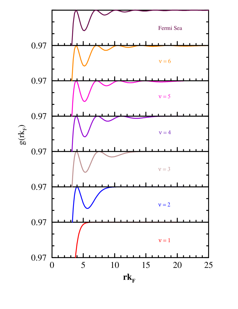
FIG. 1.: Pair distribution function for non-interacting electrons at integer filling factors ($\nu=n$) and also for the Fermi sea.

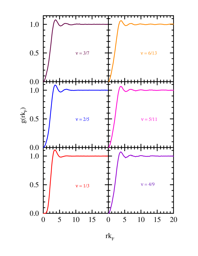
FIG. 2.: Pair distribution functions for several FQHE states at $\nu=n/(2n+1)$, corresponding to $n$ filled Landau levels of composite fermions. $N=$ 50, 54, 60, 60, 60, and 54 particles have been used for $n=$ 1, 2, 3, 4, 5, and 6, respectively. The statistical error in Monte Carlo is of the order of the noise on the curves.

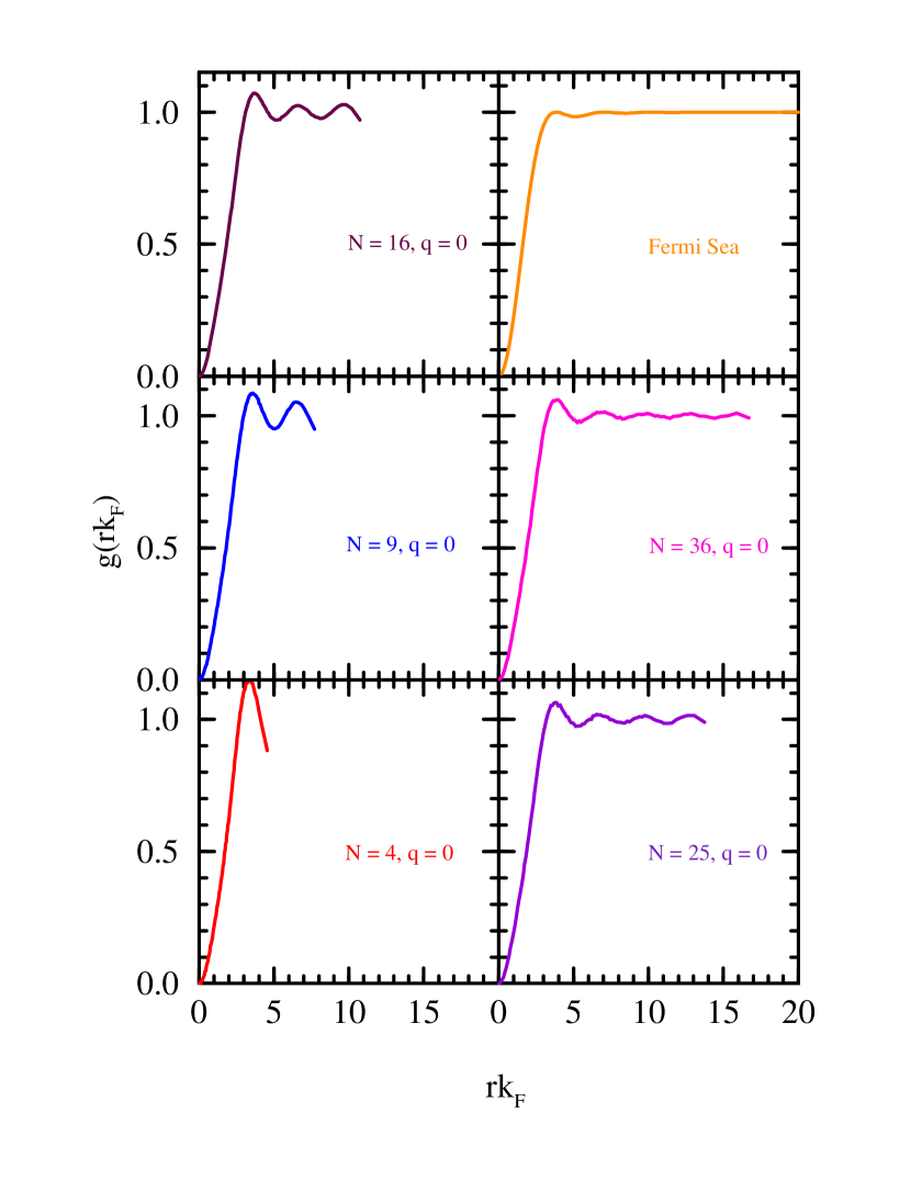
FIG. 3.: Pair distribution functions for several systems of composite fermions at zero effective magnetic field. The number of particles is shown on the figures in each case.

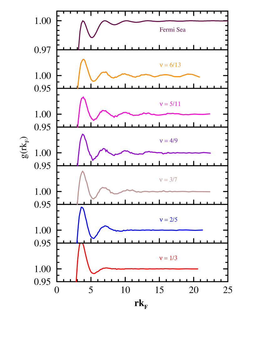
FIG. 4.: A close-up of oscillations in $g(r)$ for filled LLs of composite fermions. The top panel shows the $g(r)$ for non-interacting Fermi sea at zero magnetic field (same as in Fig. 2).

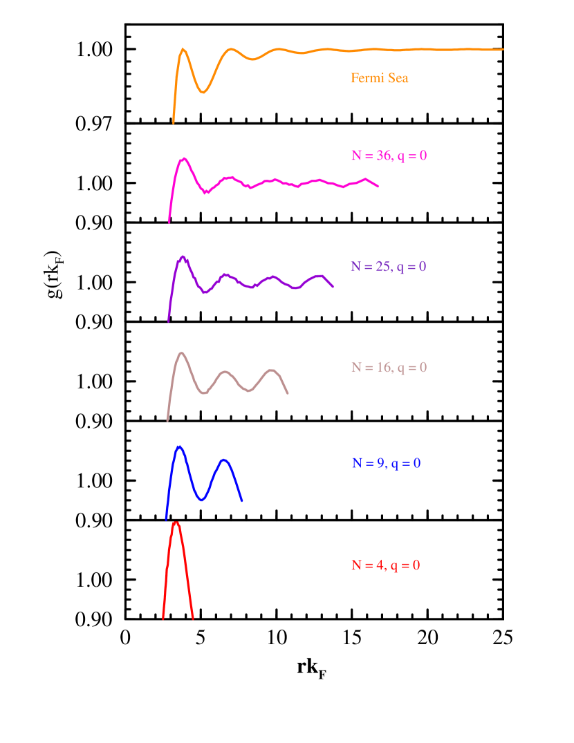
FIG. 5.: Same as Fig. 4 but for composite fermions at vanishing effective magnetic field.

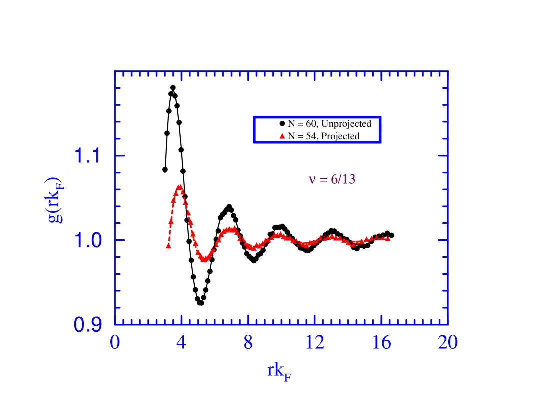
FIG. 6.: The pair correlation function, $g(r)$, for projected as well as the unprojected CF state at $\nu=6/13$. $N=54$ (60) particles were used for the projected (unprojected) CF wave function. The points are the calculated values and the curves are fits according to Eq. (34) with $\alpha=$ 2.75 (2.37), $\beta=$ 2.11 (1.98), $\phi=$ 0.58 (-0.64), and $A=$ 2.71 (3.63) for the projected (unprojected) CF state.

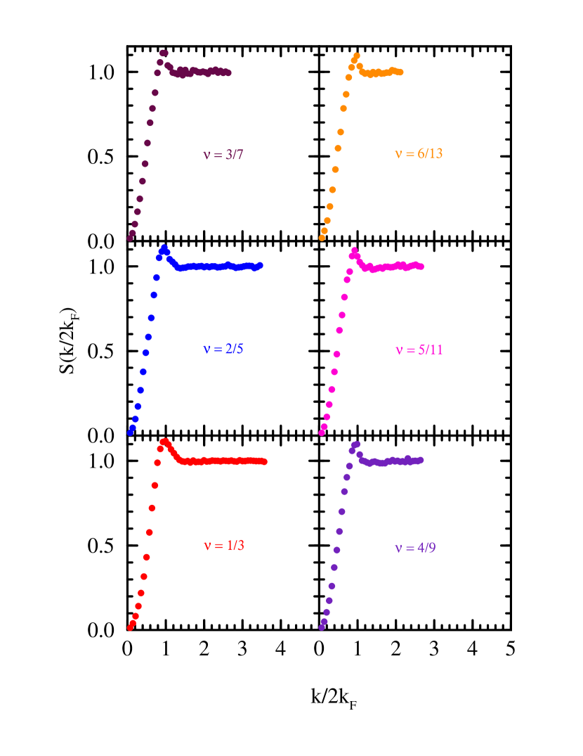
FIG. 7.: Static structure factors for the systems of Fig. 2.

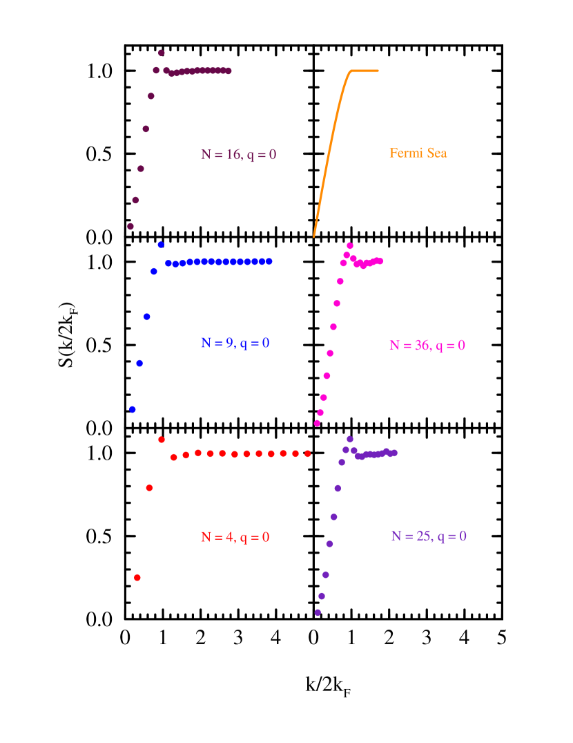
FIG. 8.: Static structure factors for the systems of Fig. 3.

REFERENCES

- [1] See for a review, Perspectives in Quantum Hall Effects, edited by S. Das Sarma and A. Pinczuk (Wiley, New York, 1996).
- [2] J.K. Jain, Phys. Rev. Lett. 63, 199 (1989); Phys. Rev. B 41, 7653 (1990); Science 266, 1199 (1994).
- [3] B.I. Halperin, P.A. Lee, and N. Read, Phys. Rev. B 47, 7312 (1993); B.I. Halperin in [1].
- [4] J.K. Jain and R.K. Kamilla, Phys. Rev. B 55, R4895 (1996).
- [5] G. Dev and J.K. Jain, Phys. Rev. Lett. 69, 2843 (1992); X.G. Wu, G. Dev, and J.K. Jain, ibid. 71, 153 (1993).
- [6] E.H. Rezayi and N. Read, ibid. 72, 900 (1994).
- [7] F.D.M. Haldane, unpublished.
- [8] R.R. Du, H.L. Stormer, D.C. Tsui, L.N. Pfeiffer, and K.W. West, Phys. Rev. Lett. 70, 2944 (1993).
- [9] R.L. Willett et al., Phys. Rev. Lett. 71, 3846 (1993); W. Kang et al., ibid. 71, 3850 (1993); V.J. Goldman et al., ibid. 72, 2065 (1994); J.H. Smet et al., ibid. 77, 2272 (1996).
- [10] A. Lopez and E. Fradkin, Phys. Rev. B 47, 7080 (1993).
- [11] R. Shankar and G. Murthy, unpublished.
- [12] F.D.M. Haldane, Phys. Rev. Lett. 51, 605 (1983).
- [13] F. Stern, Phys. Rev. Lett. 18, 546 (1967); J.K. Jain and P.B. Allen, Phys. Rev. B 32, 997 (1985).
- [14] T.T. Wu and C.N. Yang, Nucl. Phys. B 107, 365 (1976); T.T. Wu and C.N. Yang, Phys. Rev. D 16, 1018 (1977).
- [15] R.B. Laughlin, Phys. Rev. Lett. 50, 1395 (1983).
- [16] For the pair correlation function has been reported earlier in the literature [see, e.g., R. Morf and B.I. Halperin, Phys. Rev. B 33, 2221 (1986)], but recalculated here for completeness.
- [17] See, for example, V. Melik-Alaverdian and N. Bonesteel, Phys. Rev. B 52, R17032 (1996).
- [18] B.L. Altshuler, L.B. Ioffe and A.J. Millis, Phys. Rev. B 50, 14048 (1994).