[

Effect of the Output of the System in Signal Detection

Abstract

We analyze the consequences that the choice of the output of the system has in the efficiency of signal detection. It is shown that the signal and the signal-to-noise ratio (SNR), used to characterize the phenomenon of stochastic resonance, strongly depend on the form of the output. In particular, the SNR may be enhanced for an adequate output.

]

The phenomenon of stochastic resonance (SR) [1, 2, 3, 4, 5, 6, 7, 8, 9, 10, 11] has emerged in the last years as one of the most exciting in the field of nonlinear stochastic systems. Its importance as a mechanism for signal detection has given rise to a great number of applications in different fields, as for example electronic devices [12], lasers[2], neurons [13, 14] and magnetic particles [15, 16].

The most common characterization of SR consists of the appearance of a maximum in the output signal-to-noise ratio (SNR) at non-zero noise level, although different definitions have been used in the literature. The definition through the SNR accounts for practical applications, because the SNR is the quantity that gives the amount of information that can be transfered through a medium as well as measuring the quality of a signal. Additionally, the SNR quantifies the possibility to detect a signal embedded in a noisy environment. Another definition of SR, apparently similar to the one of the SNR, has been proposed in terms of a maximum in the output signal. Although both the SNR and the output signal have been analyzed in terms of the parameters of the system, e.g. the frequency or the amplitude of the input signal, there is an important aspect which has not been considered in depth up to now. An adequate election of the output of the system may have implications in the behavior of the quantities used to manifest the presence of SR. This is precisely the problem we address in this paper.

It is interesting to realize that normally the output of the system is the same as the dynamic variable $x(t)$ entering the stochastic differential equation, although sometimes the sign function of $x(t)$ has also been considered. No matter the system, the output may in general be any function of $x(t)$ which is usually fixed through the characteristics of the problem. However, in order to detect a signal embedded in a noisy environment any function may be used. Thus, instead of Fourier transforming $x(t)$ we can transform the function $v(x(t))$.

Let us discuss one of the most simplest cases, in which the dynamics is described by an Ornstein-Uhlenbeck process, where the input signal modulates the strength of the potential in the following way:

$${dx\over dt}=-h(t)x+\xi(t)\;\;.$$ (1)

Here $h(t)=k(1+\alpha\sin(\omega_{0}t))$, with $k$ and $\alpha$ constants and $\xi(t)$ is Gaussian white noise with zero mean and second moment $\left<\xi(t)\xi(t+\tau)\right>=D\delta(\tau)$, defining the noise level $D$. The effect of this force may be analyzed by the averaged power spectrum

$$P(\omega)={\omega_{0}\over 2\pi}\int_{0}^{2\pi/\omega_{0}}dt\int_{-\infty}^{\infty}\left<v(t)v(t+\tau)\right>e^{-i\omega\tau}d\tau\;\;.$$ (2)

To this end we will assume that it consists of a delta function centered at the frequency $\omega_{0}$ plus a function $Q(\omega)$ which is smooth in the neighborhood of $\omega_{0}$ and is given by

$$P(\omega)=Q(\omega)+S(\omega_{0})\delta(\omega-\omega_{0})\;\;.$$ (3)

Let us now assume the explicit form for the output of the system, $v(x)=|x|^{\beta}$, where $\beta$ is a constant. Although this model does not exhibit SR, it is adequate to illustrate the form in which signal and SNR vary as a function of the output. Considerations about our model based upon dimensional analysis enable us to rewrite the averaged power spectrum as

$$P(\omega,D,k,\alpha,\omega_{0},\beta) = {1\over k}\left({D\over k}\right)^{\beta}q({\omega/\omega_{0}},{k/\omega_{0}},\alpha,\beta)$$ (4)

$$+ \left({D\over k}\right)^{\beta}s({k/\omega_{0}},\alpha,\beta)\delta\left(1-{\omega\over\omega_{0}}\right)\;\;,$$ (5)

where $q({\omega/\omega_{0}},{k/\omega_{0}},\alpha)$ and $s({k/\omega_{0}},\alpha)$ are dimensionless functions.

In spite of the simplicity of this result, a number of interesting consequences can be derived. From Eq. (4) we can obtain the expression for the output signal

$${\rm S}=\left({D\over k}\right)^{\beta}s({k/\omega_{0}},\alpha,\beta)\;\;.$$ (7)

Three qualitative different situations are present depending on the exponent $\beta$. For $\beta>0$ the signal diverges when the noise level $D$ goes to infinity, whereas for $\beta<0$ the signal diverges when $D$ goes to zero. Even more interesting is the case $\beta=0$, in which the signal does not depend on the noise level. The previous results have been verified numerically for some particular values of $\beta$ (Fig. 1), by integrating the corresponding Langevin equation following a standard second-order Runge-Kutta method for stochastic differential equations [17, 18].

FIG. 1.: Output signal corresponding to Eq. (1) ($k=1$, $\alpha=0.5$, and $\omega_{0}/2\pi=0.1$) for different exponents of the output ($\beta=-0.5,0,1,2,5$). The lines are fit to a power law ($\beta_{fit}=-0.501,0.001,0.998,1.996,4.993$).

FIG. 2.: Time evolution of $x(t)^{2}$ (same situation as in Fig. 1) for the noise levels (a) $D=0.01$ and (b) $D=1$.

It is interesting to point out that the signal increases for low or high noise intensities, depending on the value of the exponent $\beta$. From the previous considerations it becomes clear that the output signal itself does not always constitute a useful quantity to elucidate the optimum noise level to detect a signal. In contrast, the SNR overcomes this ambiguity. Its expression straightforwardly follows from Eq. (4)

$${\rm SNR}=k{s({k/\omega_{0}},\alpha,\beta)\over q({\omega/\omega_{0}},{k/\omega_{0}},\alpha,\beta)}\;\;,$$ (8)

This result does not depend on the noise level thus indicating that the system is insensitive to the noise. No matter the noise intensity, the SNR has always the same value despite the fact that signal is a monotonic increasing or decreasing function of the noise. For further illustration of these features we have depicted in Fig. 2. the temporal evolution of the output of the system when $v(x)=x^{2}$, for two values of the noise level. In both cases we have used the same realization of the noise. In the figure, we can see how the noise only affects the system by changing its characteristic scales.

The former results refer to the behavior of the SNR as a function of $D$. For practical applications it is also interesting the knowledge of the SNR as a function of $\beta$ based upon the possible increasing of the SNR when varying $\beta$. We have found that the SNR has a maximum at $\beta=1$ (see Fig. 3). Consequently, for the output class of functions $v(x)=|x|^{\beta}$ the input signal will be better detected when $\beta=1$.

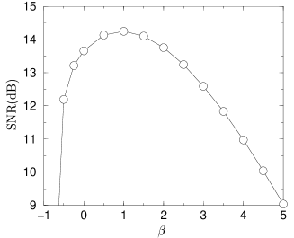
FIG. 3.: SNR as a function of the exponent of the output (same situation as in Fig. 1).

All the functions we are considering as outputs are scale invariant, and dimensional analysis can be readily performed. However, when this requirement about $v(x)$ does not holds, the previous results do not apply. This could be the case of the Heaviside step function $v(x)=\Theta(x-\theta)$, where $\theta$ represents a threshold. In fact, this situation is quite similar to standard threshold devices [9] considered previously. In this case, both the SNR and the output signal exhibit a maximum at non-zero noise level (see Fig. 4). Although the evolution equation of the variable $x(t)$ is linear, SR appears due to the fact that the output is a nonlinear function.

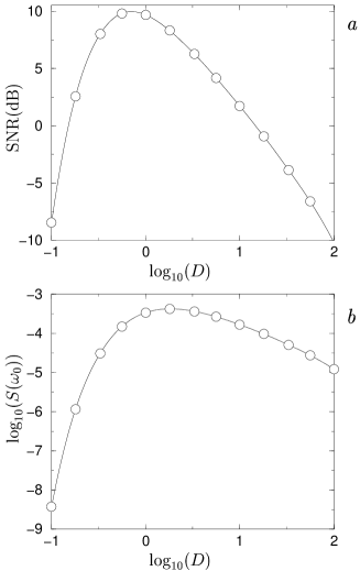
FIG. 4.: (a) SNR and (b) output signal for the output equal to the step function with threshold $\theta=1$ (same situation as in Fig. 1).

Having discussed the role played by the output in a simple monostable system, let us now analyze the case of the bistable quartic potential, which has been frequently proposed in order to describe the phenomenon of SR. The dynamics of the system is then given by the following equation:

$${dx\over dt}=ax-bx^{3}+A\sin(\omega_{0}t)+\xi(t)$$ (9)

where a, b and $A$ are constants and $\xi(t)$ is the same noise as the one introduced through Eq. (1).

To study this system, one usually takes as output the variable $x(t)$ and sometimes the sign function ${\rm sgn}(x(t))$. In the limit when the amplitude of the input signal goes to zero, these two forms of the output give the same results (see ref. [3] for more details). However, when the input signal has a finite amplitude, the SNR for $x(t)$ diverges, whereas for ${\rm sgn}(x(t))$ goes to zero when the noise level decreases. Despite the divergence of the SNR for $x(t)$, if the amplitude of the input signal is not large enough, the SNR has a maximum at non-zero $D$.

As output, we could take in general $x(t)^{\beta}$. The choice of $\beta$ has important consequences as the SNR may depend on this parameter. Thus to better detect a signal, the noise level is not necessarily the only tunable parameter. In Fig. 5(a) we have plotted the SNR for different values of $\beta$, observing its strong dependence on this parameter. In particular, for $\log_{10}(D)\approx-1.25$, upon varying $\beta$ from $1$ to $7$ the SNR increases in about 12 dB. Moreover, when increasing $\beta$ the maximum in the SNR becomes less pronounced and disappears for a sufficiently large $\beta$, as occurs for the case $\beta=25$ . In regards to the signal, variations of $\beta$ change its behavior drastically. This point is illustrated in Fig. 5(b) where we can see that, when increasing the noise level, for $\beta=1$ the signal goes to zero, whereas for the remaining cases the signal always increases at sufficiently high noise level. In Fig. 5(c) we have also displayed the output noise. From Fig. 5(a) it follows that a simple variation on the output changes the qualitative form of the SNR, in such a way that the maximum at non-zero noise level may disappear. Thus, the SNR is a monotonic decreasing function of $D$ and apparently the input signal can always be better detected by decreasing the noise level. However, when the SNR is a decreasing function of $D$, there exists a region around the maximum, corresponding to the curves $\beta=1,3,5,7$ in which the SNR for $\beta=1,3,5,7$ is greater than that for $\beta=25$. We then conclude that when increasing the noise level, the signal can be better detected if one simultaneously changes the value of $\beta$.

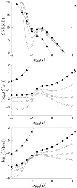
FIG. 5.: (a) SNR, (b) output signal, and (c) output noise for the bistable quartic potential ($a=1$, $b=1$, $\omega_{0}/2\pi=0.1$ and $A=0.13$) for the outputs $\beta=1$ (empty circles), $\beta=3$ (empty triangles), $\beta=5$ (empty squares), $\beta=7$ (filled circles), and $\beta=25$ (filled triangles).

To end our analysis, in Fig. 6 we have displayed two temporal series for two different values of $\beta$ at the noise level for which the effect of the variation on $\beta$ is more pronounced. We can see that intrawell oscillations, for $\beta=7$ are better observed than for $\beta=1$. This fact explains the increase of the SNR.

FIG. 6.: Time evolution of (a) $x(t)$ and (b) $x(t)^{7}$ (same situation as in Fig. 5) for the noise level $D=0.056$. The sinusoidal line in both figures indicates the value of $h(t)$.

In summary, we have shown that the quantities (signal and SNR) used to characterize the phenomenon of SR strongly depend on the form of the output. In this regard, the behavior of the SNR has revealed to be more robust than the one corresponding to the signal. Our findings have important applied aspects since an adequate choice of the output of the system may be crucial in order to better detect a signal.

This work was supported by DGICYT of the Spanish Government under Grant No. PB96-0881. J.M.G.V. wishes to thank Generalitat de Catalunya for financial support.

REFERENCES

- [1] R. Benzi, A. Sutera, and A. Vulpiani, J. Phys. A 14, L453 (1981).
- [2] B. McNamara, K. Wiesenfeld, and R. Roy, Phys. Rev. Lett. 60, 2626 (1988).
- [3] B. McNamara and K. Wiesenfeld, Phys. Rev. A 39, 4854 (1989).
- [4] A. Simon and A. Libchaber, Phys. Rev. Lett. 68, 3375 (1992).
- [5] Proceedings of the NATO Advanced Research Workshop on Stochastic Resonance, San Diego, 1992 [J. Stat. Phys. 70, 1 (1993)].
- [6] F. Moss, in Some Problems in Statistical Physics, edited by G. H. Weiss (SIAM, Philadelphia,1994).
- [7] K. Wiesenfeld, D. Pierson, E. Pantazelou, C. Dames, and F. Moss, Phys. Rev. Lett. 72, 2125 (1994).
- [8] K. Wiesenfeld and F. Moss, Nature 373, 33 (1995).
- [9] Z. Gingl, L. B. Kiss, and F. Moss, Europhys. Lett. 29, 191 (1995).
- [10] F. Marchesoni, L. Gammaitoni, and A. R. Bulsara, Phys. Rev. Lett. 76, 2609 (1996).
- [11] J. M. G. Vilar and J. M. Rubí, Phys. Rev. Lett. 77, 2863 (1996)
- [12] S. Fauve and F. Heslot, Phys. Lett. A 97 5, (1983).
- [13] A. Longtin, A. Bulsara, and F. Moss, Phys. Rev. Lett. 67, 656 (1991).
- [14] J. K. Douglass, L. Wilkens, E. Pantazelou, and F. Moss, Nature 365, 337 (1993).
- [15] A. Peréz-Madrid and J.M. Rubí, Phys. Rev. E 51, 4159 (1995).
- [16] A.N. Grigorenko, P.I. Nikitin, A.N. Slavin, and P.Y. Zhou, J. Appl. Phys. 76, 6335-6337 (1994).
- [17] P. E. Kloeden and R. A. Pearson, J. Austral. Math. Soc., Ser B, 20, 8 (1977).
- [18] J. R. Klauder and W. P. Petersen, SIAM J. Numer. Anal. 22, 1153 (1985).