[

Stochastic Multiresonance

Abstract

We present a class of systems for which the signal-to-noise ratio as a function of the noise level may display a multiplicity of maxima. This phenomenon, referred to as stochastic multiresonance, indicates the possibility that periodic signals may be enhanced at multiple values of the noise level, instead of at a single value which has occurred in systems considered up to now in the framework of stochastic resonance.

]

In recent years, the phenomenon of stochastic resonance (SR) has been subject of intense activity, to the extent that many examples have been found in different scientific areas [1, 2, 3, 4, 5, 6, 7, 8, 9, 10, 11, 12, 13, 14, 15]. The phenomenon has been characterized by the appearance of a maximum in the output signal-to-noise ratio (SNR) at a non-zero noise level. In this sense, noise plays a constructive role since an optimized amount is responsible for the enhancement of the response of the system to a periodic signal, which otherwise would be manifested with more difficulty. In spite of the efforts devoted to its understanding, there is an aspect which has not been considered up to now. Under some circumstances, the SNR may display a multiplicity of maxima and hence, there is a set of values of the noise level at which the response of the system is enhanced. In this Letter we address precisely this possibility for the appearance of those maxima, then we show that the concept of SR is more general than the one we already know. In this regard, we have found a class of systems whose output SNR is a non-trivial periodic function of the logarithm of the noise level. Similarly, our analysis also reveals that the SNR as a function of the noise level may exhibit any number of maxima.

Consider systems with only one relevant degree of freedom whose dynamics is described by the following Langevin equation

$${dx\over dt}=-f(x,t)x+\sqrt{D}\xi(t)\;\;,$$ (1)

where $f(x,t)$ is a given function, $\xi(t)$ is Gaussian white noise with zero mean and second moment $\left<\xi(t)\xi(t^{\prime})\right>=\delta(t-t^{\prime})$, and $D$ is a constant defining the noise level. Here the input signal enters the system through $f(x,t)$, and we will assume it to be periodic in time with frequency $\omega_{0}$. The output of the system is given by $v(x)=|x|^{n}$, with $n$ a positive constant. The SNR is defined, as usual, by

$$\mbox{SNR}=S(\omega_{0})_{v(x)}/N(\omega_{0})_{v(x)}\;\;,$$ (2)

where $S(\omega_{0})_{v(x)}$ and $N(\omega_{0})_{v(x)}$ are the output signal and output noise corresponding to $v(x)$, respectively.

Under the transformation $\tilde{x}=e^{\gamma}x$ and $\tilde{D}=e^{2\gamma}D$, with $\gamma$ constant, Eqs. (1) and (2) remain unchanged if

$$f(x,t)=f(xe^{\gamma},t)\;\;.$$ (3)

Consequently, for the class of systems for which the previous equality holds, for a certain value of $\gamma$, the SNR has the same value at D and at $e^{2\gamma}D$. This fact occurs when $f(x,t)=q(\ln(x),t)$, where $q$ is a periodic function of its first argument, with periodicity $\gamma$ if $\gamma$ is the lower positive number satisfying Eq. (3). Therefore, the SNR is a periodic function of the logarithm of the noise level. Notice that both the signal and noise are not invariant under this transformation, but they are changed in the following fashion

$$S(\omega_{0})_{v(\tilde{x})} = e^{2\gamma n}S(\omega_{0})_{v(x)}\;\;,$$ (4)

$$N(\omega_{0})_{v(\tilde{x})} = e^{2\gamma n}N(\omega_{0})_{v(x)}\;\;.$$ (5)

In order to illustrate the previous results we have analyzed some representative explicit expressions of $f(x,t)$. To this purpose we have numerically integrated the corresponding Langevin equation by means of a standard second-order Runge-Kutta method for stochastic differential equations [16]. Moreover, as the output of the system we have used $v(x)=x^{2}$. We will first consider the case in which

$$f(x,t)=\Theta_{T}(\log_{10}(x^{2}))[\beta+\alpha\cos(\omega_{0}t)]$$ (6)

where $\alpha$ and $\omega_{0}$ are constants, and $\Theta_{T}(s)$ is a square wave of period $T$ defined by

$$\Theta_{T}(s)=\left\{\begin{array}[]{lcl}k_{1}&&\mbox{if}\;\sin(2\pi s/T)>0\;\;,\\ k_{2}&&\mbox{if}\;\sin(2\pi s/T)\leq 0\;\;,\end{array}\right.$$ (7)

with $k_{1}$ and $k_{2}$ constants. In Fig. 1(a) we have plotted the SNR corresponding to the previous form of $f(x,t)$, for particular values of the parameters. This figure clearly manifests the periodicity of the SNR as a function of the noise level and the presence of multiple maxima at $D=D_{0}e^{mT}$, with $m$ being any integer number and $D_{0}$ the noise level corresponding to the maximum with $m=0$. We show both the signal and noise in Fig. 1(b). This figure also corroborates the dependence of the signal and noise on $D$ given in Eq. (5).

From this example one can infer the mechanism responsible for the appearance of this phenomenon. Due to the fact that the SNR has dimensions of the inverse of time [15], its behavior is closely related to the characteristic temporal scales of the system. Thus variations of the relaxation time manifest in the SNR. In this example, when $T$ is sufficiently large, for some values of the noise level the system may be approximated by

$${dx\over dt}=-k_{i}[\beta+\alpha\sin(\omega_{0}t)]x+\sqrt{2D}\xi(t)\;\;,$$ (8)

where $i=1,2$, depending on the noise level. In such a situation the SNR is given by

$$\mbox{SNR}=g(\alpha,\omega_{0}k_{i}^{-1})k_{i}\;\;,$$ (9)

with $g$ a dimensionless function [15]. For a sufficiently low frequency, the SNR is proportional to $k_{i}$ ($\mbox{SNR}\approx g(\alpha,0)k_{i}$), i.e. proportional to the inverse of the relaxation time. Consequently, there are two set of values of $D$ for which the SNR differs in approximately $10\log_{10}(k_{1}/k_{2})$ dB, as one can see in Fig. 1(c). We then conclude that multiple maxima in the SNR appears as a consequence of the form in which the relaxation time of the system changes with the noise level.

Let us now consider another explicit expression for $f(x,t)$ that mainly differs from the previous one in the form in which the input signal enters the equation,

$$f(x,t)=k\sin(2\pi\log_{10}(x^{2})/T)+[\beta+\alpha\cos(\omega_{0}t)]\;\;.$$ (10)

Here the spatial and temporal dependence of $f(x,t)$ appears in an additive fashion instead of in a multiplicative way as in Eq. (6). The results for the SNR are shown in Fig. (2) and also corroborate, in this case, the periodic dependence on the logarithm of the noise level.

The importance of the class of systems discussed previously lies in the fact that the periodicity of the SNR can be shown analytically by simple considerations about the invariance of the system under stretching transformations. Numerical analyses have also revealed that the presence of multiple maxima in the SNR as a function of the noise level is a more general phenomenon than the situation described by the equality (3). Thus, the appearance of multiple maxima is robust upon variations of the form of $f(x,t)$. For instance, if the periodicity in $s$ of the function $q(s,t)$ is lost for high and low values of $s$ then the SNR may be a periodic function of $\ln(D)$ for a bounded range of values of $D$. In this regard, we have performed numerical simulations and we have observed that it is possible to obtain any number of maxima depending on the form of $f(x,t)$, even if the periodicity of $q(s,t)$ does not hold for any interval of $s$. As an illustrative example we will analyze a case in which the input signal enters $f(x,t)$ in a additive fashion as well as in Eq. (10).

We will consider that the form of $f(x,t)$ consists of two contributions; namely, one that comes from a time dependent parabolic potential and the other without temporal dependence. Then,

$$f(x,t)=f_{0}(x)+[\beta+\alpha\cos(\omega t)]\;\;.$$ (11)

Parabolic potentials may arise in many physical situations of interest. For instance, around a minimum most of the potentials may be approximated by a parabolic one. Experiments of a temporal variation of the intensity of the potential are common, this is the case of a single dipole under the influence of an external oscillating field [17]. Another remarkable situation described in the same way corresponds to some systems around a bifurcation whose control parameter varies periodically in time, as for example Rayleigh-Bénard convection when the temperature difference between plates varies slowly in a periodic fashion [18, 19]. The term $f_{0}(x)$ may then represent a perturbation to this ideal situation described by only a time-dependent harmonic force.

To be explicit and for the sake of simplicity, we will consider $f_{0}(x)$ to be a linear piecewise function defined by

$$f_{0}(x)=\left\{\begin{array}[]{lcl}k_{1}&&\mbox{if}\;\;|x|\leq c_{1}\;\;,\\ k_{2}&&\mbox{if}\;\;c_{1}<|x|\leq c_{2}\;\;,\\ k_{3}&&\mbox{if}\;\;c_{2}<|x|\leq c_{3}\;\;,\\ k_{4}&&\mbox{if}\;\;c_{3}<|x|\leq c_{4}\;\;,\\ k_{5}&&\mbox{if}\;\;c_{4}<|x|\;\;.\end{array}\right.$$ (12)

In Fig. 3(a) we have depicted the potential $V_{0}(x)$ corresponding to the force $-f_{0}(x)x$ for particular values of the parameters $k_{i}$ and $c_{i}$. It is worth emphasizing that we have considered other forms of $f_{0}(x)$ but the same qualitative results are obtained provided that $f_{0}(x)$ exhibits the main characteristics of Eq. (12), i.e. the potentials must have a similar location of maxima and minima. In Fig. 3(b) we have represented the SNR corresponding to the previous function $f_{0}(x)$ as a function of the logarithm of the noise level. This figure clearly displays two maxima, one more pronounced than the other. Depending on the values of the parameters the second maximum may disappear [Fig. 3(c)] or it can become more pronounced [Fig. 3(d)].

In summary, we have found, for the first time, a class of systems for which the response to a periodic force is enhanced, not only with the addition of an optimized amount of noise, but also at multiple values of the noise level. Thus, the SNR exhibits a series of maxima distributed periodically, as a function of the logarithm of the noise level. This feature has been found to be even more general since any number of maxima may be present. Among others, an applied aspect to be emphasized concerns the possibility for the design of devices for which the enhancement of an external signal may occur at different values of the noise and not only at one particular value. Our findings, then, contribute to a wider understanding of the phenomenon of SR by extending its scope and perspectives, thereby embracing new situations that have not been considered up to now.

This work was supported by DGICYT of the Spanish Government under Grant No. PB95-0881. J.M.G.V. wishes to thank Generalitat de Catalunya for financial support.

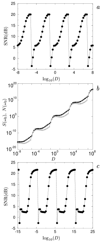
FIG. 1.: (a) SNR corresponding to $f(x,t)$ given through Eq. (6) with parameter values $k_{1}=100$, $k_{2}=1$, $T=4$, $\beta=1$, $\alpha=0.5$ and $\omega_{0}/2\pi=1$. (b) Signal (filled circles) and noise (empty squares) for the previous situation. (c) SNR as in Fig. (a) but with $T=10$.

FIG. 2.: SNR corresponding to $f(x,t)$ given through Eq. (10) parameter values $k_{1}=100$, $k_{2}=1$, with parameter values $k=100$, $T=4$, $\beta=201$, $\alpha=100$ and $\omega_{0}/2\pi=1$.

FIG. 3.: (a) Potential $V_{0}(x)$ corresponding to the force $-f_{0}(x)x$ with parameter values $k_{1}=20$, $k_{2}=-80$, $k_{3}=20$, $k_{4}=-80$, $k_{5}=0$, $c_{1}=1$, $c_{2}=1.73$, $c_{3}=3.16$, and $c_{4}=4.47$. (b) SNR corresponding to $f(x,t)$ given through Eq. (11). The parameter values for $f_{0}(x)$ are the same as in case (a). Moreover $\beta=121$, $\alpha=100$, and $\omega_{0}/2\pi=1$. (c) Same situation as in case (b), except $k_{5}=20$. (d) Same situation as in case (b), except $c_{4}=7.75$.

REFERENCES

- [1] R. Benzi, A. Sutera, and A. Vulpiani, J. Phys. A 14, L453 (1981).
- [2] S. Fauve and F. Heslot, Phys. Lett. A 97, 5 (1983).
- [3] B. McNamara, K. Wiesenfeld, and R. Roy, Phys. Rev. Lett. 60, 2626 (1988).
- [4] B. McNamara and K. Wiesenfeld, Phys. Rev. A 39, 4854 (1989).
- [5] A. Longtin, A. Bulsara, and F. Moss, Phys. Rev. Lett. 67, 656 (1991).
- [6] Proceedings of the NATO Advanced Research Workshop on Stochastic Resonance, San Diego, 1992 [J. Stat. Phys. 70, 1 (1993)].
- [7] J. K. Douglass, L. Wilkens, E. Pantazelou, and F. Moss, Nature 365 337 (1993).
- [8] F. Moss, in Some Problems in Statistical Physics, edited by G. H. Weiss (SIAM, Philadelphia,1994).
- [9] K. Wiesenfeld, D. Pierson, E. Pantazelou, C. Dames, and F. Moss, Phys. Rev. Lett. 72, 2125 (1994).
- [10] K. Wiesenfeld and F. Moss, Nature 373, 33 (1995).
- [11] J. F. Lindner, B. K. Meadows, W. L. Ditto, M. E. Inchiosa, and A. R. Bulsara, Phys. Rev. Lett. 75, 3 (1995).
- [12] Z. Gingl, L. B. Kiss, and F. Moss, Europhys. Lett. 29, 191 (1995).
- [13] M. Grifoni and P. Hanggi, Phys. Rev. Lett. 76, 1611 (1996).
- [14] F. Marchesoni, L. Gammaitoni, and A. R. Bulsara, Phys. Rev. Lett. 76 2609 (1996).
- [15] J. M. G. Vilar and J. M. Rubí, Phys. Rev. Lett. 77, 2863 (1996).
- [16] P. E. Kloeden and E. Platen, Numerical Solution of Stochastic Differential Equations (Springer-Verlag, Berlin, 1995).
- [17] J. M. G. Vilar, A. Peréz-Madrid, and J. M. Rubí, Phys. Rev. E 54, 6929 (1996).
- [18] P. C. Hohenberg and J. B. Swift, Phys. Rev. A 46, 4773 (1992).
- [19] C. W. Meyer, G. Ahlers, and D. S. Cannell, Phys. Rev. A 44, 2514 (1991); 45, 8583 (1992).