Sergei Skorik

Physics Department, Weizmann Institute for Science, Rehovot, Israel

Abstract: We derive an exact expression for the Kubo conductunce in the Quantum Hall device with the point-like intra-edge backscattering. This involves the calculation of current-current correlator exactly, which we perform using form-factor method. In brief, the full set of intermediate states is inserted in the correlator, and for each term the closed mathematical expression is obtained. It is shown that by making a special choice of intermediate states in accordance with the hidden symmetries of the model, one achieves fast convergence of the series, thus proving the form-factor approach to be especially powerfull.
This review is based on the joint work with H.Saleur and F.Lesage.

1 Quantum Hall bar with backscattering and its
quantum field theory representation.

Strongly correlated fermionic systems revealing non-fermi-liquid behavior is one of the most delicate and less studied subjects in mesoscopic physics, mainly because the variety of techniques based on the perturbation theory are not available in the domain of strong interactions. One of the commonly used ways to test such systems is to measure the conductance as a function of voltage and temperature. The behavior of the conductance in the scaling regime of low $V,T$ can to some extent characterize non-fermi-liquid state of the system. On the theoretical level, one can start with some hypothetical effective model, like Luttinger model for 1D electrons, and show that it correctly accounts for the observed physics.

It is believed that a pure Luttinger liquid is realized on the edges of 2D electron gas in the fractional quantum Hall regime. In the number of recent theoretical and experimental works the following problem has been studied. One takes 2D electron gas in the fractional Qunatum Hall regime with $\nu=1/3$ in the two-terminal source-drain geometry shown in Fig. 1 and deforms by static gating potential the narrow region in the middle, so that the boundaries of electron gas come close to each other and start to interact. The quantity of interest is the backscattering current $I_{t}(V,T,\omega,V_{G})$, or the differential conductance $\sigma=dI/dV$. The first experimental data for $I_{t}$ was taken by Milliken, Umbach and Webb. Somewhat more precise experiment was done later by Chang, Pfeiffer and West who used cleaved edge overgrowth technique to measure the tunneling current from the metal to the Quantum Hall edge.

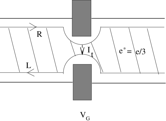
Figure 1: Quantum Hall bar with backscattering between the edge states.

To consider the problem more closely, let us recall first some information about the quantum Hall bar without gating. It is known that when one applies a small voltage difference ($V\ll\omega_{c}$) to the source and drain, the current will be carried by the gapless chiral boundary excitations. Somewhat loose, but nevertheless correct line of arguments for demonstrating this relies on the fact that under Quantum Hall conditons electrons form incompressible droplet. The change of its volume will cost a huge amount of energy, while the excitations of arbitrary small energy can be produced on the boundary of the droplet, by creating some local lump. It was shown by Wen that the low-energy edge excitations can be described by the following effective (1+1)-dimensional Hamiltonian density:

$${\cal{H}}_{0}={1\over 8\pi}[\pi^{2}(x)+(\partial_{x}\phi)^{2}]$$ (1)

where $\pi(x)$ is the momentum conjugated to $\phi$. The field $\phi(x,t)$ represents roughly speaking normal fluctuations of the edge at point $x$ along the edge and can be factorized as $\phi(x,t)=\phi_{L}(t+x)+\phi_{R}(t-x)$, each component describing one of the two edges of the bar. The Hamiltonian (1) represents the energy density of such fluctuations and is similar to the Hamiltonian describing elastic medium. Note that $\phi_{L}$ and $\phi_{R}$ are independent fields, meaning that excitations on two edges are not interacting with each other. The point is that not all eigenstates of the Hamiltonian (1) are real physical excitations observed in the Quantum Hall system. The Hilbert space of eigenstates of (1) is sort of a “playground” which consists of the vacuum $|0\rangle$ and many-particle bosonic states $\phi_{L}(x_{1})...\phi_{R}(x_{N})|0\rangle$ out of which one must select the subspace of physical states. The one-electron excitation is the following state:

$$\Psi^{+}_{L}|0\rangle=:e^{i\phi_{L}/\sqrt{\nu}}:|0\rangle,\qquad\Psi^{+}_{R}|0\rangle=:e^{i\phi_{R}/\sqrt{\nu}}:|0\rangle$$ (2)

and the electric charge along the edge is given by the following operators:

$$Q_{L}=e\int:\Psi_{L}^{+}\Psi_{L}:=e\sqrt{\nu}\int\partial_{x}\phi_{L},\qquad Q_{R}=e\int:\Psi_{R}^{+}\Psi_{R}:=-e\sqrt{\nu}\int\partial_{x}\phi_{R}$$ (3)

It is said that $\Psi^{+}_{L}(\Psi^{+}_{R})$ creates an electron on the left (right) edge, which is represented by the commutation relation $[\Psi_{L},Q_{L}]=e\Psi_{L}$. The correct anticommutator $\{\Psi_{L,R}^{+}(x),\Psi_{L,R}(x^{\prime})\}=\delta(x-x^{\prime})$ is ensured by the normal ordering of exponential and by $[\phi_{L,R}(x),\phi_{L,R}(x^{\prime})]=\pm i\pi sign(x-x^{\prime})$ (such a representation of fermions in terms of free bosonic states is known as bosonization).

Beside electrons, there exist quasiparticle excitations with the fractional charge $e^{\ast}=\nu e$. The quasiparticles are created by the operators similar to those of electrons, with $\nu\to 1/\nu$ in the exponent:

$$\Psi^{+}_{qL}|0\rangle=:e^{i\sqrt{\nu}\phi_{L}}:|0\rangle,\qquad\Psi^{+}_{qR}|0\rangle=:e^{i\sqrt{\nu}\phi_{R}}:|0\rangle$$ (4)

The gating of the bar allows for the scattering of electrons and quasiparticles from one edge to another through intermediate impurities in the region where two edges are close to each other. Under the assumption that the scattering takes place at one point, $x=0$, we write down the most general term decsribing many-particle backscattering processes:

$$H_{bs}=\sum_{n=1}^{\infty}b_{n}[\Psi_{qL}^{+}\Psi_{qR}]^{n}(0)+h.c.=\sum_{n=1}^{\infty}b_{n}\cos[n\sqrt{\nu}(\phi_{L}-\phi_{R})]_{x=0}$$ (5)

In particular, the $n=1$ term is just one quasiparticle tunneling process, and $n=1/\nu$ term is electron tunneling. The form of (5) suggests that quasiparticles are more fundamental objects than electrons, the electron tunneling simply being the coherent tunneling of $1/\nu$ quasiparticles. Further, the renormalization group analysis shows that in the limit of small energy scales (large distances) the correlation functions of the $H_{0}+H_{bs}$ system are exactly the same as the low energy correlation functions of the Hamiltonian

$$H={1\over 8\pi}\int_{-\infty}^{+\infty}dx[\pi^{2}(x)+(\partial_{x}\phi)^{2}]+b_{1}\cos[\sqrt{\nu}(\phi_{L}-\phi_{R})]_{x=0}$$ (6)

This is the basic theoretical model, derived in the pioneering work by Wen. We show in the following sections how to obtain exactly expression for the linear response $\sigma(\omega,b_{1})$ for $T=0$ using Kubo’s formula and the model (6).

2 Mapping to a half-line.

The Hamiltonian (6) is a particular form of 1D field theory with impurity. After making a canonical transformation on the fields one can rewrite (6) as a theory on a half-line with a boundary interaction. The reason for doing this will become clear later. Introduce

$$\phi_{1}(x+t) = {1\over\sqrt{2}}\left[\phi_{L}(x,t)+\phi_{R}(-x,t)\right]$$

$$\phi_{2}(x+t) = {1\over\sqrt{2}}\left[\phi_{L}(x,t)-\phi_{R}(-x,t)\right]$$ (7)

As a result, field $\phi_{1}$ decouples from $\phi_{2}$ as a free field, while $\phi_{2}$ bears all the interactions.
Remark: With the backscattering of the form (5) the total electric charge on two edges, $Q_{L}+Q_{R}$, is still conserved, although $Q_{L}$ and $Q_{R}$ are not conserved separately. It is easy to check that $Q_{L}+Q_{R}$ is expressed purely in terms of field $\phi_{1}$, while $Q_{L}-Q_{R}$ depends only on $\phi_{2}$.

Further, one folds the line by defining a new field, $\Phi=\Phi_{L}+\Phi_{R}$ on a half-line as follows:

$$\Phi_{L}(x,t) = {1\over 2\sqrt{\pi}}\phi_{2}(x+t),\quad x>0,$$

$$\Phi_{R}(x,t) = {1\over 2\sqrt{\pi}}\phi_{2}(-x+t),\quad x>0.$$ (8)

So, we arrive to the boundary sine-Gordon Hamiltonian

$$H={1\over 2}\int^{\infty}_{0}dx[\Pi^{2}(x)+(\partial_{x}\Phi)^{2}]+b\cos{\sqrt{8\pi\nu}\over 2}\Phi(0),$$ (9)

3 Definition of the boundary state.

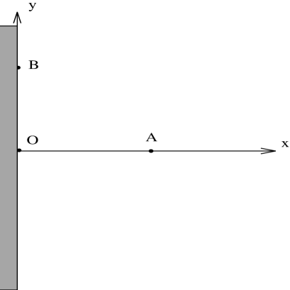
Figure 2: The geometry of space-time.

We will work on the half-plane which geometry is shown in Figure 2. Based on the euclidean duality, there are two alternative ways to introduce the Hamiltonian picture. First, one can take $x$ to be euclidean time. In this case the equal time section is an infinite line $x=$const, $y\in(-\infty,\infty)$. Hence the associated space of states is the same as in the bulk theory. In our case the bulk theory related to the Hamiltonian (9) is just a massless free boson on the line:

$$H={1\over 2}\int^{\infty}_{-\infty}dx[\Pi^{2}(x)+(\partial_{x}\Phi)^{2}],$$ (10)

obtained from (9) by changing the roles of space and time. The boundary term at $x=0$ dissapears from the Hamiltonian, but appears as the “time boundary,” or initial condition at $x=0$ which is described by the boundary state $|B\rangle$ (a particular state from the bulk Hilbert space). The correlators are expressed as

$$\langle O_{1}(x_{1},y_{1})...O_{N}(x_{N},y_{N})\rangle={\langle B|{\cal T}_{x}[O_{1}(x_{1},y_{1})...O_{N}(x_{N},y_{N})]|0\rangle\over\langle 0|B\rangle},$$ (11)

where $O_{i}(x,y)$ are the Heisenberg local field operators

$$O_{i}(x,y)=e^{-xH}O_{i}(0,y)e^{xH},$$ (12)

and ${\cal T}_{x}$ means x-ordering.

Alternatively, one can take the direction along the boundary to be the time. In this case boundary appears as a boundary in space, and the Hilbert space of states is associated with the semi-infinite line $y=$const, $x\in[0,\infty)$. The correlation functions of any local fields $O_{i}(x,y)$ can be computed in this picture as the matrix elements

$$\langle O_{1}(x_{1},y_{1})...O_{N}(x_{N},y_{N})\rangle={\langle 0||{\cal T}_{y}[O_{1}(x_{1},y_{1})...O_{N}(x_{N},y_{N})]||0\rangle\over\langle 0||0\rangle},$$ (13)

where $||0\rangle$ is the ground state of the boundary Hamiltonian, $O_{i}(x,y)$ are understood as the corresponding Heisenberg operators

$$O_{i}(x,y)=e^{-yH_{B}}O_{i}(x,0)e^{yH_{B}},$$ (14)

and ${\cal T}_{y}$ means y-ordering.

The equality of expressions (11) and (13) can be understood as a definition of the boundary state, which is chosen such as to provide the equivalence of correlators. Ghoshal and Zamolodchikov found the generic form of the boundary state for the special class of models, called integrable, including the model of our interest (9):

$$|B\rangle=|0\rangle+\sum_{N=1}^{\infty} \int_{-\infty<\theta_{1}<\dots<\theta_{N}<\infty}R^{a_{1}}_{\bar{b}_{1}}\left({i\pi\over 2}+\theta_{1}\right)\dots R^{a_{N}}_{\bar{b}_{N}}\left({i\pi\over 2}+\theta_{N}\right)$$ (15)

$$A_{L}^{a_{N}}(\theta_{N})\dots A_{L}^{a_{1}}(\theta_{1})A_{R}^{b_{1}}(\theta_{1})\dots A_{R}^{b_{N}}(\theta_{N})|0\rangle$$

This expression must be understood as follows: indexes $a_{i},b_{i}$ label the full set of particles which scatter off the boundary with the boundary reflectiom matrices $R^{a}_{b}(\theta)$, and $\bar{b}$ is an antiparticle corresponding to a particle $b$. The summation over the particle indices $a,b$ is assumed. The rapidity $\theta$ parametrizes the momentum of particles as

$$E_{L}=-P_{L}=\mu e^{\theta},\qquad E_{R}=P_{R}=\mu e^{\theta},$$ (16)

with $\mu$ an arbitrary mass scale, and $A_{L,R}^{a,b}(\theta)$ are the operators that create from the vacuum left and right moving particles $a,b$ at rapidity $\theta$. From the structure of the state (5) one can infer what are some of the distinguished properties of the integrable theories: particles scatter off the boundary one by one (without particle production) with their energy preserved.

4 Outline of the method.

We are interested in the AC conductivity at zero temperature which is given by Kubo’s formula

$${\sigma(\omega)=\int_{0}^{\infty}dx\int_{0}^{\infty}\langle 0|j(0)j(t+ix)|0\rangle e^{-i\omega t}dt}$$ (17)

The net current $j$ here is difference of the currents in left and right edges, $j=\partial_{t}\phi_{L}-\partial_{t}\phi_{R}$. Thus, one has to evaluate the correlator $\langle 0|\partial_{t}\phi_{L}(0)\partial_{t}\phi_{R}(x)|0\rangle$ for the model (6) or, equivalently, the correlator $\langle B|\partial_{t}\Phi(0)\partial_{t}\Phi(x)|0\rangle$ for the model (9). In the form-factor approach that we adopt one inserts the full set of intermediate n-particle states in the correlator $\langle B|j(0)j(x)|0\rangle=\sum_{n}\langle B|j(0)|n\rangle\langle n|j(x)|0\rangle$. Then the problem is to find the form-factors $\langle n|j(x)|0\rangle$ and perform the summation over the complete set of intermediate states. For obvious reasons, it is preferred for the intermediate states to take the eigenstates of the Hamiltonian (9).

Let us comment on this last point. In the massless free field theories there is a freedom to choose a complete basis of particle eigen-states. Often, for the basis one takes plane waves, as in the canonical quantization procedure. However, other representations of particle states can be obtained if one regards the massless theory as a limit of certain interacting massive theory. Then, upon switching off bulk interactions and taking the massless limit, one obtains certain massless particle states, remniscent of massive particles, depending from which massive field theory one approaches the massless limit. Of course, one can constract these states as wave packets of certain energy from the plane waves due to the degeneracy of the Hilbert space, but for this one has to know the matrix elements between plane waves and such states, which is not easy to obtain.

Having this in mind, we shall consider the theory (9) as a massless limit of the massive sine-Gordon model:

$$H_{SG}={1\over 2}\int^{\infty}_{-\infty}dx[{\tilde{\Pi}}^{2}(x)+(\partial_{x}\tilde{\Phi})^{2}+m\cos\sqrt{8\pi\nu}\tilde{\Phi}]+\tilde{b}\cos{\sqrt{8\pi\nu}\over 2}\tilde{\Phi}(0)$$ (18)

It was shown by Ghoshal and Zamolodchikov in the work cited above that the model (18) possesses infinite set of mutually commuting local conserved charges. The eigenstates of (18) are well-known massive particles, called kinks, antikinks and their bound states – breathers, which diagonilize the conserved charges. Correspondingly, in the limit $m\to 0$ the conserved charges of (18) become the conserved charges for the model (9) expressed in terms of the massless field $\Phi$, their eigenstates being massless limit of kinks, antikinks and breathers. The major advantage of working in the basis of massless kinks and antikinks is that their boundary scattering matrices are just 2x2 matrices, obtained by Ghoshal and Zamolodchikov exactly. Thus, the boundary state $|B\rangle$ is significantly simplified and given explicitly by expression (5). The integrable models techniques allows also to find exactly the form-factors for the multiparticle kink states. As it is shown below, the summation over the states presents no difficulties, for the series converge rapidly.

The use of relation between (9) and its massive analogue (18) for determining proper particle states, and the hidden symmetries of (9) is the key feature of our approach. Our results are non-perturbative since we do not assume the smallness of the coupling constants $b$ or $\nu$, the expansion parameter being rather a volume of the multi-particle phase space. The hidden symmetries provide the fast convergence of the multi-particle exansion by suppressing the multi-particle creation processes.

5 Calculation of correlation functions

In what follows we will stay with the first representation of correlators, through the boundary state. This means that in Figure 2 coordinate $x$ is imaginary time and $y$ is space coordinate, $z=x+iy$. Time translation is performed by the operator $T=\exp(xH)$, with $H$ being the bulk Hamiltonian (10).

We need compute the following matrix element:

$$\langle B|\partial_{x}\Phi(x_{1},y_{1})\partial_{x}\Phi(x_{2},y_{2})|0\rangle = \langle B|\partial_{z}\Phi_{R}(z_{1})\partial_{\bar{z}}\Phi_{L}(\bar{z_{2}})|0\rangle$$ (19)

$$+ \langle B|\partial_{\bar{z}}\Phi_{L}(\bar{z_{1}})\partial_{z}\Phi_{R}(z_{2})|0\rangle$$

where $\Phi$ is a massless field $\Phi=\Phi_{L}(\bar{z})+\Phi_{R}(z)$ and $|B\rangle$ denotes the boundary state of the sine-Gordon model (9). Because $|B\rangle$ has chirality zero, products of the fields of the same chirality do not contribute to the right hand side of eq. (19).

Substituting the boundary state (5) into (19) and using the fact that left (right) moving field acts only on left (right) moving particles, we obtain the following expansion in terms of the form-factors:

$$\langle B|\partial_{x}\Phi(x_{1},y_{1})\partial_{x}\Phi(x_{2},y_{2})|0\rangle=\langle 0|\partial_{x}\Phi(x_{1},y_{1})\partial_{x}\Phi(x_{2},y_{2})|0\rangle+$$ (20)

$$+ \sum_{N=1}^{\infty}\sum_{a_{i},b_{i}}\mu^{2}\int_{-\infty<\theta_{1}<...<\theta_{N}<\infty}\left[\prod_{i=1}^{N}{d\theta_{i}\over 2\pi}R^{a_{i}}_{\bar{b}_{i}}({i\pi\over 2}+\theta_{i})\right]\langle 0|\Phi_{L}(0)|A^{a_{1}}(\theta_{1}),...,A^{a_{N}}(\theta_{N})\rangle_{L}$$

$$\times \langle 0|\Phi_{R}(0)|A^{b_{1}}(\theta_{1}),...,A^{b_{N}}(\theta_{N})\rangle_{R}\left(\sum_{i=1}^{N}e^{\theta_{i}}\right)^{2}\left(e^{-(x_{1}+x_{2}+iy_{1}-iy_{2})\mu\left(\sum_{i=1}^{N}e^{\theta}_{i}\right)}+{\rm c.c.}\right)$$

$$\equiv G_{0}(z_{1}-z_{2})-\sum_{n=1}^{\infty}I_{n}$$

The first term in (20), $G_{0}$, is the Green’s function of the free massless scalar (10) on the plane:

$$G_{0}(z,\bar{z})={1\over 4\pi}\left({1\over z^{2}}+{1\over\bar{z}^{2}}\right)$$ (21)

Obviously, it depends only on the difference of the points, while the rest of the terms $I_{n}$ depend on $x_{1}+x_{2}$ as a consequence of the translational invariance breakdown on the half-plane.

The particle spectrum in (20) is determined by the model (18) for $\nu=1/3$ and consists of a massless kink $A^{+}(\theta)$, anti-kink $A^{-}(\theta)=\bar{A}^{+}(\theta)$, and a massless breather $A^{0}(\theta)$. Corresponding boundary reflection matrices are:

$$R^{0}_{0}(\theta) = -\tanh{1\over 2}(\theta-\theta_{B}-{i\pi\over 2})$$

$$R^{\pm}_{\mp}(\theta) = e^{\sqrt{8\pi/3}}D(\theta-\theta_{B}),$$

$$R^{\pm}_{\pm}(\theta) = e^{-\sqrt{8\pi/3}}D(\theta-\theta_{B}),$$ (22)

$$D(\vartheta)={1\over 2\cosh(\vartheta-{i\pi\over 4})}{\Gamma({3\over 8}-{i\vartheta\over 2\pi})\Gamma({5\over 8}+{i\vartheta\over 2\pi})\over\Gamma({5\over 8}-{i\vartheta\over 2\pi})\Gamma({3\over 8}+{i\vartheta\over 2\pi})}$$ (23)

The impurity coupling constant $b$ enters the correlator only through the above scattering matrices, and we parametrized $b(T_{B})$ in terms of the boundary temperature $T_{B}=\mu e^{\theta_{B}}$. The $b=0$ point corresponds to $\theta_{B}=-\infty$, while $b=\infty$ corresponds to $\theta_{B}=\infty$. The momentum and boundary temperature enter the scattering matrices in the dimensionless combination $P/T_{B}$, which means that $R^{a}_{b}$ depend on the difference $\theta-\theta_{B}$. The form-factors $\langle 0|\Phi_{L,R}(0)|A^{a_{1}}(\theta_{1}),...,A^{a_{N}}(\theta_{N})\rangle_{L,R}$ have been obtained by Smirnov.

The first term, $I_{1}$, in (20) is the one-breather contribution. The corresponding form-factors $\langle 0|\Phi_{L}(0)|A^{0}(\theta)\rangle_{L}$ and $\langle 0|\Phi_{R}(0)|A^{0}(\theta)\rangle_{R}$ are just constants. Explicitly, we have

$$I_{1}={\mu^{2}\over 2N_{0}}\int_{-\infty}^{+\infty}{d\theta\over 2\pi}e^{2\theta}\left(e^{-(x_{1}+x_{2}-iy_{1}+iy_{2})\mu e^{\theta}}+{\rm c.c.}\right)\tanh{\theta-\theta_{B}\over 2}$$ (24)

where $N_{0}$ is some normalization constant of the order of 1. Changing variables back to momentum, $p=\mu\exp(\theta)$, it can be rewritten as

$$I_{1}={1\over 4\pi N_{0}}\int_{0}^{\infty}pdp{p-T_{B}\over p+T_{B}}\left(e^{-(z_{2}+\bar{z}_{1})p}+c.c\right)$$ (25)

(the arbitrary mass scale $\mu$ dissapeared from the final answer). Plot of the one-breather contribution to the two-point correlation function for the points OA ($x_{1}=y_{1}=y_{2}=0$) is shown in Figure 3. The three-breather contribution $I_{3}$ related to the form-factors $\langle 0|\Phi_{L,R}(0)|A^{0}(\theta_{1}),...,A^{0}(\theta_{3})\rangle_{L,R}$ is given by

$$I_{3}={\mu^{2}H_{3}^{2}\over 3!N_{0}} \int_{-\infty}^{\infty}\prod_{i=1}^{3}{d\theta_{i}\over 2\pi}\tanh{\theta_{i}-\theta_{B}\over 2}$$

$$\times \prod_{i<j}^{3}{|F_{min}(\theta_{i}-\theta_{j})|^{2}\over 2(1+\cosh(\theta_{i}-\theta_{j}))}\left(\sum_{i=1}^{3}e^{\theta_{i}}\right)^{2}\left(e^{-(z_{2}+\bar{z}_{1})\mu\left(\sum_{i=1}^{3}e^{\theta_{i}}\right)}+c.c\right)$$

where $H_{3}$ is some constant and $F_{min}$ is some complicated known function which we do not specify here. The important fact is that the value of $I_{3}$ is 100 times smaller than $I_{1}$. The term $I_{2}$ is a two-particle contribution of kink and anti-kink, which is related to the form-factors $\langle 0|\Phi_{L,R}(0)|A^{+}(\theta_{1})A^{-}(\theta_{2})\rangle_{L,R}$ (in general, kinks and anti-kinks appear only in pair in the form-factor expansion). The magnitude of this term is approximately 20% of the value of $I_{1}$. Contributing to $I_{3}$ is also the three-particle intermediate state of kink, anti-kink and breather. It is clear how to obtain the rest of the terms. We do not list corresponding expressions here, because $I_{n}$ decrease very fast with $n$ which makes possible to truncate the series for most of the purposes. Each integral $I_{n}$ converges for any finite value of $(x_{1}+x_{2})$, but is divergent for $x_{1}=x_{2}=0$. It is possible to continue analytically our integral representations of $I_{n}$ to the boundary domain $x_{1}=x_{2}=0$ .

Figure 3: Plot of the one-particle contribution to correlator between two points $(0,0)$ and $(x,0)$ as a function of $x$.

6 Scaling from large to small energies.

The non-perturbative nature of the form-factor approach allows one to study the behavior of correlation functions with the change of the scale. Let us study the behavior of integrals $I_{n}$ under the dilatation $z\to e^{\lambda}z$. Such a rescaling can be compensated by the change $\theta_{B}\to\theta_{B}+\lambda$ and by the overall normalization factor $Z(\lambda)=e^{2\lambda}$ to have the integrals (and hence the correlator) unchanged. Repeating this RG transformation, we will flow to the UV or IR fixed points $\theta_{B}=\pm\infty$ (depending whether $\lambda>0$ or $\lambda<0$). For such values of $\theta_{B}$ the hyperbolic tangent factors in the integrands are equal to $\pm 1$, and the integrals are proportional to $\pm 1/z^{2}$. On the plot in Figure 3 one can see two regimes: $\mu z\ll 1$ and $\mu z\gg 1$ when the functions behave as $\pm 1/z^{2}$ (in other words, far away from the boundary an observer will experience the fixed IR boundary condition $\Phi(0)=0$, while very close to the boundary – free UV boundary condition $\partial_{x}\Phi(0)=0$). The non-trivial behaviour at the intermediate scales is due to the presence of boundary, which introduces a scale $\mu e^{\theta_{B}}$ corresponding approximately to the position of the deep. Shifting $\theta_{B}$ corresponds to the motion of the deep to the right or left on Figure 3, untill it will go away completely and one of the regimes will dominate over all scales.

7 Conductivity.

The leading contribution to the conductance computed along the lines of the discussion above for $\nu=1/3$ is given by

$$G(\omega)^{(1)}={1\over 6}-\kappa^{2}{\pi d^{2}\over 8}{\rm Re}\tanh\left[{1\over 2}\log\left({\omega\over\sqrt{2}T_{B}}\right)-{i\pi\over 4}\right]$$ (27)

where $\kappa\approx 3.14$ and $d\approx 0.1414$. We plot the function $G(\omega)^{(1)}$ in Figure 4 and emphasize that it reproduces the shape of the exact condactance to a very high accuracy at any value of coupling $T_{B}(b)$. The higher order terms add some slight corrections to the shape of $G(\omega)^{(1)}$ which are comparable with the available accuracy of experimental measurements (obviously, when probing the conductance in experiment one expects the agreement with the theory for sufficiently small $\omega$; for example when $\omega$ approaches the magnetic gap $\omega_{c}$ the validity of predictions based on the Wen’s theory (6) breaks down).

Figure 4: Frequency dependent conductance at $T=0$.

8 Discussion.

In this methodological review we described a quantum-field theoretical approach to certain impurity problems. The natural question to ask is how generic is this approach, to what extent its applicability is restricted. The above method works for the integrable models, the integrability being a strong constraint. For example, adding another impurity (or another gating potential nearby in the set-up described here) will destroy integrability of the model. However, in such cases one can develop a perturbative expansion over the integrable model by using the ideas given above, in particular by making use of the quasiparticle basis. We hope that such expansions will give better results than perturbations over the free field theory with the plain wave basis. The models that have been so far treated by the above technique or can be treated in principle include Kondo model and its multi-channel analogue, spin-boson model of dissipative quantum mechanics, quantum Hall bar with one or two constrictions, quantum dot and physics of coulomb blockade.