ITP-SB-96-49

We derive rigorous upper and lower bounds for the ground state entropy of the $q$-state Potts antiferromagnet on the honeycomb and triangular lattices. These bounds are quite restrictive, especially for large $q$.

Nonzero ground state disorder and associated entropy, $S_{0}\neq 0$, is an important subject in statistical mechanics; a physical realization is provided by ice, for which $S_{0}=0.82\pm 0.05$ cal/(K-mole), i.e., $S_{0}/k_{B}=0.41\pm 0.03$ [1, 2]. Ground state (g.s.) entropy may or may not be associated with frustration. An early example with frustration is the Ising (equivalently, $q=2$ Potts) antiferromagnet on the triangular lattice [3]. However, g.s. entropy is also exhibited in the simpler context of models without frustration, such as the $q$-state Potts antiferromagnet (AF) [4]-[6] on the square ($sq$) and honeycomb ($hc$) lattices for (integral) $q\geq 3$ and on the triangular ($tri$) lattice for $q\geq 4$. Of these three 2D lattices, $S_{0}$ has been calculated exactly for the triangular case [7], but, aside from the single value $S_{0}(sq,q=3)/k_{B}=(3/2)\ln(4/3)$ [8], not for the square or honeycomb lattices. Therefore, it is valuable to have rigorous upper and lower bounds on this quantity. Using a “coloring matrix” method, Biggs derived such bounds for the square lattice [9]. Here we shall extend his method to derive analogous bounds for the honeycomb lattice and compare the results with our recent Monte Carlo measurements [10, 11] and with large-$q$ series [12]. We also derive such bounds for the triangular lattice; the interest in this case is that the bounds can be compared with the exact result of Baxter [7].

We make use of the fact that the partition function at $T=0$, $Z(\Lambda,q,K=-\infty)$, for the $q$-state zero-field Potts AF on a lattice $\Lambda$ (where $K=\beta J$, $\beta=1/(k_{B}T)$, and $J<0$ denotes the spin-spin coupling) is equal to the chromatic polynomial $P(\Lambda,q)$. Here, $P(G,q)$ is the number of ways of coloring the graph $G$ with $q$ colors such that no adjacent vertices (sites) have the same color [13]. Define the reduced, per site free energy for the Potts AF in the thermodynamic limit as $f(\Lambda,q,K)=\lim_{N\to\infty}N^{-1}\ln Z(\Lambda,q,K)$. From the general relation between the entropy $S$, the internal energy $U$, and the reduced free energy, $S=\beta U+f$ (henceforth, we use units such that $k_{B}=1$), together with the property that $\lim_{K\to-\infty}\beta U(\beta)=0$, as is true of the $q$-state Potts AF models considered here, it follows that $S_{0}(\Lambda,q)=f(\Lambda,q,K=-\infty)=\ln W(\Lambda,q)$, where $W(\Lambda,q)$ is the asymptotic limit

$$W(\Lambda,q)=\lim_{N\to\infty}P(\Lambda,q)^{1/N}$$ (1)

Given this connection, we shall express our bounds on the g.s. entropy $S_{0}(\Lambda,q)$ in terms of the equivalent function $W(\Lambda,q)$. As we have discussed earlier [11], the formal eq. (1) is not, in general, adequate to define $W(\Lambda,q)$ because of a noncommutativity of limits

$$\lim_{N\to\infty}\lim_{q\to q_{s}}P(\Lambda,q)^{1/N}\neq\lim_{q\to q_{s}}\lim_{N\to\infty}P(\Lambda,q)^{1/N}$$ (2)

at certain special points $q_{s}$. We denote the definitions based on the first and second orders of limits in (2) as $W(\Lambda,q)_{D_{nq}}$ and $W(\Lambda,q)_{D_{qn}}$, respectively. This noncommutativity can occur for $q<q_{c}(\Lambda)$, where $q_{c}(\Lambda)$ denotes the maximal (finite) real value of $q$ where $W(\Lambda,q)$ is nonanalytic [11]. Since $q_{c}(hc)=(3+\sqrt{5})/2=2.618...$ and $q_{c}(tri)=4$ (and $q_{c}(sq)=3$) [11], it follows that for the ranges of $q$ considered here, viz., (real) $q\geq 3$ for $\Lambda=hc,sq$ and $q\geq 4$ for $\Lambda=tri$, one does not encounter the noncommutativity (2).

To proceed, we consider a sequence of (regular) $m\times n$   2D lattices of type $\Lambda$, with periodic boundary conditions (PBC’s) in both directions, and $m$ and $n$ even to maintain the bipartite property for finite square and honeycomb lattices and thereby avoid frustration. For $\Lambda=sq$, Biggs introduced the notion of a coloring matrix $T$, somewhat analogous to the transfer matrix for statistical mechanical spin models. The construction of $T$ begins by considering an $n$-vertex circuit $C_{n}$ along a column of $\Lambda$, i.e., a ring around the toroidal lattice, given the PBC’s. The number of allowed $q$-colorings of this circuit is $P(C_{n},q)=(q-1)[(q-1)^{n-1}+(-1)^{n}]$. Now focus on two adjacent columnar circuits, $C_{n}$ and $C_{n}^{\prime}$. Define compatible $q$-colorings of these adjacent circuits as colorings such that no two horizontally adjacent vertices on the circuits have the same color. One can then associate with this pair of adjacent columnar circuits an ${\cal N}\times{\cal N}$ dimensional symmetric matrix $T$, where ${\cal N}=P(C_{n},q)=P(C_{n}^{\prime},q)$ with entries $T_{C_{n},C_{n}^{\prime}}=T_{C_{n}^{\prime},C_{n}}=$ 1 or 0 if the $q$-colorings of $C_{n}$ and $C_{n}^{\prime}$ are or are not compatible, respectively. Then for fixed $m,n$, $P(\Lambda_{m\times n},q)=Tr(T^{m})$. For a given $n$, since $T$ is a nonnegative matrix, one can apply the Perron-Frobenius theorem [14] to conclude that $T$ has a real positive maximal eigenvalue $\lambda_{max,n}(q)$. Hence, for fixed $n$,

$$\lim_{m\to\infty}Tr(T^{m})^{1/(mn)}\to\lambda_{max}^{1/n}$$ (3)

so that

$$W(\Lambda,q)=\lim_{n\to\infty}\lambda_{max}^{1/n}$$ (4)

Denote the column sum $\kappa_{j}(T)=\sum_{i=1}^{\cal N}T_{ij}$ (equal to the row sum $\rho_{j}(T)=\sum_{i=1}^{\cal N}T_{ji}$ since $T^{T}=T$) and $S(T)=\sum_{i,j=1}^{\cal N}T_{ij}$; note that $S(T)/{\cal N}$ is the average row (column) sum. Combining the bounds for a general nonnegative ${\cal N}\times{\cal N}$ matrix $A$, [14]

$$\min\{\gamma_{j}(A)\}\leq\lambda_{max}(A)\leq\max\{\gamma_{j}(A)\}\ ,\quad{\rm for}\quad\gamma_{j}=\kappa_{j}\quad{\rm or}\quad\rho_{j}$$ (5)

with the ($k=1$ case of the ) more restrictive lower bound applicable to a symmetric nonnegative matrix [15],

$$\biggl{[}\frac{S(T^{k})}{\cal N}\biggr{]}^{1/k}\leq\lambda_{max}\ ,\quad{\rm for}\quad k=1,2,...$$ (6)

we have

$$\frac{S(T)}{\cal N}\leq\lambda_{max}(T)\leq\max\{\kappa_{j}(T)\}$$ (7)

For the honeycomb lattice, we find that the analogue of the circuit $C_{n}$ on the square lattice is the set of vertical dimers shown in Fig. 1(a), which we denote as $p$. With $m$ and $n$ even to maintain a bipartite lattice, there are $n/2$ dimers in $p$, and the total number of $q$-colorings of these dimers is $N_{hc,n}=[q(q-1)]^{n/2}$. We next associate the $T$ matrix $T(hc_{n})$ with two adjacent sets of dimers $p$ and $p^{\prime}$ (see Fig. 1(a)); $T(hc_{n})$ is thus a $N_{hc,n}\times N_{hc,n}$ matrix. Two $q$-colorings of the dimer sets $p$ and $p^{\prime}$ are compatible if and only if the horizontally adjacent vertices have different colors, and $T_{p,p^{\prime}}=1$ or 0, respectively, if these colorings are compatible or incompatible. We observe that $S(T)=P(C_{2n},q)$. Therefore,

$$\frac{S(T(hc_{n}))}{N_{hc,n}}=\frac{(q-1)\Bigl{[}(q-1)^{2n-1}+1\Bigr{]}}{[q(q-1)]^{n/2}}$$ (8)

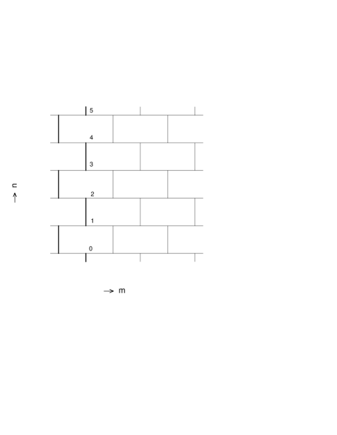
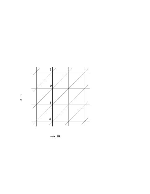
Figure 1: (a) Honeycomb and (b) triangular lattices. See text for discussion.

To calculate the maximal column sum, we consider two neighboring sets of dimers $p$ and $p^{\prime}$, with $n$ sites each labeled by $i=0,1,...,n-1$ (see Fig.1(a)). Let the sites of set $p$ be colored in such a way that sites on the same dimer have different colors (choosing one such configuration of colors corresponds to fixing one column in the color matrix $T$). Let $X_{j}$ denote the number of $q$-colorings of sites $i=0$ to $i=j$ of $p^{\prime}$, such that a site $i$ in set $p$ has a different color from a site $i$ on $p^{\prime}$. If $j$ is odd, the coloring of the $j$’th site in $p^{\prime}$ is only constrained to be different from the coloring of the adjacent $j$’th site in $p$, so $X_{j}=(q-1)X_{j-1}$. [16] The color assigned to an even-$j$ site in $p^{\prime}$ must be different from the color of (i) the other member of the dimer in $p^{\prime}$ and (ii) the adjacent $j$’th site in $p$; hence, $X_{j}=(q-2)X_{j-1}+Y_{j-1}$, where $Y_{j-1}$ denotes the number of colorings for which site $j$ of $p$ has the same color as site $j-1$ of $p^{\prime}$. Note that $Y_{j-1}$ is a subset of $X_{j-2}$, i.e. $Y_{j-1}\leq X_{j-2}$. Thus

$$X_{j}\leq(q-2)X_{j-1}+X_{j-2},\qquad{\rm for\ \ even}\ \ j,\qquad 2\leq j\leq n-2$$ (9)

$$X_{j}=(q-1)X_{j-1}\ ,\qquad{\rm for\ \ odd}\ \ j,\qquad 1\leq j\leq n-1$$ (10)

Using eq.(10) in eq.(9) and setting $j=2\ell$, we have

$$X_{2\ell}\leq\Bigl{[}(q-1)(q-2)+1\Bigr{]}X_{2\ell-2}\ ,\qquad{\rm for}\quad 2\leq 2\ell\leq n-2\ ,$$ (11)

which yields $X_{2\ell}\leq\Bigl{[}(q-1)(q-2)+1\Bigr{]}^{\ell}X_{0}$, where $X_{0}=q-1$. It follows that

$$X_{n-1}=(q-1)X_{n-2}\leq(q-1)^{2}\Bigl{[}(q-1)(q-2)+1\Bigr{]}^{(n-2)/2}$$ (12)

Because $\max\{\kappa_{j}(T(hc_{n})\}\leq X_{n-1}$, we obtain

$$\max\{\kappa(T(hc_{n}))\}\leq(q-1)^{2}[q^{2}-3q+3]^{(n-2)/2}$$ (13)

Hence, using (3) and (4), we derive the bounds

$$\frac{(q-1)^{3/2}}{q^{1/2}}\leq W(hc,q)\leq(q^{2}-3q+3)^{1/2}\quad{\rm for}\quad q\geq 3$$ (14)

The bounds are also seen to apply for the case $q=2$ if one uses as a definition $W(hc,2)\equiv W(hc,2)_{D_{nq}}=1$ given by the first order of limits in eq. (2).

Similarly, for the triangular lattice we define the color matrix $T(tri_{n})$ by considering the compatibility of $q$-colorings of two neighboring $n$-vertex circuits $C_{n}$ and $C_{n}^{\prime}$. An example of such adjacent circuits is shown by the darker lines in Fig. 1(b). Here $T(tri_{n})$ is a $N_{tri,n}\times N_{tri,n}$ matrix, where $N_{tri,n}=P(C_{n},q)=P(C_{n}^{\prime},q)$. For the triangular lattice with periodic or open boundary conditions in the vertical direction, $S(T)$ is equal, respectively, to the numbers $P(cctri_{n},q)$ and $P(octri_{n},q)$ of $q$-colorings of a cyclic or open chain of triangles with $2n$ vertices. In the $n\to\infty$ limit of interest here, $\lim_{n\to\infty}P(cctri_{n},q)^{1/n}=\lim_{n\to\infty}P(octri_{n},q)^{1/n}$, so it does not matter which type of chain we use. An elementary calculation yields

$$P(octri_{n},q)=q(q-1)(q-2)^{2n-2}$$ (15)

so

$$\lim_{n\to\infty}\biggl{[}\frac{S(T(tri_{n}))}{N_{tri,n}}\biggr{]}^{1/n}=\frac{(q-2)^{2}}{q-1}$$ (16)

To calculate $\max\{\kappa_{j}(T(tri_{n}))\}$, we derive, as before, an upper bound for $X_{n-1}$. Each vertex of $C^{\prime}_{n}$ is connected to two vertices of $C_{n}$, hence each of the $X_{j-1}$ colorings of the sites $i=0$ to $i=j-1$ of the circuit $C^{\prime}_{n}$ can be extended in at least $q-3$ ways to the site $i=j$. Thus, for the triangular lattice, the equivalent of eqs. (9) and (10) is

$$X_{j}\leq(q-3)X_{j-1}+X_{j-2},\qquad 2\leq j\leq n-1,$$ (17)

with $X_{0}=q-2$ and $X_{1}\leq(q-3)(q-2)+1$  [17]. This recursion relation is of the same form as the one obtained previously [9] for the square lattice, and can thus be solved by the same method. We thus find for the triangular lattice the inequality

$$\frac{(q-2)^{2}}{q-1}\leq W(tri,q)\leq\frac{1}{2}\Bigl{[}q-3+(q^{2}-6q+13)^{1/2}\Bigr{]}\qquad{\rm for}\qquad q\geq q_{c}(tri)=4$$ (18)

(For $q=3$, the ground state entropy is zero, i.e., $W(tri,3)_{D_{nq}}=1$.)

Denote the lower and upper bounds for these lattices as $W(\Lambda,q)_{\ell}$ and $W(\Lambda,q)_{u}$, respectively. We observe that as $q$ increases, these bounds rapidly approach each other, and hence restrict the exact values $W(\Lambda,q)$ very accurately. This can be seen as a consequence of the fact that, aside from the obvious prefactor $q$, $W(\Lambda,q)_{\ell}$ and $W(\Lambda,q)_{u}$ are the same up to $O(q^{-2})$:

$$q^{-1}W(hc,q)_{\ell}=1-\frac{3}{2}q^{-1}+\frac{3}{8}q^{-2}+\frac{1}{16}q^{-3}+O(q^{-4})$$ (19)

$$q^{-1}W(hc,q)_{u}=1-\frac{3}{2}q^{-1}+\frac{3}{8}q^{-2}+\frac{9}{16}q^{-3}+O(q^{-4})$$ (20)

and similarly with $q^{-1}W(tri,q)_{b}$, $b=\ell,u$. (This was also true for the $\Lambda=sq$ bounds [9]).

In Table 1, we compare the bounds (14) for $\Lambda=hc$ with our recent Monte Carlo measurements of $W(hc,q)$ [10, 11]. We also compare our bounds (18) for $\Lambda=tri$ with the exactly known results of Baxter [7]. For reference, Table 1 includes a similar comparison of the $\Lambda=sq$ bound with the known $q=3$ value [8] and Monte Carlo measurements [18, 19, 11] for $q>3$. We see that as $q$ increases past $q\simeq 4$, the upper and lower bounds bracket the actual respective values quite closely, and that the latter values lie closer to the lower bounds.

$q$	$\frac{W(hc,q)_{\ell}}{W(hc,q)_{MC}}$	$\frac{W(hc,q)_{u}}{W(hc,q)_{MC}}$	$\frac{W(sq,q)_{\ell}}{W(sq,q)}$	$\frac{W(sq,q)_{u}}{W(sq,q)}$	$\frac{W(tri,q)_{\ell}}{W(tri,q)}$	$\frac{W(tri,q)_{u}}{W(tri,q)}$
3	0.98390(60)	1.04358(65)	0.97425(55)	1.05091(60)	$-$	$-$
4	0.99781(60)	1.01612(60)	0.99844(65)	1.03305(65)	0.91262	1.107485
5	0.99948(55)	1.00726(55)	0.99970(60)	1.01593(60)	0.99377	1.06630
6	0.99978(65)	1.00377(65)	0.99992(60)	1.00851(60)	0.99879	1.03087
7	0.99988(65)	1.00220(65)	0.99996(60)	1.00498(60)	0.99963	1.01628
8	0.99999(60)	1.00145(60)	0.99996(65)	1.00312(65)	0.99986	1.00953
9	1.00001(60)	1.00099(60)	0.99995(65)	1.00206(65)	0.99994	1.00602
10	0.99994(60)	1.00063(60)	0.99986(60)	1.00134(60)	0.99997	1.00404

Table 1: Comparisons of lower and upper bounds with Monte Carlo measurements of $W(hc,q)$ and exact values of $W(tri,q)$, respectively, for $q_{c}(\Lambda)\leq q\leq 10$. An analogous comparison is included for $\Lambda=sq$.

To understand why the actual values of $W(\Lambda,q)$ lie closer to the respective lower bounds, we compare the large-$q$ series with the expansions of these lower bounds. For a lattice $\Lambda$ with coordination number $\zeta$, the large $q$ series can be written in the form

$$W(\Lambda,q)=q(1-q^{-1})^{\zeta/2}\;\overline{W}(\Lambda,y)$$ (21)

where $\overline{W}(\Lambda,y)=1+\sum_{n=1}^{\infty}w_{n}y^{n}$ with $y=\frac{1}{q-1}$. Defining the analogous functions $\overline{W}(\Lambda,y)_{b}$ via

$$W(\Lambda,q)_{b}=q(1-q^{-1})^{\zeta/2}\;\overline{W}(\Lambda,y)_{b}\ ,\quad b=\ell,\ u\ ,$$ (22)

we obtain $\overline{W}(hc,y)_{\ell}=1$, which agrees to the first five terms, i.e., to order $O(y^{4})$, with the series [12] $\overline{W}(hc,y)=1+y^{5}+2y^{11}+O(y^{12})$, while $\overline{W}(hc,y)_{u}=1+y^{3}/2+O(y^{6})$. We also calculate $\overline{W}(tri,y)_{\ell}=(1-y^{2})^{2}$, which agrees to the first five terms, i.e. to $O(y^{4})$, with the series expansion of the exact Baxter result, $\overline{W}(tri,y)=1-2y^{2}+y^{4}+y^{5}+O(y^{6})$, while $\overline{W}(tri,q)_{u}=1-2y^{2}+2y^{3}+O(y^{4})$. Finally, $\overline{W}(sq,y)_{\ell}=1+y^{3}$, which agrees to the first seven terms, i.e, to $O(y^{6})$, with the series [12, 19] $\overline{W}(sq,y)=1+y^{3}+y^{7}+O(y^{8})$, while $\overline{W}(sq,y)_{u}=1+2y^{3}+O(y^{4})$.

In summary, we have derived rigorous upper and lower bounds for the (exponent of the) ground state entropy of the Potts antiferromagnet on the honeycomb and triangular lattices and have shown that these are very restrictive for large $q$. Since nonzero ground state entropy sheds light on some of the most fundamental properties of statistical mechanics, it is of interest to derive similar bounds for other lattices; work on this is in progress.

This research was supported in part by the NSF grant PHY-93-09888.

References

• [1] W. F. Giauque and J. W. Stout, J. Am. Chem. Soc. 58, 1144 (1936); L. Pauling, The Nature of the Chemical Bond (Cornell Univ. Press, Ithaca, 1960), p. 466.
• [2] E. H. Lieb and F. Y. Wu, in C. Domb and M. S. Green, eds., Phase Transitions and Critical Phenomena (Academic Press, New York, 1972) v. 1, p. 331.
• [3] G. H. Wannier, Phys. Rev. 79, 357 (1950).
• [4] R. B. Potts, Proc. Camb. Phil. Soc. 48, 106 (1952).
• [5] F. Y. Wu, Rev. Mod. Phys. 54, 235 (1982).
• [6] R. J. Baxter, Exactly Solved Models in Statistical Mechanics (Academic Press, New York, 1982).
• [7] R. J. Baxter, J. Phys. A 19, 2821 (1986); see also R. J. Baxter, ibid. J. Phys. A 20, 5241 (1987).
• [8] E. H. Lieb, Phys. Rev. 162, 162 (1967).
• [9] N. L. Biggs, Bull. London Math. Soc. 9, 54 (1977). The bounds are (q2βˆ’3​q+3)/(qβˆ’1)≀W​(s​q,q)≀(1/2)​[qβˆ’2+(q2βˆ’4​q+8)1/2]superscriptπ‘ž23π‘ž3π‘ž1π‘Šπ‘ π‘žπ‘ž12delimited-[]π‘ž2superscriptsuperscriptπ‘ž24π‘ž812(q^{2}-3q+3)/(q-1)\leq W(sq,q)\leq(1/2)\Bigl{[}q-2+(q^{2}-4q+8)^{1/2}\Bigr{]} for $q\geq 3$.
• [10] R. Shrock and S.-H. Tsai, J. Phys. A 30, 495 (1997).
• [11] R. Shrock and S.-H. Tsai, ITP preprint ITP-SB-96-42 (cond-mat/9612249).
• [12] D. Kim and I. G. Enting, J. Combin. Theory, B 26, 327 (1979). The large-$q$ series expansions of $\overline{W}(\Lambda,y)$ in (21) contain terms with both positive and negative coefficients for each of the lattices considered here.
• [13] R. C. Read and W. T. Tutte, β€œChromatic Polynomials”, in Selected Topics in Graph Theory, 3, eds. L. W. Beineke and R. J. Wilson (Academic Press, New York, 1988).
• [14] See, e.g., P. Lancaster and M. Tismenetsky, The Theory of Matrices, with Applications (New York, Academic Press, 1985); H. Minc, Nonnegative Matrices (New York, Wiley, 1988).
• [15] D. London, Duke Math. J. 33, 511 (1966).
• [16] The restriction on the coloring of site 0 in $p^{\prime}$ will be taken into account automatically by our use of periodic boundary conditions here. Alternatively, one could use an open chain; these choices are equivalent in the $n\to\infty$ limit.
• [17] For cases where the colors on the site $j=1$ and the site below $j=0$ on $C_{n}$ are different, the expression for $X_{1}$ is realized as an equality; if these colors are the same, then it is realized as an inequality.
• [18] X. Chen and C. Y. Pan, Int. J. Mod. Phys. B1, 111 (1987); C. Y. Pan and X. Chen, ibid. B2, 1503 (1988).
• [19] A. V. Bakaev and V. I. Kabanovich, J. Phys. A 27, 6731 (1994).