[

Tunneling and orthogonality catastrophe in the topological mechanism of superconductivity

Abstract

We compute the angular dependence of the order parameter and tunneling amplitude in a model exhibiting topological superconductivity and sketch its derivation as a model of a doped Mott insulator. We show that ground states differing by an odd number of particles are orthogonal and the order parameter is in the d-representation, although the gap in the electronic spectrum has no nodes. We also develop an operator algebra, that allows one to compute off-diagonal correlation functions.

]

1. In the BCS theory of superconductivity numerous physical quantities like London’s penetration depth, the gap in the electronic spectrum, the tunneling amplitude, etc. are expressed through a single object - an off-diagonal two-particle matrix element between ground states with $N$ and $N+2$ particles

$$\Delta(r-r^{\prime})=\varepsilon^{\sigma\sigma^{\prime}}\langle N|c_{\sigma}(r)c_{\sigma^{\prime}}(r^{\prime})|N+2\rangle$$ (1)

This fact is not special to superconductivity, but rather a manifestation of the mean-field character of BCS. In electronic liquids where the interaction is strong in the high temperature regime above $T_{c}$, one expects also to see a difference between these different implementations of superconductivity.

Below we consider the extreme case of a strongly interacting system where a ground state (and the entire spectrum) depends crucially on the number of electrons in the system. In recent years it has been argued that under rather general assumptions, an electronic system where a topological soliton is adiabatically attached to a particle develops superconductivity. Realizations of this phenomenon in low dimensions are Fröhlich ideal conductivity in 1D [1] and anyon superconductivity in 2D [2]. We refer to this phenomenon as topological superconductivity [3, 4]. The crucial features of the mechanism are (i) an electron acquires a geometrical phase in field of a soliton, and a related phenomenon: (ii) orthogonality catastrophe. Both of them make the physics of the superconducting state drastically different from BCS physics and in particular give rise to an angle dependence of the matrix element (1) and the tunneling amplitude.

In this Letter we consider an ideal 2D model of a doped Mott insulator on a square lattice at doping close to the half filling. In this model the Fermi surface consists of four pockets around $k_{f}=(\pm\pi/2,\pm\pi/2)$. We calculate the Josephson tunneling amplitude [5] and show that the phase difference between the tunneling amplitude on the different faces (1,0) and (0,1) of the crystal is $\pi$. At the same time the gap has no nodes. This result is depicted in Fig.1 and is expressed by eq. (14). Although it is in agreement with the corner-SQUID-junction experiment [6] the order parameter is different from the conventional d-wave form. In a forthcoming paper [7] we will show that at incommensurate doping the phase difference between order parameters in the points (1,2) and (3,4) is the twice the angle $\theta$ between vectors ${\bf r}_{1,2}$ and ${\bf r}_{3,4}$.

2. Let us start with a general comment about Josephson tunneling in the presence of orthogonality catastrophe. Let one side of the junction be a BCS superconductor with a small gap and phase $\phi_{0}$. Then the standard Ambegaokar-Baratoff formula gives for the Josephson current $I\sim{\rm Im}\,e^{-i\phi_{0}}\sum_{p_{n}}\int_{0}^{\infty}F(p_{n},\omega)d\omega/\omega$ in terms of the $F$-function of a topological superconductor at momentum $p_{n}$ normal to the surface, $F(p,\omega)=2\pi i\sum\langle N|c_{p\uparrow}|N+1;p\rangle\langle N+1;p|c_{-p\downarrow}|N+2\rangle\delta(\omega-\epsilon_{p})$. In BCS theory the main contribution to the integral comes from intermediate states with an energy of the order of a gap, i.e. a pair is destroyed while tunneling. In a topological superconductor the ground states $|N\rangle$ and low energy states $|N+1\rangle$ have different topological charges and are orthogonal to each other. Their overlap vanishes in the macroscopical system. The $F$-function remains nonzero due to a small contribution of infinitely many states with energy much larger than the gap. As a result, $F$ decays slower than $\omega^{-1}$ (in fact $F(p,\omega)\sim\omega^{-1/2}$), so that $\int dpF(p,\omega)$ is not very small at large $\omega$. Thus, we conclude that the tunneling amplitude is given by the the equal time two-particle matrix element (1) - in contrast to BCS, electron-pairs remain intact while tunneling (for a similar phenomenon see [8]).

3. A number of successive steps [9, 4, 10] have been made over last years towards the derivation of the topological mechanism from an electronic model with an infinite on-site repulsion

$$H=\sum_{\langle ij\rangle}t_{ij}{c}_{i\sigma}^{\dagger}{c}_{j\sigma}+{J}_{ij}{\bf S}_{i}\cdot{\bf S}_{j}\,;\;\;\;{c}_{i\sigma}^{+}{c}_{i\sigma}^{\phantom{+}}\neq 2.$$ (2)

Below we sketch such a derivation and add some new features to take into account spin correlations. The $t-J$ model does not have distinct scales to isolate the physics of topological fluids. To capture the physics of interest we employ an adiabatic approximation, i.e. we treat a hole’s motion in a slowly varying spin background [11].

A single hop of a hole destroys the short range antiferromagnet order. However, two consecutive hops and a spin flip bring the antiferromagnet in order. As a result, the spin configuration remains approximately unchanged, only in second (even) order in the hopping process. In order to treat spins adiabatically we must first integrate out these virtual processes, so that holes remain on the same sublattice (a Schrieffer-Wolf like transformation) [10, 4].

In second order of perturbation theory in $t$ the hopping Hamiltonian is

$${\cal H}=\sum\{c_{\sigma}^{\dagger}(a)t_{\sigma\sigma^{\prime}}(a,a^{\prime})c_{\sigma^{\prime}}(a^{\prime})\\ +c_{\sigma}^{\dagger}(b)t_{\sigma\sigma^{\prime}}(b,b^{\prime})c_{\sigma^{\prime}}(b^{\prime})\}$$

where the sum runs over neighbors $(a,a^{\prime})$ of sublattice A and $(b,b^{\prime})$ of B on a square lattice. The variable hopping amplitudes, say $t_{\sigma\sigma^{\prime}}(a,a^{\prime})$ depend on the spin configuration and are superpositions of chiralities over paths connecting points $a,a^{\prime}$:

$$t_{\sigma\sigma^{\prime}}(a,a^{\prime}) = {\bar{t}}\sum_{b}W_{\sigma\sigma^{\prime}}(a,b,a^{\prime}),$$ (3)

$$W_{\sigma\sigma^{\prime}}(a,b,a^{\prime}) = (\frac{1}{2}+\mbox{\boldmath$\sigma$}\cdot{\bf S}_{a})(\frac{1}{2}+\mbox{\boldmath$\sigma$}\cdot{\bf S}_{b})(\frac{1}{2}+\mbox{\boldmath$\sigma$}\cdot{\bf S}_{a^{\prime}})$$ (4)

where the overall scale for hopping is ${\bar{t}}\sim t^{2}/J$. Now the hopping Hamiltonian is ready for the adiabatic approximation.

First we must find a static spin configuration, i.e. the amplitudes $t(a,a^{\prime})$ to minimize the energy. Their modulus is determined by the competition between electronic and magnetic energies and gives the overall scale of the model. As far as the phase of the hopping amplitudes is concerned we assume that it is determined by the electronic energy alone [11]. The flux hypothesis [9] suggests that, in the leading order in doping, the energy achieves its minimum if the chiralities along contours $a\rightarrow a+e_{i}\rightarrow a+2e_{i}$ are equal in all directions, while chiralities along two different paths connecting sites on the diagonal of a crystal cell have a different sign (the principal of maximal interference) and cancel the amplitude for diagonal hopping:
$\langle W({\bf r},{\bf r}+{\bf e}_{x},{\bf r}+{\bf e}_{x}+{\bf e}_{y})+W({\bf r},{\bf r}+{\bf e}_{y},{\bf r}+{\bf e}_{x}+{\bf e}_{y})\rangle=0,$
$\langle t({\bf r},{\bf r}+{\bf e}_{x}+{\bf e}_{y})\rangle=0,\;\;\;\;\langle t({\bf r},{\bf r}+2{\bf e}_{i})\rangle={1/m}$.

The Fermi-surface of the mean field state consists of four pockets around Dirac points ${\bf k}_{f}\equiv k_{\pm,\pm}=(\pm\frac{\pi}{2},\pm\frac{\pi}{2})$, so we decompose electron operator onto four smooth movers $c_{\sigma}({\bf r})=\sum_{k_{f}}c_{\sigma,\pm\pm}({\bf r})e^{i{\bf k}_{f}{\bf r}}$. In what follows we refer to the smooth functions $c_{\sigma,\pm\pm}({\bf r})$ as to the continuum part and to the factors $e^{i{\bf k}_{f}{\bf r}}$ as to the lattice part of the fermion operator $c_{\sigma}({\bf r})$.

In this basis, the mean field Hamiltonian can be written in a continuum limit as the square of Dirac operator $H=D^{2}=(\alpha_{x}i\partial_{x}+\alpha_{y}i\partial_{y})^{2}$ where the $4\times 4$ Dirac matrices $\{\alpha_{x},\alpha_{y}\}=0$ act in the space labeled by $(\pm\pm)$. The choice of these matrices (gauge freedom) corresponds to a relabeling of the Dirac points and is limited by the symmetry group of the Fermi surface (there are only four different gauges). We choose them to be $\alpha_{x}=\tau_{3}\otimes\tau_{3},\alpha_{y}=\tau_{1}\otimes\tau_{3}$, where the first Pauli matrix $\tau$ acts on the first (x) $\pm$ label and the second acts on the y $\pm$ label. They correspond to the Landau gauge on the lattice with hopping amplitudes $\alpha_{x}\equiv\alpha({\bf r},{\bf r}+{\bf e}_{x})=1,\alpha_{y}\equiv\alpha({\bf r},{\bf r}+{\bf e}_{y})=(-1)^{x}$.

Now we are ready to take into account smooth fluctuations of the phase of the hopping amplitudes (fluctuations of moduli are not that important). The most effective way to do this is to introduce a non-gauge-invariant operator $\psi_{\sigma}$ to describe charge motion and $U(2)$ gauge field ${\bf A}+{\bf\cal A}\cdot\mbox{\boldmath$\sigma$}$ to describe fluctuations of spin chirality $W_{\sigma,\sigma^{\prime}}\sim\exp{i(F+{\bf\cal F}\cdot\mbox{\boldmath$\sigma$}_{\sigma,\sigma^{\prime}})}$, where $F$ and ${\bf{\cal F}}$ are fluxes of $U(1)$ and $SU(2)$ gauge fields. We find the hopping Hamiltonian to be Pauli operator:

$${\cal H}=\frac{1}{2m}\psi^{\dagger}\{(i{\bf\nabla}-{\bf A}-{\bf\cal A}\cdot\mbox{\boldmath$\sigma$})^{2}+\Gamma(F+{\bf\cal F}\cdot\mbox{\boldmath$\sigma$})\}\psi$$ (5)

The second term with $\Gamma=-i\alpha_{x}\times\alpha_{y}$ describes the diagonal hopping due to the fluctuations of chirality.

5. The perturbative vacuum (where the gauge field ${\bf A}$ is small), is unstable when we start to dope the system. The energy achieves its minimum if the Abelian part $F$ of the flux (the topological charge of magnetic solitons) is equal to the number of dopants. The reason for this is that the non negative hopping Hamiltonian (5) in the presence of a static flux acquires states with zero energy [12]. The number of zero modes is twice the number of flux quanta and the density of particles occupying zero modes is adiabatically coupled to the flux: $\rho(r)=2\frac{F}{2\pi}$. The wave functions (non gauge invariant) of zero modes are $\Phi(r)=e^{i\phi-\Gamma\chi}g$ where $A_{z}=\partial_{z}(-i\phi+\chi)$ and $g$ (the lattice part of the zero mode) obeys $\Gamma g=-g$. If the flux is directed up there are two solutions

$$g_{A(B)} = e^{i{\bf k}_{++}\cdot{\bf r}}\pm e^{i{\bf k}_{--}\cdot{\bf r}}+i(e^{i{\bf k}_{-+}\cdot{\bf r}}\pm e^{i{\bf k}_{+-}\cdot{\bf r}})$$ (6)

which are chosen, such that $g_{A}=0$ on sublattice B and $g_{B}=0$ on sublattice A.

While doping, electrons want to create and occupy zero mode states to minimize their energy. This effect competes with the magnetic energy of the flux. Below we assume that the gain in electronic energy wins this competition [7]. As a result two electrons with opposite spins may occupy the same zero mode state. Once zero mode states are occupied, the interaction between them lifts the degeneracy, so that the zero mode states form a narrow band. In a singlet state the band is always completely filled and is detached from the rest of the spectrum, so that the chemical potential lies in a gap $\Delta_{0}$. This results in superconductivity — a density modulation can propagate together with a flux configuration without dissipation, while the electronic spectrum has a gap at the Fermi surface.

A short range antiferromagnetic interaction would suggest that electrons with spin up (down) spend most of their time on sublattice A(B), so that for low energy states, we may identify the spin and the sublattice and to project onto zero mode states. Thus we obtain the $U(1)\times U(1)$ anyon model

$${\cal H} = \frac{1}{2m}\psi^{\dagger}\{(i{\bf\nabla}-{\bf A}-{\bf\cal A}^{3}\sigma_{3})^{2}\}\psi+2A_{0}\frac{F}{2\pi}+\frac{1}{2\lambda}({{\cal F}^{3}})^{2}$$ (8)

$$[A_{x}(r),A_{y}(r)]=i\frac{2\pi}{2}\delta(r-r^{\prime}).$$

The last term with a phenomenological constant $\lambda$ is added to implement the magnetic part of the model. It induces an attraction between particles with opposite spins and determines the gap $\Delta_{0}$ and $T_{c}$.

Here we do not calculate the structure of this narrow band but rather concentrate on the distribution of electronic spin within the band. It is governed by the $SU(2)$ part of the flux. In the ”unitary” gauge, where ${\cal F}$ is directed along the third axis ${\bf{\cal F}}={\cal F}^{3}$, the spin density is

$$\rho^{3}(r)\equiv{1}/{2}c^{\dagger}\sigma^{3}c={{\cal F}^{3}}/{2\pi}.$$ (9)

An important supplement to this theory is the identification of the original electronic operator $c_{\sigma}$ on the lattice and the non gauge invariant $\psi_{\sigma}$ in the continuum. The gauge invariant electron operator creates a hole plus the flux of the Abelian gauge field attached to it, i.e. it consists of a product of $\psi_{\sigma}$ and the vertex operator $V$, which unwinds the Abelian gauge field: ${\cal H}({\bf A})V=(V^{*})^{-1}{\cal H}(0)$. It is $V(z)=\exp\{-\int^{r}{A}_{z}(z^{\prime})dz^{\prime}\}$, where $z=x+iy$ is a holomorphic coordinate relative to the crystal axes. The vertex operator creates flux $[V(r),F(r^{\prime})]=\pi V(r)\delta(r-r^{\prime})$. Thus $c_{\sigma}(r)=V(r)\psi_{\sigma}(r)U(r)g_{\sigma}(r)$ where the factor $U(r,C)=\prod_{C}\alpha_{i}$ is the lattice part of the Dirac tail along some contour. It makes the wave function of the zero mode gauge invariant. The Hamiltonian (8) together with the correspondence between continuum and lattice fields is the field theory for a doped Mott insulator on a bipartite lattice.

6. We now proceed with matrix elements. Let us add two particles in a singlet state into a state with $N$ particles. The ground state with $N+2$ particles consists of two extra electrons in the zero mode state and also a proper redistribution of the flux ${\cal F}^{3}$:

$$|N+2\rangle=\varepsilon_{\sigma\sigma^{\prime}}\int drdr^{\prime}\mu(r,r^{\prime})c_{\sigma}^{\dagger}(r)c_{\sigma}^{\dagger}(r^{\prime})|N\rangle\Psi(r,r^{\prime})$$ (10)

Operator $\mu(r,r^{\prime})$ creates the flux of the ${\cal A}^{3}$ field according to (9): $[{\cal F}^{3}(u),\mu(r,r^{\prime})]=\pi\mu(r,r^{\prime})(\delta(r-u)-\delta(r^{\prime}-u))$, and $\Psi(r,r^{\prime})$ is the wave function of a singlet in the zero mode state. A solution for the flux operator is $\mu(r,r^{\prime})=V_{3}(r)V_{3}^{-1}(r^{\prime})$ where $V_{3}(z)$ is the vertex operator

$$V_{3}(z)\sim e^{-\int^{z}{A^{3}}_{z}(z^{\prime})dz^{\prime}}=e^{\int\ln\frac{(z-z^{\prime})}{L}\rho_{3}(z^{\prime})dz^{\prime}d\bar{z}^{\prime}}$$ (11)

and $L$ is the size of the system. The meaning of this result is simple. The form of operator $\mu$ suggests that in the spin singlet state electrons with spin $\sigma$ see $+2\pi$ flux attached to the other electrons with the same spin while $-2\pi$ attached to particles with the opposite spin [13]. This can be illustrated by the operator algebra:

$$V_{3}(z)c_{\uparrow,\downarrow}(z^{\prime}) \sim (\frac{z-z^{\prime}}{L})^{\pm 1/2}c_{\uparrow,\downarrow}(z^{\prime})V_{3}(z)$$ (12)

By means of (12) we obtain

$$\Delta(z,z^{\prime})=\frac{a}{(z-z^{\prime})}\Psi(z,z^{\prime})\langle N|\mu(z,z^{\prime}))|N\rangle.$$ (13)

The last factor here is merely a constant while two others contribute to the angle dependence.

Let us first note that the size of the system dropped out and is replaced by a short distance cutoff $a$. This shows that the overlap of the ground states with $N$ and $N+2$ particles does not vanish in a macroscopic system [14]. In contrast, an attempt to insert a single electron into the system leaves a zero mode unfilled and creates a non-singlet excitation. This leads to an orthogonality catastrophe: Due to the operator algebra (12) the matrix element $\langle N|c_{\sigma}|N+1\rangle\sim\langle N|c_{\sigma}(0)\int dzV_{\sigma}(z)c^{\dagger}_{\sigma}(z)|N\rangle\sim\frac{a}{L}$ vanishes as $L\rightarrow 0$.

7. The two particle wave function $\Psi({\bf r},{\bf r}^{\prime})$ in (10) consists of a lattice part and the smooth BCS wave function of the pair $\Psi({\bf r},{\bf r}^{\prime})=\Psi_{\mbox{\it{lattice}}}({\bf r},{\bf r}^{\prime})\Delta_{BCS}({\bf r}-{\bf r}^{\prime})$

$$\Delta_{BCS}({\bf r})\sim\int dke^{i{\bf k}\cdot{\bf r}}\frac{\Delta_{0}}{\sqrt{(\epsilon_{\bf k}-\mu)^{2}+\Delta_{0}^{2}}}$$

where ${\bf k}$ is relative to minima ${\bf k}_{\pm\pm}$ of the mean field spectrum $\epsilon_{k}$, and $\Delta_{0}$ is a gap which separates the narrow band from the spectrum. The lattice part of the wavefunction is $\Psi_{\mbox{\it lattice}}({\bf r},{\bf r}^{\prime})=U({\bf r},C_{r})U({\bf r}^{\prime},C_{r}^{\prime})g_{A}({\bf r})g_{B}({\bf r}^{\prime})$ depends on two strings (contours) ended in points ${\bf r}$ and ${\bf r}^{\prime}$. Fluctuations of the string are physical excitations of the pair (not an artifact of the approach). In the commensurate case, strings fall in four groups within which $\Psi_{\mbox{\it lattice}}$ is the same. These groups correspond to the states with pairing from different Fermi points ${\bf k}_{f}$ and ${\bf k}^{\prime}_{f}$, i.e. to a pair with a total momentum ${\bf P}={\bf k}_{f}+{\bf k}^{\prime}_{f}=(0,0)\equiv(\pm\pi,\pm\pi),(\pm\pi,0),(0,\pm\pi)$. A particular string of the wave function with momentum ${\bf P}=0$ can be chosen as two contours following each other from some reference point up to the point ${\bf r}=(x,y)$ and then a single string along the $y$-axis to $(x,y^{\prime})$ and finally to the point ${\bf r}^{\prime}=(x^{\prime},y^{\prime})$ along the $x$-axis. In the chosen gauge this factor is $U({\bf r},C_{r})U({\bf r}^{\prime},C_{r}^{\prime})=(-1)^{x(y-y^{\prime})}$. Then the order parameter (1) is translational invariant. Combining this and (6) we obtain:

$$\Delta({\bf R})\sim\frac{\sin\frac{\pi}{2}(X+Y)+i\sin\frac{\pi}{2}(X-Y)}{X+iY}\Delta_{BCS}({\bf R})$$ (14)

where ${\bf R}={\bf r}-{\bf r}^{\prime}\equiv(X,Y)$. The numerator of this expression is a discrete analog of the continuous holomorphic function in the denominator. Under $\pi/2$ rotation it produces the factor $e^{-i\pi/2}$. Another $e^{-i\pi/2}$ factor is produced by the continuum part. Both phases add to $e^{-i\pi}=-1$, so that the tunneling amplitude belongs to an irreducible d-representation of the crystal group $\Delta(-Y,X)=-\Delta(X,Y)$. It is instructive to look at the tunneling amplitude in momentum space. It is:

$$\Delta({\bf k})=\sum_{{k}_{f}}e^{-i\arg({\bf k}_{f})-i\arg({\bf k}-{\bf k}_{f})}f(|{\bf k}-{\bf k}_{f}|),$$ (15)

where $\arg({\bf k}_{f})=\frac{\pi}{4},\frac{3\pi}{4},\frac{5\pi}{4},\frac{7\pi}{4}$ and $f(p)$ is a smooth function. The tunneling amplitude consists of two vortices – one in the center of the Brillouin zone (lattice part) while another is at a Fermi point (Fig.1).

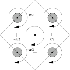
FIG. 1.: The order parameter in momentum space: $\Delta({\bf k})$ consists of four similarly oriented unit vortices around each Fermi point $(\pm\frac{\pi}{2},\pm\frac{\pi}{2})$. The phase of each vortex is relative to the direction of the ${\bf k}_{f}$ as in eq. (15). It changes the sign under $90^{o}$ rotation $\Delta(-k_{y},k_{x})=-\Delta(k_{x},k_{y})$.

8. Eq.(15) suggests an interesting generalization to the incommensurate case (optimal doping) where the Fermi surface is a simply connected curve rather than four Fermi pockets. We rewrite (14) approximately as

$$\Delta({\bf r})=\frac{e^{-i\arg({\bf r})}}{|{\bf r}|}\int dke^{i{\bf k}\cdot{\bf r}}e^{-i\arg({\bf k})}\Delta_{BCS}({\bf k})$$

Here ${\bf k}$ is relative to the center of the Brillouin zone and the factor $\arg({\bf k}_{\pm\pm})$ is replaced by $\arg({\bf k})$. It is possible, because $\Delta_{BCS}({\bf k})$ set the integral to the Fermi surface. At small doping it is shown in Fig.1. Away from half-filling $\epsilon_{\bf k}-\mu\sim v_{f}(|{\bf k}|-k_{f})$. Thus we obtain a ”tomographic” representation of the order parameter [15]:

$$\Delta({\bf k})=e^{-i2\arg({\bf k})}\int d{\bf k}_{f}\Delta_{BCS}({\bf k}-{\bf k}_{f}-{\bf q})D_{{\bf k}-{\bf k}_{f}}(q)d{\bf q}$$

where the propagator $D_{\bf p}({\bf q})=|{\bf q}|^{-1}\exp{(i\hat{{\bf p}{\bf q}})}$ is a holomorphic function of ${\bf q}$. Here $\hat{{\bf p}{\bf q}}$ is an angle between ${\bf p}$ and ${\bf q}$ and the integral $d{\bf k}_{f}$ goes over the Fermi surface.

This is the main result of this paper. It clarifies the physics of a topological superconductor. In contrast to BCS, an electron with momentum ${\bf k}$ close to ${\bf k}_{f}$ emits soft modes of density modulation with the propagator $D_{{\bf k}-{\bf k}_{f}}(q)$. As a result: (i) the ground states differing by an odd number of particles are orthogonal; (ii) the BCS wave function is dressed by soft density modes. This is analogous to 1D physics and bremsstrahlung of QED. The new features are: (i) emission of the soft mode is forward; (ii) the phase of the matrix element of the soft mode is the angle relative to the Fermi momentum.

9. Although the order parameter (15) forms a d-representation, its form and the physics behind it are drastically different from the conventional d-wave $\cos k_{x}-\cos k_{y}$. Nevertheless, it seems premature to speculate on an observable difference, until interlayer tunneling is taken into account. This is crucial, since the sign of parity breaking alternates between odd and even layers [16, 4], and a realistic junction averages over many layers. In a hypothetical monolayer tri-crystal experiment one would expect the trapped flux to be an integer (in contrast to half-integer for conventional d-wave [17]).

We would like to thank A. Larkin, K. Levin, B. Spivak and J. Talstra for numerous discussions and L. Radzihovsky for collaboration on the initial stage of this project. This work was supported by MRSEC NSF Grant DMR 9400379 and NSF Grant DMR 9509533. AGA also thanks Hulda B. Rotschild Fellowship for support.

REFERENCES

- [1] H. Fröhlich, Proc. R. Soc. A223, 296 (1954).
-
[2]
A. Fetter et.al., Phys. Rev. B 39, 9579 (1989);
Y.H. Chen et.al., Int.J.Mod.Phys. B3, 1001 (1989). - [3] P. Wiegmann, Progr. Theor. Phys. 107, 243 (1992).
- [4] P. Wiegmann in Field Theory, Topology, and condensed matter systems, ed. by H. Geyer (Springer 1995)
- [5] For related work see: D.S. Rokhsar, Phys. Rev. Lett. 70, 493 (1993); R.B.Laughlin, Physica C: 234, 280 (1994).
- [6] D.A. Wollman et.al., Phys. Rev. Lett. 71, 2134 (1993); For review see also J.Annett et.al. in Physical properties of high temperature superconductors, 5, D.M. Ginsberg (ed.), (World Scientific, Singapore, 1996).
- [7] A. Abanov, P. Wiegmann to be published
- [8] S. Chakravarty, P.W. Anderson, Phys. Rev. Lett. 72, 3859 (1994).
- [9] I. Affleck, J. Marston, Phys. Rev. B 37, 3774 (1988); X.-G. Wen et.al., ibid 39, 11413 (1989); R. Laughlin, Z. Zou, ibid 41, 664 (1989); D. Hasegawa et.al., Phys. Rev. Lett. 63, 907 (1989); P. Wiegmann, ibid 65, 2070 (1990).
- [10] D. Khveshchenko, P. Wiegmann, Phys. Rev. Lett. 73, 500 (1994).
- [11] For a more detailed discussion of validity of this and further approximations see [7].
- [12] Y. Aharonov, A. Casher, Phys. Rev. A 19, 2461 (1979).
- [13] For a related mechanism see S.M. Girvin et.al., Phys. Rev. Lett. 65, 1671 (1990).
- [14] Similar phenomenon has been discussed in 1D models: J.C. Talstra et.al., Phys. Rev. Lett. 74, 5256 (1995).
- [15] ”Tomographic” physics in electronic liquids was anticipated in A. Luther, Phys. Rev. B 19, 320, (1979), ibid. 50, 11446 (1994); P.W. Anderson, Phys. Rev. Lett. 64, 1839 (1990). .
- [16] R. Laughlin et.al., Nucl. Phys. B348, 693, (1991).
- [17] C.C. Tsuei et. al., Phys. Rev. Lett. 73, 593 (1994).