MATHEMATICAL THEORY OF THE WETTING
PHENOMENON IN THE 2D ISING MODEL$\,{}^{i}$

Abstract

We give a mathematical theory of the wetting phenomenon in the 2D Ising model using the formalism of Gibbs states. We treat the grand canonical and canonical ensembles.

Charles-Edouard Pfister

Département de Mathématiques, EPF-L
CH-1015 Lausanne, Switzerland
e-mail: cpfister@eldp.epfl.ch

and Yvan Velenik$\,{}^{ii}$

Département de Physique, EPF-L
CH-1015 Lausanne, Switzerland
e-mail:velenik@eldp.epfl.ch

1 Introduction

We study the wetting phenomenon in the 2D Ising model, starting from basic principles of Statistical Mechanics. The results of section 3 are based on [10], [11] and [12] and those of section 5 follow from recent results on the large deviations of the magnetization [26]. We shall in general refer to these papers for proofs. Our purpose is to give a global view of the mathematical results, which are now fairly complete. Since the results about large deviations are valid in the 2D case only we restrict the whole discussion to this case.

Let us suppose that we have a binary mixture and that the physical parameters are chosen so that we have coexistence of the two phases, called $+$ phase and $-$ phase. The system is inside a box; the horizontal bottom wall $w$ of the box adsorbs preferentially the $-$ phase. If we prepare the system in the $+$ phase we may observe the formation of a thin film of the $-$ phase between the wall $w$ and the $+$ phase in the bulk, so that the $+$ phase cannot be in contact with this wall. This is the phenomenon of complete wetting of the wall. Notice that the total amount of the $-$ phase is not fixed a priori. The appropriate statistical ensemble to describe this situation is a grand canonical ensemble. The surface tension $\widehat{\tau}(\theta)$ is the surface free energy due to an interface between the two coexisting phases, making an angle $\theta$ with an horizontal reference line. The contribution to the surface free energy due to the wall $w$ when the bulk phase is the $+$ phase is $\tau^{+}$. In the case of complete wetting of $w$ we expect that $\tau^{+}$ can be decomposed into $\tau^{-}+\widehat{\tau}(0)$, where $\tau^{-}$ is the surface free energy due to the wall $w$ in presence of the $-$ phase and $\widehat{\tau}(0)$ is the surface tension of an horizontal interface between the film of the $-$ phase and the bulk $+$ phase. On the other hand, if the wall adsorbs preferentially the $+$ phase, then we expect that

$$\tau^{+}=\tau^{-}-\widehat{\tau}(0)\,.$$ (1.1)

Indeed, if we impose the $-$ phase in the bulk, then we create an interface between the film of the $+$ phase near the wall and the $-$ bulk phase. When complete wetting does not occur a stability argument shows that one expects a strict inequality

$$|\tau^{+}-\tau^{-}|<\widehat{\tau}(0)\,.$$ (1.2)

In such a case the bulk phase is in contact with the wall. In other words the state of the system near the wall depends on the nature of the bulk phase. Therefore, depending on the property of the wall, we have

$$|\tau^{+}-\tau^{-}|\leq\widehat{\tau}(0)\,,$$ (1.3)

with equality if and only if complete wetting holds. This fundamental relation has been derived in a thermodynamical setting by Cahn [4]. In [10], [11] and [12] this situation is analysed in the Ising model and the fundamental inequality (1.3) is derived directly from the microscopic hamiltonian within the standard setting of Statistical Mechanics. The criterion for complete wetting,

$$|\tau^{+}-\tau^{-}|=\widehat{\tau}(0)\,,$$ (1.4)

is interpreted in terms of unicity of the (surface) Gibbs state.

It is possible to imagine another situation, which is often used to present the phenomenon of wetting of a wall. We have again the same system prepared in the $+$ phase, but we put a macroscopic droplet of the $-$ phase inside the box. The droplet is attached to the wall $w$ if the wall adsorbs preferentially the $-$ phase. The shape of the droplet depends on the interactions between the wall and the binary mixture; the shape of the droplet is given by the solution of an isoperimetric problem with constraint [29] (Winterbottom’s construction). Since the total amount of the $-$ phase is macroscopic and fixed, the relevant ensemble is a canonical ensemble. The case of complete wetting of the wall $w$ corresponds to the total spreading of the droplet of $-$ phase against the wall. The relation between the shape of the droplet and criterion (1.3) is made through the contact angle $\theta$ between the droplet and the wall (see Fig. 7),

$$\cos(\theta)\cdot\widehat{\tau}(\theta)-\sin(\theta)\cdot{d\widehat{\tau}(\theta)\over d\theta}=\tau^{+}-\tau^{-}\,,$$ (1.5)

the so–called Herring-Young equation. A derivation of (1.5) is given in section 4. Let us consider the following two extreme (degenerate) situations. When the wall adsorbs preferentially the $+$ phase, then

$$\tau^{+}-\tau^{-}=-\widehat{\tau}(0)<0\,.$$ (1.6)

This corresponds in (1.5) to $\theta=\pi$, which means that the droplet of $-$ phase is not attached to the wall. On the other hand, when the wall adsorbs preferentially the $-$ phase, then

$$\tau^{+}-\tau^{-}=\widehat{\tau}(0)>0\,,$$ (1.7)

which corresponds in (1.5) to the case $\theta=0$. This means that the droplet does not exist as such, but spreads out completely against the wall. We show that the above situations can be rigorously derived for the 2D Ising model in an appropriate canonical ensemble. The analysis consists in deriving sharp estimates of the large deviations of the magnetization [26]. Our work [26] extends considerably previous works [17], [18], [7], [24], [13] and [14] on the subject, since we can treat the case of an arbitrary boundary magnetic field.

2 Ising model

2.1 Gibbs states

The lattice is

$${{\mathchoice{\hbox{$\sf\textstyle Z\kern-3.99994ptZ$}}{\hbox{$\sf\textstyle Z\kern-3.99994ptZ$}}{\hbox{$\sf\scriptstyle Z\kern-2.10002ptZ$}}{\hbox{$\sf\scriptscriptstyle Z\kern-0.99998ptZ$}}}}^{2}:=\{\,t=(t(1),t(2)):\,t(i)\in{{\mathchoice{\hbox{$\sf\textstyle Z\kern-3.99994ptZ$}}{\hbox{$\sf\textstyle Z\kern-3.99994ptZ$}}{\hbox{$\sf\scriptstyle Z\kern-2.10002ptZ$}}{\hbox{$\sf\scriptscriptstyle Z\kern-0.99998ptZ$}}}}\,\}.$$ (2.1)

A spin configuration is a function $\omega$ defined on ${{\mathchoice{\hbox{$\sf\textstyle Z\kern-3.99994ptZ$}}{\hbox{$\sf\textstyle Z\kern-3.99994ptZ$}}{\hbox{$\sf\scriptstyle Z\kern-2.10002ptZ$}}{\hbox{$\sf\scriptscriptstyle Z\kern-0.99998ptZ$}}}}^{2}$, $t\mapsto\omega(t)$, with $\omega(t)=\pm 1$. The Ising variable at $t$ is

$$\sigma(t)(\omega):=\omega(t)\,.$$ (2.2)

An edge of ${{\mathchoice{\hbox{$\sf\textstyle Z\kern-3.99994ptZ$}}{\hbox{$\sf\textstyle Z\kern-3.99994ptZ$}}{\hbox{$\sf\scriptstyle Z\kern-2.10002ptZ$}}{\hbox{$\sf\scriptscriptstyle Z\kern-0.99998ptZ$}}}}^{2}$, ${{\langle t,t^{\prime}\rangle}}$, is a pair of nearest neighbours sites of the lattice ${{\mathchoice{\hbox{$\sf\textstyle Z\kern-3.99994ptZ$}}{\hbox{$\sf\textstyle Z\kern-3.99994ptZ$}}{\hbox{$\sf\scriptstyle Z\kern-2.10002ptZ$}}{\hbox{$\sf\scriptscriptstyle Z\kern-0.99998ptZ$}}}}^{2}$. We also call edge the unit–length segment in ${{\rm I\!R}}^{2}$ with end–points $t,t^{\prime}$. For each edge ${{\langle t,t^{\prime}\rangle}}$ we have a coupling constant $J({{\langle t,t^{\prime}\rangle}})\geq 0$. For each finite subset $\Lambda\subset{{\mathchoice{\hbox{$\sf\textstyle Z\kern-3.99994ptZ$}}{\hbox{$\sf\textstyle Z\kern-3.99994ptZ$}}{\hbox{$\sf\scriptstyle Z\kern-2.10002ptZ$}}{\hbox{$\sf\scriptscriptstyle Z\kern-0.99998ptZ$}}}}^{2}$ the energy is

$$H_{\Lambda}:=-\sum_{{{\langle t,t^{\prime}\rangle}}\cap\Lambda\not=\emptyset}J({{\langle t,t^{\prime}\rangle}})\sigma(t)\sigma(t^{\prime})\,.$$ (2.3)

Let $\omega^{*}$ be given; the Gibbs measure in $\Lambda$ with boundary condition $\omega^{*}$ and inverse temperature $\beta$ is the probability measure

$$\mu_{\Lambda}^{\omega^{*},\beta}(\omega):=\cases{Z^{\omega^{*}}(\Lambda)^{-1}\exp(-\beta H_{\Lambda}(\omega))&if $\omega(t)=\omega^{*}(t)$ for all $t\not\in\Lambda$\cr 0&otherwise.\cr}$$ (2.4)

The normalization constant is called partition function.

Assume that all coupling constants are equal to one. If we choose $\omega^{*}$ such that $\omega^{*}(t)=1$ for all $t$, then there is a limiting measure

$$\mu^{+,\beta}:=\lim_{\Lambda\uparrow{{\mathchoice{\hbox{$\sf\textstyle Z\kern-2.79996ptZ$}}{\hbox{$\sf\textstyle Z\kern-2.79996ptZ$}}{\hbox{$\sf\scriptstyle Z\kern-1.47002ptZ$}}{\hbox{$\sf\scriptscriptstyle Z\kern-0.69998ptZ$}}}}^{2}}\mu^{\omega^{*},\beta}_{\Lambda}\,.$$ (2.5)

The same is true for $\omega^{*}$, such that $\omega^{*}(t)=-1$ for all $t$. The limiting measure is $\mu^{-,\beta}$. These two Gibbs states are translation invariant and extremal. There is a unique Gibbs measure if and only if $\mu^{+,\beta}=\mu^{-,\beta}$. This happens if and only if $\beta\leq\beta_{c}$, where $\beta_{c}$ is the inverse critical temperature. The inverse critical temperature is characterized by the property that there is a positive spontaneous magnetization,

$$m^{*}(\beta):=\int\sigma_{t}(\omega)\mu^{+,\beta}(d\omega)>0$$ (2.6)

if and only if $\beta>\beta_{c}$.

2.2 Contours

Let $\omega^{*}$ be a fixed boundary condition. The usual way of describing the configurations of the model is to specify the pairs of nearest neighbours sites $e={{\langle t,t^{\prime}\rangle}}$ such that $\sigma(t)\sigma(t^{\prime})=-1$. Equivalently we specify the dual edges $e^{*}$, that is the edges of the dual lattice $({{\mathchoice{\hbox{$\sf\textstyle Z\kern-3.99994ptZ$}}{\hbox{$\sf\textstyle Z\kern-3.99994ptZ$}}{\hbox{$\sf\scriptstyle Z\kern-2.10002ptZ$}}{\hbox{$\sf\scriptscriptstyle Z\kern-0.99998ptZ$}}}}^{2})^{*}$,

$$({{\mathchoice{\hbox{$\sf\textstyle Z\kern-3.99994ptZ$}}{\hbox{$\sf\textstyle Z\kern-3.99994ptZ$}}{\hbox{$\sf\scriptstyle Z\kern-2.10002ptZ$}}{\hbox{$\sf\scriptscriptstyle Z\kern-0.99998ptZ$}}}}^{2})^{*}:=\{\,t=(t(1),t(2)):\,t(i)+1/2\in{{\mathchoice{\hbox{$\sf\textstyle Z\kern-3.99994ptZ$}}{\hbox{$\sf\textstyle Z\kern-3.99994ptZ$}}{\hbox{$\sf\scriptstyle Z\kern-2.10002ptZ$}}{\hbox{$\sf\scriptscriptstyle Z\kern-0.99998ptZ$}}}}\,\}$$ (2.7)

which cross the edges $e$. We decompose the set formed by all these dual edges into connected components. In [26] we further decompose the connected components into a set of paths, called ${\bf contours}$, using the rule given in Figure 1; for details see [26]. As set of edges the paths are disjoint two by two. Some paths are closed and are called closed contours; some are open and are called open contours.

Deformation rule

Figure 1: Two connected components giving rise to four contours

3 Grand canonical ensemble, Cahn’s criterion

3.1 Surface Gibbs states

Since we are interested in boundary effects, we consider the Ising model on the following rectangular box $\Lambda_{L}(r_{1},r_{2})=\Lambda_{L}$. Let $r_{1},r_{2}\in{{\rm I\!N}}$; we set

$$\Lambda_{L}(r_{1},r_{2}):=\{t\in{{\mathchoice{\hbox{$\sf\textstyle Z\kern-3.99994ptZ$}}{\hbox{$\sf\textstyle Z\kern-3.99994ptZ$}}{\hbox{$\sf\scriptstyle Z\kern-2.10002ptZ$}}{\hbox{$\sf\scriptscriptstyle Z\kern-0.99998ptZ$}}}}^{2}:\,-r_{1}L\leq t(1)<r_{1}L\,;\;0\leq t(2)<2r_{2}L\}\,.$$ (3.1)

The coupling constants of the model are

$$J({{\langle t,t^{\prime}\rangle}}):=\cases{h&if $t=(s,-1)$ and $t^{\prime}=(s,0)$ with $s\in{{\mathchoice{\hbox{$\sf\textstyle Z\kern-3.99994ptZ$}}{\hbox{$\sf\textstyle Z\kern-3.99994ptZ$}}{\hbox{$\sf\scriptstyle Z\kern-2.10002ptZ$}}{\hbox{$\sf\scriptscriptstyle Z\kern-0.99998ptZ$}}}}$,\cr 1&otherwise.\cr}$$ (3.2)

We consider four different boundary conditions

$$\omega^{*}(t):=\cases{a&$a=\pm 1$, if $t(2)<0$,\cr b&$b=\pm 1$, if $t(2)\geq 0$.\cr}$$ (3.3)

The hamiltonian $H_{L}\equiv H_{\Lambda_{L}}$ with $(a,b)$ boundary condition can be written

$$H_{L}=-\sum_{{\scriptstyle{{\langle t,t^{\prime}\rangle}}:\atop\scriptstyle t,t^{\prime}\in\Lambda_{L}}}\sigma(t)\sigma(t^{\prime})-\sum_{{\scriptstyle t\in\Lambda_{L}\,:\atop\scriptstyle t(2)=0}}ha\,\sigma(t)-\sum_{{\scriptstyle t\in\Lambda_{L}\,:t(2)=2r_{2}L\atop\scriptstyle{\rm or}\;t(1)=\pm r_{1}L}}b\,\sigma(t)\,.$$ (3.4)

The term

$$-\sum_{{\scriptstyle t\in\Lambda_{L}\,:\atop\scriptstyle t(2)=0}}ha\,\sigma(t)$$ (3.5)

describes the interaction of the binary mixture inside $\Lambda_{L}$ with the bottom wall of the box $\Lambda_{L}$, which plays the role of the wall $w$. The wall adsorbs preferentially the $a$ phase. We interpret $ha$ as a real–valued boundary magnetic field and we refer to the $b$–part of the boundary condition,

$$-\sum_{{\scriptstyle t\in\Lambda_{L}\,:t(2)=2r_{2}L\atop\scriptstyle{\rm or}\;t(1)=\pm r_{1}L}}b\,\sigma(t)\,,$$ (3.6)

as the boundary condition. Expectation value with respect to the Gibbs measure in $\Lambda_{L}$ is denoted by ${{\langle\,\cdot\,\rangle}}_{L}^{b}(\beta,h)$. When $h\geq 0$ and $b=1$, then all contours of a configuration are closed. On the other hand, when $h<0$ and $b=1$, then there is exactly one open contour in each configuration, denoted below by $\lambda$, with end–points $t_{l,L}=(-r_{1}L-1/2,-1/2)$ and $t_{r,L}=(r_{1}L-1/2,-1/2)$. The boundary condition (3.6) specifies the type $b$ of the phase in the bulk of the system in the following sense . Let $\beta>\beta_{c}$ and $\delta>0$. Given $\varepsilon>0$ there exist $L_{0}$ and $d$ such that, $\forall L\geq L_{0}$,

$$|{{\langle\sigma(t)\rangle}}_{L}^{+}(\beta,h)-m^{*}(\beta)\,|\leq\varepsilon\,,$$ (3.7)

for all $t=(t(1),t(2))\in\Lambda_{L}$ satisfying the conditions

$$|t(1)-r_{1}L|\geq d\quad,\quad|t(2)-2r_{2}L|\geq d\quad,\quad t(2)\geq L^{1/2+\delta}\,.$$ (3.8)

The surface Gibbs states are the limiting measures

$${{\langle\,\cdot\,\rangle}}^{b}(\beta,h):=\lim_{L\rightarrow\infty}{{\langle\,\cdot\,\rangle}}_{L}^{b}(\beta,h)\,,$$ (3.9)

or limiting measures defined by choosing different boundary conditions. The existence of the limits when $b=\pm$, as well as the following properties are proven in [10].

1. The two states ${{\langle\,\cdot\,\rangle}}^{b}(\beta,h)$, $b=\pm$, are extremal Gibbs states.

2. They are invariant under the translations $x\mapsto x+y$, $y=(y(1),0)$.

3. There is a unique surface Gibbs measure if and only if ${{\langle\,\cdot\,\rangle}}^{+}(\beta,h)={{\langle\,\cdot\,\rangle}}^{-}(\beta,h)$.

3.2 Surface tension and surface free energies

We define the basic thermodynamic quantities which enter in the description of the wetting phenomenon. More details on the surface tension are given in [23] and [24] section 6. Surface free energies are studied in [10] and [11]; see also [26]. The definitions we use are standard. Explanations for them are given in [23]. These definitions are not very satisfactory from a conceptual point of view (see beginning of the introduction of [2]), since they are defined without using a precise notion of interface. This weak point is also a strong point, because the notion of interface is a delicate notion, which is difficult to analyse.

3.2.1 Surface tension

For latter purposes (see section 4) it is more convenient to parametrize surface tension using the normal vector to the interface instead of the angle $\theta$. We consider the model with coupling constants equal to one on the whole lattice. Let $\Omega_{L}$ be the square box

$$\Omega_{L}:=\{t\in{{\mathchoice{\hbox{$\sf\textstyle Z\kern-3.99994ptZ$}}{\hbox{$\sf\textstyle Z\kern-3.99994ptZ$}}{\hbox{$\sf\scriptstyle Z\kern-2.10002ptZ$}}{\hbox{$\sf\scriptscriptstyle Z\kern-0.99998ptZ$}}}}^{2}:\,-L\leq t(1),t(2)\leq L\}\,.$$ (3.10)

Let $n=(n(1),n(2))$ be a unit vector in ${{\rm I\!R}}^{2}$ and ${\cal L}(n)$ a line perpendicular to $n$, passing through $(0,0)$. We define a boundary condition $\omega^{n}$ by setting (see Fig. 2)

$$\omega^{n}(t):=\cases{1&if $t$ is above or on the line ${\cal L}(n)$,\cr-1&if $t$ is below the line ${\cal L}(n)$.\cr}$$ (3.11)

The corresponding partition function is $Z^{\omega^{n}}(\Omega_{L})$. By definition, the surface tension of an interface perpendicular to $n$ is

$$\widehat{\tau}(n):=\lim_{L\rightarrow\infty}-{1\over 2L}\ln{Z^{\omega^{n}}(\Omega_{L})\over Z^{+}(\Omega_{L})}\,.$$ (3.12)

$\Omega_{L}$$n$${\cal L}(n)$

Figure 2: Definition of the $\omega^{n}$ boundary condition

We usually do not write explicitly the $\beta$–dependence of the surface tension. We extend the function $\widehat{\tau}$ to ${{\rm I\!R}}^{2}$ as a positively homogeneous function. By GKS–inequalities it follows that the function is subadditive,

$$\widehat{\tau}(x+y)\leq\widehat{\tau}(x)+\widehat{\tau}(y)\,.$$ (3.13)

It can be shown that $\widehat{\tau}$ is strictly positive (for all $x\not=0$) if and only if $\beta>\beta_{c}$ [16]. (This is also true for dimensions higher than two.)

Remark: In dimension two the surface tension is related by duality to the decay–rate of the two–point function at the dual inverse temperature [3], [24]. The decay–rate of the two–point function at the dual inverse temperature can be computed explicitly [19]. The surface tension has the following symmetry properties,

$$\widehat{\tau}(n)=\widehat{\tau}(-n)\quad{\rm and}\quad\widehat{\tau}(n)=\widehat{\tau}(m)\quad{\rm if}\quad n\perp m\,.$$ (3.14)

It is a smooth function for any $\beta<\infty$.

3.2.2 Surface free energies

The coupling constants are given by (3.2). Free energies are defined up to an arbitrary constant. We need only to define $\tau^{-}-\tau^{+}$, the difference of the contributions of the wall $w$ to the free energy, when the bulk phase is the $-$ phase respectively the $+$ phase. The definition is similar to the definition of the surface tension. Let $\Lambda_{L}$ be the box (3.1). By definition,

$$\tau^{-}-\tau^{+}:=\lim_{L\rightarrow\infty}-{1\over 2r_{1}L}\ln{Z^{-}(\Lambda_{L})\over Z^{+}(\Lambda_{L})}\,.$$ (3.15)

We usually do not write explicitly the $(\beta,h)$–dependence of $\tau^{-}-\tau^{+}$. The existence of the limit is proven in [11], as well as the following results.

1. For any $\beta$, $|\tau^{-}-\tau^{+}|\leq\widehat{\tau}((1,0))$. Hence $\tau^{-}-\tau^{+}=0$ for all $\beta\leq\beta_{c}$.

2. We have the symmetry

   $$\tau^{-}(h)-\tau^{+}(h)=-\Big{(}\tau^{-}(-h)-\tau^{+}(-h)\Big{)}\,.$$ (3.16)

3. Let $\beta>\beta_{c}$ and $n_{w}:=(0,-1)$. For positive $h$, $\tau^{-}(h)-\tau^{+}(h)$ is a positive concave function; for all $h\geq 1$

   $$\tau^{-}(h)-\tau^{+}(h)=\widehat{\tau}(n_{w})\,.$$ (3.17)

These results are not restricted to dimension two.

Remark: In dimension two the quantity $\tau^{-}-\tau^{+}$ can be computed [22]. For $h$ positive it is equal to the decay–rate of the boundary two–point function at the dual coupling constants.

3.3 Cahn’s criterion and phase diagram

In all the section the inverse critical temperature $\beta>\beta_{c}$ is fixed. We study the model in the grand canonical ensemble; the coupling constants are given by (3.2) and the states are the surface Gibbs states ${{\langle\,\cdot\,\rangle}}^{b}$ of subsection 3.1. For definiteness we choose the $+$ boundary condition, so that we have the $+$ phase as bulk phase.

From the properties of $\tau^{-}-\tau^{+}$, which are stated in subsection 3.2.2, we have the existence of a positive $h^{*}(\beta)$ such that (see Fig. 3)

$$h^{*}(\beta):=\inf\Big{\{}h\geq 0:\,\tau^{-}(\beta,h)-\tau^{+}(\beta,h)=\widehat{\tau}(n_{w})(\beta)\Big{\}}\,.$$ (3.18)

The thermodynamical criterion of Cahn states that there is complete wetting of the wall if and only if $|h|\geq h^{*}(\beta)$.

$\tau^{-}-\tau^{+}$$h$$h^{*}$$1$$\widehat{\tau}(n_{w})$

Figure 3: $\tau^{-}-\tau^{+}$ as a function of $h$.

Remark: The value of $h^{*}(\beta)$ is known in dimension two. It was computed by Abraham [1]; $h^{*}(\beta)$ is the solution of the equation

$$\exp\{2\beta\}\{\cosh 2\beta-\cosh 2\beta h^{*}(\beta)\}=\sinh 2\beta\,.$$ (3.19)

In [12], see also [25], it is shown that the value of $h^{*}(\beta)$ can also be obtained from the work of McCoy and Wu [19].

To make the connection with the surface Gibbs states we use the identity proven in [11]

$$\tau^{-}(\beta,h)-\tau^{+}(\beta,h)=\int_{0}^{h}\Big{(}{{\langle\sigma(0)\rangle}}^{+}(\beta,h^{\prime})-{{\langle\sigma(0)\rangle}}^{-}(\beta,h^{\prime})\Big{)}\,dh^{\prime}\,.$$ (3.20)

Therefore

$$\widehat{\tau}(n_{w}) = \tau^{-}(\beta,h^{*})-\tau^{+}(\beta,h^{*})$$

$$= \int_{0}^{h^{*}}\Big{(}{{\langle\sigma(0)\rangle}}^{+}(\beta,h^{\prime})-{{\langle\sigma(0)\rangle}}^{-}(\beta,h^{\prime})\Big{)}\,dh^{\prime}\,.$$

For all $h\geq h^{*}$ we must have

$${{\langle\sigma(0)\rangle}}^{+}(\beta,h)={{\langle\sigma(0)\rangle}}^{-}(\beta,h)\,,$$ (3.22)

since for positive $h^{\prime}$

$${{\langle\sigma(0)\rangle}}^{+}(\beta,h^{\prime})\geq{{\langle\sigma(0)\rangle}}^{-}(\beta,h^{\prime})\,.$$ (3.23)

On the other hand, if $0\leq h<h^{*}$, the concavity of $\tau^{-}(\beta,h)-\tau^{+}(\beta,h)$ as function of $h$ implies that

$${{\langle\sigma(0)\rangle}}^{+}(\beta,h)>{{\langle\sigma(0)\rangle}}^{-}(\beta,h)\,.$$ (3.24)

These results, together with the properties of the surface Gibbs states mentionned in subsection 3.1, imply the following interpretation of the Cahn’s criterion for complete wetting (see also the corresponding phase diagram of Fig. 4).

1. There is complete wetting of the wall $w$ if and only if there is a unique surface Gibbs state.

2. There is a unique surface Gibbs state if and only if

   $$|\tau^{-}(\beta,h)-\tau^{+}(\beta,h)|=\widehat{\tau}(n_{w})(\beta)>0\,.$$ (3.25)

3. The value $h^{*}$ of the boundary magnetic field where the wetting transition takes place can be defined as

   $$h^{*}(\beta):=\inf_{h\geq 0}\Big{\{}{{\langle\,\cdot\,\rangle}}^{+}(\beta,h)={{\langle\,\cdot\,\rangle}}^{-}(\beta,h)\Big{\}}\,.$$ (3.26)

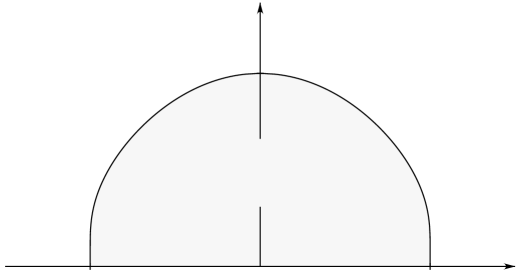
$T$$T_{c}$$h$$1$$-1$Non-uniqueness ofsurface Gibbs state

Figure 4: Phase diagram. The region of non-uniqueness of the surface Gibbs state is shaded. In the other region, there is a single surface Gibbs state.

Remarks: 1. These results are proven in [11]; they are not restricted to dimension two.

2. In dimension two we have precise information about the behaviour of the open contour $\lambda$ entering in the description of the configurations when we have $-$ boundary condition and $0\leq h<h^{*}$. The contours sticks to the wall. There exists a constant $K$, such that the probability that the open contour $\lambda$ does not visit the segment $I=\{t:\,t(2)=0,x_{1}\leq t(1)\leq x_{2}\}$ is smaller than

$$K\exp\{-\kappa\cdot|x_{1}-x_{2}|\}\,,$$ (3.27)

with

$$\kappa=\widehat{\tau}(n_{w})-\Big{(}\tau^{-}-\tau^{+}\Big{)}\,.$$ (3.28)

This result is a combination of Lemma 7.1 in [26] and the remark following the proof of that lemma. By symmetry the same result applies to the case where we have $+$ boundary condition and $0\geq h>-h^{*}$.

3. Weaker results about the behaviour of $\lambda$, but not restricted to dimension two, are contained in [11].

4 Variational problem

We consider here the variational problem giving the shape of the macroscopic droplet when the surface tension and the surface free energies of the wall are known. In section 5 we show how this variational problem arises when the analysis starts from the hamiltonian of the model.

The variational problem, which gives the shape of the macroscopic droplet in presence of a wall, is a generalization of the classical isoperimetric problem. In the physics literature the solution of the problem is known as Winterbottom’s construction [29]. Wulff’s construction [30] corresponds to the special case when the wall has no effect on the droplet. Dinghas [5] gave a geometrical proof of Wulff’s construction, which has been extended by Taylor (see her review [28] for original references). Wulff’s solution and Bonnesen’s inequalities, which describe a (strong) stability property of the solution, are discussed in details in [7]. A completely different proof, valid in the 2D case only, is given in [6]. The many facets of statistical mechanics of equilibrium shapes are reviewed in [27] and [31].

4.1 Geometry of the boundary of a convex body

Let $C\subset{{\rm I\!R}}^{2}$ be a compact convex body, that is, a compact convex set with a non–empty interior. We denote by $\partial C$ the boundary of $C$ and by $(x|y)$ the Euclidean scalar product of $x,y\in{{\rm I\!R}}^{2}$. The support function of $C$, $\tau_{C}$, is defined on ${{\rm I\!R}}^{2}$ by

$$\tau_{C}(y):=\sup_{x\in C}(x|y)\,.$$ (4.1)

It is immediate from the definition (4.1) that $\tau_{C}$ is positively homogeneous and subadditive,

$$\tau_{C}(y_{1}+y_{2})\leq\tau_{C}(y_{1})+\tau_{C}(y_{2})\,.$$ (4.2)

Since $C$ is compact it is also clear that for any $y$ there exists $x_{y}\in C$, in fact $x_{y}\in\partial C$, with

$$\tau_{C}(y)=(x_{y}|y)\,.$$ (4.3)

Let $n\in{{\rm I\!R}}^{2}$ be of norm $\|n\|=1$. Define $A(n)$ to be the hyperplane

$$A(n):=\{x\in{{\rm I\!R}}^{2}:\,(x|n)=\tau_{C}(n)\}\,.$$ (4.4)

Then $A(n)$ is a support plane for $C$ at $x_{n}$, that is $x_{n}\in A(n)$ and

$$C\subset\{x\in{{\rm I\!R}}^{2}:\,(x|n)\leq\tau_{C}(n)\}\,.$$ (4.5)

Conversely, if $x\in\partial C$, then there exists a support plane for $C$ at $x$. This is a consequence of the separation result: if $O$ is an open convex set and $L$ an affine subset, such that $O\cap L=\emptyset$, then there exists a hyperplane $H$ with the properties [8]

$$L\subset H\quad{\rm and}\quad O\cap H=\emptyset\,.$$ (4.6)

For $n\in{{\rm I\!R}}^{2}$, $\|n\|=1$, $\tau_{C}(n)$ gives the (signed) distance of the hyperplane $A(n)$ to the origin. The distance is positive if and only if $0\in\{x\in{{\rm I\!R}}^{2}:\,(x|n)\leq\tau_{C}(n)\}$.

Theorem 4.1

Let $C$ be a compact convex body in ${{\rm I\!R}}^{2}$. Let $\tau_{C}$ be its support function. Then

$$C = \{x\in{{\rm I\!R}}^{2}:\,(x|n)\leq\tau_{C}(n)\;\forall n\,,\|n\|=1\}$$

$$= \bigcap_{n:\,\|n\|=1}\{x\in{{\rm I\!R}}^{2}:\,(x|n)\leq\tau_{C}(n)\}\,.$$

Proof. It is clear that

$$C\subset\bigcap_{n:\,\|n\|=1}\{x\in{{\rm I\!R}}^{2}:\,(x|n)\leq\tau_{C}(n)\}\,.$$ (4.8)

Suppose that $y\not\in C$. We can separate strictly a closed convex set $B$ and a compact convex set $K$ by a hyperplane, when they are disjoint [8]. Therefore there exists a hyperplane

$$H=\{x\in{{\rm I\!R}}^{2}:\,(x|m)=\delta\}\,,$$ (4.9)

$\|m\|=1$, such that for all $x\in C$ we have $(x|m)<\delta$ and at the same time $(y|m)>\delta$. Therefore

$$\sup_{x\in C}(x|m)=\tau_{C}(m)\leq\delta\,,$$ (4.10)

and consequently

$$y\not\in\bigcap_{n:\,\|n\|=1}\{x\in{{\rm I\!R}}^{2}:\,(x|n)\leq\tau_{C}(n)\}\,.$$ (4.11)

$\sqcap$$\sqcup$

We recall two definitions (see Fig. 5). A point $y\in\partial C$ is a regular point if there is a single support plane containing $y$. This is equivalent to say that the intersection of all support planes containing $y$ is a $1$–dimensional affine set. At a regular point $x$ there is a well–defined (unit) normal vector to $C$, defined as the vector $n$ such that $x\in A(n)$. A support plane $A$ is a regular support plane if $A\cap C$ is $0$–dimensional.

Theorem 4.2

Let $C$ be a compact convex body. Let $n\in{{\rm I\!R}}^{2}$, $\|n\|=1$. Then $A(n)\cap C$ coincides with the subdifferential $\partial\tau_{C}(n)$ of $\tau_{C}$ at $n$, that is,

$$A(n)\cap C=\{x\in{{\rm I\!R}}^{2}:\,\tau_{C}(z+n)\geq\tau_{C}(n)+(z|x)\quad\forall z\in{{\rm I\!R}}^{2}\}\,.$$ (4.12)

Proof. Suppose that $x\in\partial\tau_{C}(n)$,

$$\tau_{C}(z+n)\geq\tau_{C}(n)+(z|x)\;\forall z\in{{\rm I\!R}}^{2}\,.$$ (4.13)

Since $\tau_{C}$ is subadditive,

$$\tau_{C}(z)+\tau_{C}(n)\geq\tau_{C}(n)+(z|x)\,,$$ (4.14)

we have

$$\tau_{C}(z)\geq(z|x)\quad\forall z\,;$$ (4.15)

hence $x\in C$ by Theorem 4.1. On the other hand,

$$(z+n|x)-\tau_{C}(z+n)\leq(n|x)-\tau_{C}(n)\,;$$ (4.16)

therefore

$$\tau^{*}_{C}(x)=\sup_{y\in{{\rm I\!R}}^{2}}\Big{\{}\,(y|x)-\tau_{C}(y)\,\Big{\}}=(n|x)-\tau_{C}(n)\,.$$ (4.17)

Since $x\in C$, we have for all $y$

$$(y|x)-\tau_{C}(y)\leq 0\,;$$ (4.18)

hence

$$\sup_{y\in{{\rm I\!R}}^{2}}\Big{\{}\,(y|x)-\tau_{C}(y)\,\Big{\}}=0\,,$$ (4.19)

that is $x\in A(n)$.

Conversely, suppose that $x\in A(n)\cap C$. Since $x\in A(n)$ we have

$$(x|n)=\tau_{C}(n)\,.$$ (4.20)

Since $x\in C$ we have for all $z$

$$\tau_{C}(z+n)\geq(z+n|x)\,.$$ (4.21)

Therefore

$$\tau_{C}(z+n)\geq(n|x)+(z|n)=\tau_{C}(n)+(z|n)\,.$$ (4.22)

$\sqcap$$\sqcup$

$C$$O$$x_{1}$$x_{2}$$y_{1}$$y_{2}$grad$\tau(n_{2})$$n_{1}$$n_{2}$$P_{1}$$P_{2}$$A(n_{1})$$A(n_{2})$

Figure 5: Convex body $C$ with support planes $A(n_{1})$, $A(n_{2})$. $x_{2}$ is a regular point and $A(n_{2})$ is a regular support plane. $x_{1}$ is a regular point and $A(n_{1})$ is not regular. The vectors $y_{1}$ and $y_{2}$ are in the subdifferential of $\tau$ at $n_{1}$. dist$(O,P_{1})=\tau(n_{1})$; dist$(O,P_{2})=\tau(n_{2})$.

As a consequence of Theorem 4.2 the support plane $A(n)$ is regular if and only if $\tau_{C}$ is differentiable at $n$, $\|n\|=1$. On the other hand the regular points of $\partial C$ are characterized by the points of $\partial C$ where the normal is well–defined (there is a unique tangent plane at those points). We can partition the boundary $\partial C$ of $C$ into three sets.

1. $x$ is regular and the support plane $A(n)$, $n$ the unit normal vector to $C$ at $x$, is regular. The support function $\tau_{C}$ is differentiable at $n$.

2. $x$ is regular and the support plane $A(n)$, $n$ the unit normal vector to $C$ at $x$, is not regular. The support function $\tau_{C}$ is not differentiable at $n$. The facet of (unit) normal $n$ is given by the subdifferential of the support function $\tau_{C}$ at $n$,

   $$A(n)\cap C=\partial\tau_{C}\,.$$ (4.23)

3. $x$ is not regular. Such a point corresponds to a corner of $C$, where the normal is not well–defined. There are at least two different support planes.

Remarks: 1. The dual function of $\tau_{C}$ is

$$\tau_{C}^{*}(x):=\sup_{y\in{{\rm I\!R}}^{2}}\Big{\{}\,(x|y)-\tau_{C}(y)\,\Big{\}}\,.$$ (4.24)

In our case the dual function $\tau_{C}^{*}$ is the indicator function of $C$:

$$\tau_{C}^{*}(x)=\cases{0&if $x\in C$,\cr\infty&if $x\not\in C$.\cr}$$ (4.25)

(See proof of Theorem 4.2.) The dual function of $\tau_{C}^{*}$ is $\tau_{C}$,

$$\tau_{C}^{**}(x):=\sup_{y\in{{\rm I\!R}}^{2}}\Big{\{}\,(x|y)-\tau_{C}^{*}(y)\,\Big{\}}=\tau_{C}(x)\,.$$ (4.26)

2. There is another interesting function associated to $C$, the polar of $C$, $\tau_{C}^{\circ}$,

$$\tau_{C}^{\circ}(x):=\sup_{n\in{{\rm I\!R}}^{2}\,\|n\|=1}{(x|n)\over\tau_{C}(n)}\,.$$ (4.27)

The convex body $C$ can be expressed as

$$C=\Big{\{}x\in{{\rm I\!R}}^{2}:\,\tau_{C}^{\circ}(x)\leq 1\Big{\}}\,,$$ (4.28)

and its boundary as

$$\partial C=\Big{\{}x\in{{\rm I\!R}}^{2}:\,\tau_{C}^{\circ}(x)=1\Big{\}}\,.$$ (4.29)

A point of $\partial C$ is regular if and only if $\tau_{C}^{\circ}$ is differentiable at $x$.

4.2 Isoperimetric inequality

Let $C$ be a compact convex body in ${{\rm I\!R}}^{2}$ and $\tau_{C}$ its support function. Let $\partial V$ be a rectifiable curve in ${{\rm I\!R}}^{2}$, which is the boundary of an open set $V$. The curve $\partial V$ is oriented in the usual way; $n(x)$ denotes the exterior unit normal vector at a point $x\in\partial V$. We define a functional

$${\cal F}_{C}(\partial V):=\int_{\partial V}\,\tau_{C}(n(s))ds\,.$$ (4.30)

If $\gamma:[0,t]\rightarrow{{\rm I\!R}}^{2}$ is a parametrization of the boundary $\partial V$, then, using the homogeneity property of $\tau_{C}$, we can write the functional as

$${\cal F}_{C}(\partial V):=\int_{0}^{t}\,\tau_{C}\Big{(}(\dot{\gamma}(2)(u),-\dot{\gamma}(1)(u))\Big{)}du\,,$$ (4.31)

where $\dot{\gamma}(s)$ is the derivative of $\gamma$ with respect to $s$. The functional is always positive. Indeed, by a suitable translation $a$ we can suppose that the translated set $C^{\prime}=C+a$ has zero as interior point, and consequently its support function $\tau_{C^{\prime}}$ is strictly positive at $x\not=0$. Since

$$\tau_{C^{\prime}}(x)=\tau_{C}(x)+(x|a)\,,$$ (4.32)

and

$$\int_{\partial V}\,(n(s)|a)ds=0\,,$$ (4.33)

the value of the functional does not depend on $a$.

Theorem 4.3 (Generalized isoperimetric inequality)

Let $C$ be a compact convex body in ${{\rm I\!R}}^{2}$. Let $V$ be an open set in ${{\rm I\!R}}^{2}$ such that its boundary is a rectifiable curve $\partial V$. The Lebesgue measure of $C$ and $V$ is denoted by $|C|$ and $|V|$. Then

$${\cal F}_{C}(\partial V)\geq 2|C|^{1/2}|V|^{1/2}\,.$$ (4.34)

Equality holds in (4.34) if and only if $V$ equals, up to dilation and translation, the set $C$.

Remarks: 1. The set $V$ may have several connected components.

2. The main ingredient of Dinghas’ proof [5] is to express the functional $\tau_{C}$ in a geometrical manner as

$${\cal F}_{C}(\partial V)=\lim_{\varepsilon\downarrow 0}{|V+\varepsilon C|-|V|\over\varepsilon}\,,$$ (4.35)

where $V+\varepsilon C$ denotes the set

$$\bigcup_{x\in V}\,(x+\varepsilon C)\,,$$ (4.36)

and $\varepsilon C=\{\varepsilon x:\,x\in C\}$. The isoperimetric inequality follows by applying Brunn-Minkowski inequality to $V+\varepsilon C$,

$$|V+\varepsilon C|^{1/2}\geq|V|^{1/2}+|\varepsilon C|^{1/2}\,.$$ (4.37)

3. When $C$ is the unit ball we recover the classical isoperimetric inequality.

4. The minimum of the functional for open sets $V$ with $|V|=|C|$ can easily be computed,

$$\min_{V:\,|V|=|C|}{\cal F}_{C}(\partial V)=2\cdot|C|\,.$$ (4.38)

In addition to the isoperimetric inequality, the stability of the minimum can be controlled in a rather strong sense by the (generalized) Bonnesen’s inequalities. Let

$$r(\partial V)=\sup\Big{\{}r:\,r\cdot C+x\subset V\;\hbox{for some $x\in{{\rm I\!R}}^{2}$}\Big{\}}$$ (4.39)

and

$$R(\partial V)=\inf\Big{\{}R:\,R\cdot C+x\supset V\;\hbox{for some $x\in{{\rm I\!R}}^{2}$}\Big{\}}\,.$$ (4.40)

Then

$${{\cal F}_{C}(\partial V)-\Bigl{[}{\cal F}_{C}(\partial V)^{2}-4|C|\cdot|V|\Bigr{]}^{1/2}\over 2|C|} \leq r(\partial V)\leq R(\partial V)$$

$$\leq {{\cal F}_{C}(\partial V)+\Bigl{[}{\cal F}_{C}(\partial V)^{2}-4|C|\cdot|V|\Bigr{]}^{1/2}\over 2|C|}\,.$$

4.3 Variational problem

Let $r_{1},r_{2}\in{{\rm I\!N}}$ be given and define the rectangle $Q$,

$$Q:=\{x=(x(1),x(2))\in{{\rm I\!R}}^{2}:\,-r_{1}\leq x(1)\leq r_{1}\,;\,0\leq x(2)\leq 2r_{2}\}\,.$$ (4.42)

Let $\beta>\beta_{c}$ and $\widehat{\tau}:{{\rm I\!R}}^{2}\rightarrow{{\rm I\!R}}$ be the surface tension. Let $S^{1}=\{n\in{{\rm I\!R}}^{2}:\,\|n\|=1\}$; we define on $Q\times S^{1}$ a function ${\tt t}$,

$${\tt t}(x;n):=\cases{\tau^{-}-\tau^{+}&if $x(2)=0$ and $n=n_{w}$,\cr\widehat{\tau}(n)&otherwise.\cr}$$ (4.43)

We define a functional as above, by setting

$${\tt W}_{{\tt t}}(\partial V):=\int_{\partial V}\,{\tt t}(s;n(s))\,ds\,.$$ (4.44)

Notice that $\tau^{-}-\tau^{+}$ is negative when $h$ is negative. However, as long as $\tau^{-}-\tau^{+}>-\widehat{\tau}(n_{w})$, then the functional is positive. This is an easy consequence of the elementary monotonicity principle stated in subsection 4.3.1.

Let us give the interpretation of ${\tt W}_{{\tt t}}(\gamma)$ in our setting. We consider a macroscopic droplet of the $-$ phase immersed in the $+$ phase. The boundary of the droplet is $\partial V$. Suppose first that $x(2)\not=0$ and $\|n\|=1$. Then ${\tt t}(x;n)$ is interpreted as the surface tension of an interface perpendicular to $n$, passing through $x$. The case $x(2)=0$ and $n=n_{w}$ corresponds to the situation where the macroscopic droplet is in contact with the wall. In that case

$$\tau^{-}-\tau^{+}$$ (4.45)

is the change in the free energy due to the presence of the droplet on the wall (the bulk phase is the $+$ phase).

Variational problem VP: Suppose that the bulk phase in $Q$ is the $+$ phase and that the $-$ phase occupies a set $V$ such that $|V|$ is a fraction $\alpha$ of the volume of $Q$, $|V|=\alpha|Q|$. $V$ is not necessarily connected, but we assume that it is open and that its boundary $\partial V$ is a rectifiable curve. Find the optimal set $C$, $|C|=\alpha|Q|$, such that $C$ minimizes the functional ${\tt W}_{{\tt t}}(\partial V)$, $|V|=\alpha|Q|$.

Remarks: 1. In [26] we consider the same variational problem. Its formulation is slightly different, because we have introduced as fundamental quantities the dual quantities, the decay–rates of the two–point functions.

2. There is a simple way of showing that the solution $C$ is a convex body. Let us consider the case where ${\tt t}(x,n)=\widehat{\tau}(n)$. Since $\widehat{\tau}$ is convex and positively homogeneous, we have for any parametrized curve $\gamma:\,[a,b]\rightarrow{{\rm I\!R}}^{2}$, by Jensen’s inequality

$${1\over b-a}\int_{a}^{b}\widehat{\tau}\Big{(}(\dot{\gamma}(2)(s),-\dot{\gamma}(1)(s))\Big{)}ds\geq$$ (4.46)

$$\widehat{\tau}\Bigl{(}\Bigl{(}{\gamma(2)(b)-\gamma(2)(a)\over b-a},-{\gamma(1)(b)-\gamma(1)(a)\over b-a}\Bigr{)}\Bigr{)}\,.$$

Therefore one decreases the value of the functional each time we replace some part of the curve between two points by the straight segment between these two points. Since the box $Q$ is convex, for every open set $V\subset Q$ its convex enveloppe ${\rm conv}\,V\subset Q$, and $|{\rm conv}\,V|\geq|V|$. On the other hand

$${\tt W}_{{\tt t}}(\partial V)\geq{\tt W}_{{\tt t}}\Big{(}\partial({\rm conv}\,V)\Big{)}\,.$$ (4.47)

4.3.1 Solution of the variational problem

We give the explicit solution in some special cases. We refer to [15] for other cases. We consider cases where only the effect of the bottom horizontal wall is important. This amounts to consider cases where the amount of $-$ phase is not too large. (Theorem 5.1 is valid without such restrictions.)

The function $\widehat{\tau}$ can be interpreted as the support function of a compact convex set, which we denote by $C_{\widehat{\tau}}$,

$$C_{\widehat{\tau}}:=\Big{\{}x\in{{\rm I\!R}}^{2}:\,(x|y)\leq\widehat{\tau}(y)\;\forall y\Big{\}}\,.$$ (4.48)

Indeed, the dual function $\widehat{\tau}^{*}$ is the indicator function of the set $C_{\widehat{\tau}}$, so that the support function of $C_{\widehat{\tau}}$, which the dual of the indicator function is $\widehat{\tau}^{**}=\widehat{\tau}$, because $\widehat{\tau}$ is convex. The compact convex body $C_{\widehat{\tau}}$ is called Wulff shape in the physics literature.

Case 1: $\tau^{-}-\tau^{+}=\widehat{\tau}(n_{w})$.

In that case ${\tt t}$ is independent of the variable $x$, so that

$${\tt t}(x,n)=\widehat{\tau}(n)\,.$$ (4.49)

Let us fix the volume of the set $V$ occupied by the $-$ phase to be $\alpha|Q|$, $0<\alpha<1$. Ignoring for a moment the constraint that $V\subset Q$, the solution of the variational problem is given by Theorem 4.3. It is a Wulff shape of volume $\alpha|Q|$, $\lambda\cdot C_{\widehat{\tau}}$, with

$$\lambda={\alpha|Q|\over|C_{\widehat{\tau}}|}\,.$$ (4.50)

Whenever a translate of $\lambda\cdot C_{\widehat{\tau}}$ can be put inside $Q$, this is a solution of the variational problem. When there is no translate of $\lambda\cdot C_{\widehat{\tau}}$ which can be put inside $Q$, then the constraint that $V\subset Q$ modifies the shape of the optimal set $V$ (see [15]).

Case 2: $|\tau^{-}-\tau^{+}|<\widehat{\tau}(n_{w})$.

Let us first ignore the constraint that $V\subset Q$. Notice that the problem without the constraint $V\subset Q$ is scale–invariant. Then the solution is given by a Winterbottom shape of volume $\alpha|Q|$. The Winterbottom shape is by definition the convex body (see Fig. 6)

$$C_{{\tt t}}:=\widehat{C}\cap\{x:\,(x|n_{w})\leq\tau^{-}-\tau^{+}\}\,.$$ (4.51)

$O$$n_{w}$$\tau^{-}-\tau^{+}$

Figure 6: Winterbottom construction.

To prove the optimality of the Winterbottom shape we use Theorem 4.3 and the following monotonicity principle [15]. Suppose that we can find a convex body $C$, such that the following two conditions (4.52) and (4.53) are verified. If we replace in the definition of the functional ${\tt W}_{{\tt t}}$ the function ${\tt t}$ by the support function $\tau_{C}$, then

$${\tt W}_{{\tt t}}(\partial V)\geq{\tt W}_{\tau_{C}}(\partial V)\,,$$ (4.52)

and for $V=C$,

$${\tt W}_{{\tt t}}(\partial C)={\tt W}_{\tau_{C}}(\partial C)\,.$$ (4.53)

Then we have

$${\tt W}_{{\tt t}}(\partial V)\geq 2|C|^{1/2}|V|^{1/2}$$ (4.54)

and

$${{\tt W}_{{\tt t}}(\partial V)-\Bigl{[}{\tt W}_{{\tt t}}(\partial V)^{2}-4|C|\cdot|V|\Bigr{]}^{1/2}\over 2|C|} \leq r(\partial V)\leq R(\partial V)$$

$$\leq {{\tt W}_{{\tt t}}(\partial V)+\Bigl{[}{\tt W}_{{\tt t}}(\partial V)^{2}-4|C|\cdot|V|\Bigr{]}^{1/2}\over 2|C|}\,.$$

The proof of (4.54) is an immediate consequence of Theorem 4.3 applied to the convex set $C$. The proof of (4.3.1) is an immediate consequence of the monotonicity of the real function

$$s\mapsto s-(s^{2}-D)^{1/2}$$ (4.56)

for $|s|\geq\sqrt{D}$. In our case $C=C_{{\tt t}}$. It is immediate that condition (4.53) is verified. To show (4.52) we notice that ${\tt t}^{*}$ is the indicator function of $C_{{\tt t}}$. Therefore its support function satisfies

$${\tt t}(n)\geq{\tt t}^{**}(n)=\tau_{C}(n)\,.$$ (4.57)

Any translate of the Winterbottom shape, which is contained in $Q$, is a solution of the variational problem. When there is no translate which is inside $Q$, then the constraint that $V\subset Q$ effectively modifies the shape of the optimal set $V$. We want to discuss one simple situation of that kind (see Fig. 8 and 9 for illustrations). Suppose that $\alpha$ is chosen so that a translate of the Winterbottom shape of volume $\alpha|Q|$ exists inside $Q$ whenever $h\geq 0$. Let $h(\alpha)$ be the smallest value of $h$ such that a translate of the Winterbottom shape of volume $\alpha|Q|$ exists inside $Q$. Notice that necessarily $h(\alpha)>-h^{*}$, and that the value of $h(\alpha)$ is a function of the box $Q$. Then for any $h\leq h(\alpha)$ the solution of the problem is the same as the solution of the problem for $h=h(\alpha)$: the box prevents the macroscopic droplet to spread out. For $h\leq h(\alpha)$ the optimal shape of the droplet of volume $\alpha|Q|$ is not the corresponding Winterbottom shape.

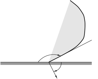
$-\varphi$$n$$\theta$

Figure 7: Angles $\theta$ and $\varphi$

Remark: The Young–Herring relation, giving the contact angle $\theta$ of the macroscopic droplet with the wall in terms of the surface tension and surface free energies, can be easily derived from Theorem 4.2. Let us parametrize the unit vectors in ${{\rm I\!R}}^{2}$ by an angle $\varphi$ as in figure 7. Let $n$ be the normal to the interface defining the contact angle $\theta$. Theorem 4.2 asserts that

$${\rm grad}\widehat{\tau}(n)(2)=-(\tau^{-}-\tau^{+})\,.$$ (4.58)

This is exactly Young–Herring relation. Indeed, in polar coordinates the surface tension is

$$\widehat{\tau}(r,\varphi):=r\cdot\widehat{\tau}(n(\varphi))\,,$$ (4.59)

so that, using $x(2)=r\sin\varphi$ and $\varphi+\theta=\pi/2$, we get ($\widehat{\tau}(1,\varphi)\equiv\widehat{\tau}(\varphi)$)

$${\rm grad}\widehat{\tau}(n)(2) = \sin\varphi\,\widehat{\tau}(\varphi)+\cos\varphi\,{d\over d\varphi}\widehat{\tau}(\varphi)$$

$$= \cos\theta\,\widehat{\tau}(\theta)-\sin\theta\,{d\over d\theta}\widehat{\tau}(\theta)$$

$$= -(\tau^{-}-\tau^{+})\,.$$

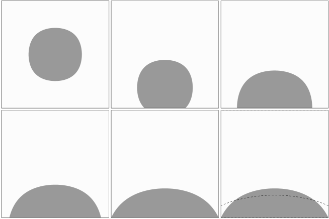
abcdef

Figure 8: a: $h>h^{*}$; b: $0<h<h^{*}$; c: $h=0$; d, e, f: a sequence of droplets for decreasing values of $-h^{*}<h<0$. The droplet spreads until it begins to touch the vertical sides of the box (e). Further reduction of the magnetic field does not modify the shape of the droplet, but makes it unstable in the sense that the removal of the vertical walls would result in a spreading of the droplet. f: the dashed line shows only a part of the droplet which would be obtained by removing the walls when $0>h>-h^{*}$.

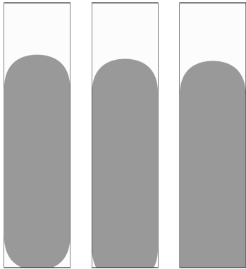
abc

Figure 9: Sequence of big droplets in a tube for decreasing value of the magnetic field. a,b: The upper part of the droplet has the Wulff shape, while the lower part has the winterbottom shape; they are joined by a rectangle such that the total volume is conserved; c: The droplet completely wets the lower wall, the droplet is build up from a half Wulff shape and a rectangle. This situation holds as long as $-h^{*}<h\leq 0$.

5 Canonical ensemble and macroscopic droplet

To study the macroscopic droplet of fixed volume we introduce a canonical ensemble. There is some freedom in doing this, in the sense that we can fix the total magnetization up to fluctuations, which are negligible when measured at the scale of the volume. In subsection 5.1 we define the canonical states and in subsection 5.2 we consider the limit of the lattice spacing going to zero. We show that in this limit there is a droplet of the $-$ phase immersed in the $+$ phase and that the shape of the droplet is given by the variational problem of subsection 4.3. This completes the mathematical theory of wetting in the 2D Ising model in terms of the Gibbs states. We always consider the case of $+$ boundary condition.

5.1 Canonical states

We define the canonical states at finite volume. Let $\beta>\beta_{c}$ and $-m^{*}<m<m^{*}$. Let $c=1/4-\delta>0$, with $\delta>0$. We introduce the event

$$A(m;c):=\{\omega:\,|\,\sum_{t\in\Lambda_{L}}\omega(t)-m|\Lambda_{L}|\,|\leq|\Lambda_{L}|\cdot L^{-c}\}\,.$$ (5.1)

The canonical state in $\Lambda$, with $+$ boundary condition and parameter $m$, is the conditional state

$${{\langle\,\cdot\,|\,m\rangle}}_{L}^{+}(\beta,h):={{\langle\,\cdot\,|\,A(m;c)\rangle}}_{L}^{+}(\beta,h)\,.$$ (5.2)

To understand the canonical state (5.2) we must control the large deviations of the magnetization in the state ${{\langle\,\cdot\,\rangle}}^{+}_{L}$. Although for typical set of configurations with respect to ${{\langle\,\cdot\,\rangle}}_{L}^{+}$ the length of the contours is small , because we impose here a specific magnetization $m\not=m^{*}$ there is always at least one large contour in each typical set of configurations of the canonical state. It is therefore natural to distinguish between large and small contours. Let $B(0;[L^{\delta}])$ be the square box

$$B(0;[L^{\delta}]):=\{t\in{{\rm I\!R}}^{2}:\,|t(j)|\leq[L^{\delta}]\;,\;j=1,2\}\,.$$ (5.3)

We say that a contour $\gamma$ is small if there exits a translate of the box $B(0;[L^{\delta}])$ which contains $\gamma$. Otherwise the contour is ${\bf large}$. We sum over small contours and the large contours are treated by a coarse–graining method. Theorems 11.1 and 11.2 in [26] give a detailled description of a set of typical configurations in terms of large contours. One result of this analysis is the exact computation of the large deviations of the magnetization for the Gibbs state ${{\langle\,\cdot\,\rangle}}_{L}^{+}(\beta,h)$, together with a control of the speed of convergence.

Theorem 5.1

Assume that $\beta>\beta_{c}$, $h\in{{\rm I\!R}}$, $-m^{*}(\beta)<m<m^{*}(\beta)$ and $c:=1/4-\delta$, $\delta>0$. Let ${\tt W}^{*}_{{\tt t}}(m)$ be defined by

$${\tt W}^{*}_{{\tt t}}(m):=\inf\Big{\{}{\tt W}_{{\tt t}}({\cal C}):\,{\cal C}\subset Q\,,\,{\rm vol\,}{\cal C}={m^{*}-m\over 2m^{*}}|Q|\Big{\}}\,.$$ (5.4)

Then for any $\eta<\delta$ and $L$ large enough

$$|\,{1\over L}\ln P_{L}^{{\rm h}}[A(m;c)]+{\tt W}^{*}_{{\tt t}}(m)\,|\leq O(L^{\eta-\delta})\,;$$ (5.5)

the probability is computed with the measure ${{\langle\,\cdot\,\rangle}}_{L}^{+}(\beta,h)$.

5.2 Macroscopic droplet

In this last subsection we consider the limit of the lattice spacing going to zero. We suppose that $\beta>\beta_{c}$, $h\in{{\rm I\!R}}$ and we choose the $+$ boundary condition. The probability measure in this section is always the canonical Gibbs state ${{\langle\,\cdot\,|m\rangle}}_{L}^{+}(\beta,h)$ defined in subsection 5.1 with $-m^{*}<m<m^{*}$ and $c=1/4-\delta>0$ fixed. We do the analysis in the box $\Lambda_{L}(r_{1},r_{2})$ and at the end we scale everything by $1/L$, i.e. we take the limit of the lattice spacing going to zero.

Let $C\subset{{\mathchoice{\hbox{$\sf\textstyle Z\kern-3.99994ptZ$}}{\hbox{$\sf\textstyle Z\kern-3.99994ptZ$}}{\hbox{$\sf\scriptstyle Z\kern-2.10002ptZ$}}{\hbox{$\sf\scriptscriptstyle Z\kern-0.99998ptZ$}}}}^{2}$; the empirical magnetization in $C$ is

$$m_{C}(\omega):={1\over|C|}\sum_{t\in C}\sigma(t)(\omega)\,.$$ (5.6)

Let $0<a<1$; we introduce a grid ${\cal L}(a)$ in $\Lambda_{L}$ made of cells which are translates of the square box

$$B(0;[L^{a}])=\{t\in{{\rm I\!R}}^{2}:\,|t(j)|\leq[L^{a}]\;,\;j=1,2\}\,.$$ (5.7)

The value of $a$ is close to $1$. In most of the cells the empirical magnetization is close to $m^{*}$ or $-m^{*}$ with high probability. For each cell of the grid ${\cal L}(a)$ we compute the empirical magnetization $m_{C}(\omega)$. Then we scale all lengths by $1/L$, so that after scaling the box $\Lambda_{L}$ is the rectangle $Q$. For each $\omega$ we define a magnetization profile $\rho_{L}(x;\omega)$ on $Q$,

$$\rho_{L}(x;\omega):=m_{C}(\omega)\;\hbox{if $Lx\in C$}\,$$ (5.8)

where $Lx$ is the point $x\in Q$ scaled by $L$ and $C$ a cell of the grid ${\cal L}(a)$.
The set of macroscopic droplets at equilibrium is

$${\cal D}(m):=\{\,{\cal V}\subset Q:\,|{\cal V}|={m^{*}-m\over 2m^{*}}|Q|\,,\,{\tt W}_{{\tt t}}(\partial{\cal V})={\tt W}_{{\tt t}}^{*}(m)\,\}\,.$$ (5.9)

For each ${\cal V}\in{\cal D}(m)$ we have a magnetization profile,

$$\rho_{{\cal V}}(x):=\cases{m^{*}&if $x\in Q\backslash{\cal V}$,\cr-m^{*}&$x\in{\cal V}$.\cr}$$ (5.10)

Let $f$ be a real–valued function on $Q$; we set

$$d_{1}(f,{\cal D}(m)):=\inf_{{\cal V}\in{\cal D}(m)}\int_{Q}dx\,|\,f(x)-\rho_{{\cal V}}(x)\,|\,.$$ (5.11)

The main theorem (Theorem 12.2 in [26]) is

Theorem 5.2

Let $\beta>\beta_{c}$, $h\in{{\rm I\!R}}$, $-m^{*}<m<m^{*}$, $c=1/4-\delta>0$. Let ${{\langle\,\cdot\,|\,m\,\rangle}}_{L}^{+}(\beta,h)$ be the canonical Gibbs state with $+$ boundary condition. Then there exists a positive function $\overline{\varepsilon}(L)$ such that $\lim_{L\rightarrow\infty}\overline{\varepsilon}(L)=0$ and for $L$ large enough

$${\rm Prob}[\,\{\,d_{1}(\rho_{L}(\,\cdot\,;\omega),{\cal D}(m))\leq\overline{\varepsilon}(L)\,\}\,]\geq 1-\exp\{-O(L^{\kappa})\}\,.$$ (5.12)

This theorem gives a complete description of the wetting phenomenon in the canonical state, making the connection between a microscopic approach with a conditional state and the macroscopic variational problem giving the shape of a macroscopic droplet at equilibrium. The two approaches with grand canonical and canonical ensembles give of course the same information about the occurence of the wetting transition. However, for this surface phenomenon they are not equivalent, but complementary.

References

• [1] Abraham D.B.: Solvable model with a roughening transition for a planar Ising ferromagnet Phys. Rev. Lett. 44, 1165–1168 (1980).
• [2] Alberti G., Bellettini G., Cassandro M., Presutti E.: Surface tension in Ising systems with Kac potentials to appear in J. Stat. Phys. (1996).
• [3] Bricmont J., Lebowitz J.L., Pfister C.-E.: On the surface tension of lattice systems. Annals of the New York Academy of Sciences 337, 214–223 (1980).
• [4] Cahn J.W.: Critical point wetting J. Chem. Phys. 66, 3667-3672 (1977).
• [5] Dinghas A.: Uber einen geometrischen Satz von Wulff fur die Gleichtgewichtsform von Kristallen. Zeitschrift fur Kristallographie 105, 301–314 (1944).
• [6] Dacorogna B., Pfister C.-E.: Wulff theorem and best constant in Sobolev inequality. J. Math. Pures Appl. 71 97–118 (1992).
• [7] Dobrushin R.L., Kotecký R., Shlosman S.: Wulff construction: a global shape from local interaction. AMS translations series (1992).
• [8] Eggleston Convexity Cambridge University Press, Cambridge (1977).
• [9] Fonseca I.: The Wulff theorem revisited Proc.R.Soc. Lond. A 432, 125–145 (1991).
• [10] Fröhlich J., Pfister C.-E.: Semi–infinite Ising model I. Thermodynamic functions and phase diagram in absence of magnetic field. Commun. Math. Phys. 109, 493–523 (1987).
• [11] Fröhlich J., Pfister C.-E.: Semi–infinite Ising model II. The wetting and layering transitions. Commun. Math. Phys. 112, 51–74 (1987).
• [12] Fröhlich J., Pfister C.-E.: The wetting and layering transitions in the half–infinite Ising model. Europhys. Lett. 3, 845–852 (1987).
• [13] Ioffe D.: Large deviations for the 2D Ising model: a lower bound without cluster expansions. J. Stat. Phys. 74 411–432 (1994).
• [14] Ioffe D.: Exact large deviation bounds up to $T_{c}$ for the Ising model in two dimensions. Prob. Th. Rel. Fields. 102 313–330 (1995).
• [15] Kotecký R., Pfister C.-E.: Equilibrium shapes of crystals attached to walls. J. Stat. Phys. 76, 419-445 (1994).
• [16] Lebowitz J.L., Pfister C.-E.: Surface tension and phase coexistence. Phys. Rev. Lett. 46, 1031–1033 (1981).
• [17] Minlos R.A., Sinai Ya.G.: The phenomenon of phase separation at low temperatures in some lattice models of a gas I. Math. USSR– Sbornik 2, 335–395 (1967).
• [18] Minlos R.A., Sinai Ya.G.: The phenomenon of phase separation at low temperatures in some lattice models of a gas II. Trans. Moscow Math. Soc. 19, 121–196 (1968).
• [19] McCoy B.M., Wu T.T.: The Two–dimensional Ising Model. Harvard University Press, Cambridge, Massachusetts (1973).
• [20] Osserman R.: The isoperimetric inequality Amer. Math. Soc. 84, 1182–1238 (1978).
• [21] Osserman R.: Bonnesen-style isoperimetric inequalities Amer. Math. Monthly 86, 1–29 (1979).
• [22] Patrick A.: private communication (1996).
• [23] Pfister C.-E.: Interface and surface tension in Ising model. In Scaling and self–similarity in physics. ed. J. Fröhlich, Birkhäuser, Basel, pp. 139–161 (1983).
• [24] Pfister C.-E.: Large deviations and phase separation in the two–dimensional Ising model. Helv. Phys. Acta 64, 953–1054 (1991).
• [25] Pfister C.-E., Penrose O.: Analyticity properties of the surface free energy of the Ising model Commun. Math. Phys. 115, 691–699 (1988).
• [26] Pfister C.-E., Velenik Y.: Large deviations and boundary effects for the 2D Ising model. Preprint (1996). To appear in Prob. Th. Rel. Fields.
• [27] Rotman C., Wortis M.: Statistical mechanics of equilibrium crystal shapes: Interfacial phase diagrams and phase transitions Phys. Rep. 103, 59–79 (1984).
• [28] Taylor J.E.: Some crystalline variational techniques and results Astérisque 154-155, 307–320 (1987).
• [29] Winterbottom W.L.: Equilibrium shape of a small particle in contact with a foreign substrate Acta Metallurgica 15, 303–310 (1967).
• [30] Wulff G.: Zur Frage der Geschwindigkeit des Wachstums and der Auflösung der Kristallflächen. Zeitschrift fur Kristallographie 34, 449-530 (1901).
• [31] Zia R.K.P.: Anisotropic surface tension and equilibrium crystal shapes in Progress in Statistical Physics, C.K. Hu, ed., World Scinetific, Singapore (1988), 303–357.