Quantum Computation with Quantum Dots

Abstract

We propose a new implementation of a universal set of one- and two-qubit gates for quantum computation using the spin states of coupled single-electron quantum dots. Desired operations are effected by the gating of the tunneling barrier between neighboring dots. Several measures of the gate quality are computed within a newly derived spin master equation incorporating decoherence caused by a prototypical magnetic environment. Dot-array experiments which would provide an initial demonstration of the desired non-equilibrium spin dynamics are proposed.

I Introduction

The work of the last several years has greatly clarified both the theoretical potential and the experimental challenges of quantum computation[1]. In a quantum computer the state of each bit is permitted to be any quantum-mechanical state of a qubit (two-level quantum system). Computation proceeds by a succession of “two-qubit quantum gates”[2], coherent interactions involving specific pairs of qubits, by analogy to the realization of ordinary digital computation as a succession of boolean logic gates. It is now understood that the time evolution of an arbitrary quantum state is intrinsically more powerful computationally than the evolution of a digital logic state (the quantum computation can be viewed as a coherent superposition of digital computations proceeding in parallel).

Shor has shown[3] how this parallelism may be exploited to develop polynomial-time quantum algorithms for computational problems, such as prime factoring, which have previously been viewed as intractable. This has sparked investigations into the feasibility of the actual physical implementation of quantum computation. Achieving the conditions for quantum computation is extremely demanding, requiring precision control of Hamiltonian operations on well-defined two-level quantum systems, and a very high degree of quantum coherence[4]. In ion-trap systems[5], and in cavity quantum electrodynamic experiments[6], quantum computation at the level of an individual two-qubit gate has been demonstrated; however, it is unclear whether such atomic-physics implementations could ever be scaled up to do truly large-scale quantum computation, and some have speculated that solid-state physics, the scientific mainstay of digital computation, would ultimately provide a suitable arena for quantum computation as well. The initial realization of the model that we introduce here would correspond to only a modest step towards the realization of quantum computing, but it would at the same time be a very ambitious advance in the study of controlled non-equilibrium spin dynamics of magnetic nanosystems, and could point the way towards more extensive studies to explore the large-scale quantum dynamics envisioned for a quantum computer.

II Quantum-dot implementation of two-qubit gates

In this report we develop a detailed scenario for how quantum computation may be achieved in a coupled quantum dot system[7]. In our model the qubit is realized as the spin of the excess electron on a single-electron quantum dot, see Fig. 1. We introduce here a novel mechanism for two-qubit quantum-gate operation that operates by a purely electrical gating of the tunneling barrier between neighboring quantum dots, rather than by spectroscopic manipulation as in other models. Controlled gating of the tunneling barrier between neighboring single-electron quantum dots in patterned two-dimensional electron-gas structures has already been achieved experimentally using a split-gate technique[8]. If the barrier potential is “high”, tunneling is forbidden between dots, and the qubit states are held stably without evolution in time ($t$). If the barrier is pulsed to a “low” voltage, the usual physics of the Hubbard model[9] says that the spins will be subject to a transient Heisenberg coupling,

$$H_{s}(t)=J(t)\vec{S}_{1}\cdot\vec{S}_{2}\,\,,$$ (1)

where $J(t)=\frac{4t_{0}^{2}(t)}{u}$ is the time-dependent exchange constant[10] which is produced by the turning on and off of the tunneling matrix element $t_{0}(t)$. Here $u$ is the charging energy of a single dot, and $\vec{S}_{i}$ is the spin-1/2 operator for dot $i$.

Eq. (1) will provide a good description of the quantum-dot system if several conditions are met: 1) Higher-lying single particle states of the dots can be ignored; this requires $\Delta E\gg kT$, where $\Delta E$ is the level spacing and $T$ is the temperature. 2) The time scale $\tau_{s}$ for pulsing the gate potential “low” should be longer than $\hbar/\Delta E$, in order to prevent transitions to higher orbital levels. 3) $u>t_{0}(t)$ for all $t$; this is required for the Heisenberg-exchange approximation to be accurate. 4) The decoherence time $\Gamma^{-1}$ should be much longer than the switching time $\tau_{s}$. Much of the remainder of the paper will be devoted to a detailed analysis of the effect of a decohering environment. We expect that the spin-1/2 degrees of freedom in quantum dots should generically have longer decoherence times than charge degrees of freedom, since they are insensitive to any environmental fluctuations of the electric potential. However, while charge transport in such coupled quantum dots has received much recent attention[11, 8] we are not aware of investigations on their non-equilibrium spin dynamics as envisaged here. Thus, we will carefully consider the effect of magnetic coupling to the environment.

If $\Gamma^{-1}$ is long, then the ideal of quantum computing may be achieved, wherein the effect of the pulsed Hamiltonian is to apply a particular unitary time evolution operator $U_{s}(t)=T\exp\{-i\int_{0}^{t}H_{s}(t^{\prime})dt^{\prime}\}$ to the initial state of the two spins: $|\Psi(t)\rangle=U_{s}|\Psi(0)\rangle$. The pulsed Heisenberg coupling leads to a special form for $U_{s}$: For a specific duration $\tau_{s}$ of the spin-spin coupling such that $\int dtJ(t)=J_{0}\tau_{s}=\pi$ (mod $2\pi$)[12], $U_{s}(J_{0}\tau_{s}=\pi)=U_{sw}$ is the “swap” operator: if $|ij\rangle$ labels the basis states of two spins in the $S_{z}$-basis with $i,j=0,1$, then $U_{sw}|ij\rangle=|ji\rangle$. Because it conserves the total angular momentum of the system, $U_{sw}$ is not by itself sufficient to perform useful quantum computations, but if the interaction is pulsed on for just half the duration, the resulting “square root of swap” is very useful as a fundamental quantum gate: for instance, a quantum XOR gate is obtained by a simple sequence of operations:

$$U_{XOR}=e^{i{\pi\over 2}S_{1}^{z}}e^{-i{\pi\over 2}S_{2}^{z}}U_{sw}^{\frac{1}{2}}e^{i\pi S_{1}^{z}}U_{sw}^{\frac{1}{2}}\,\,,$$ (2)

where $e^{i\pi S_{1}^{z}}$ etc. are single-qubit operations only, which can be realized e.g. by applying local magnetic fields (see Sec. III B) [13]. It has been established that XOR along with single-qubit operations may be assembled to do any quantum computation[2]. Note that the XOR of Eq. (2) is given in the basis where it has the form of a conditional phase-shift operation; the standard XOR is obtained by a simple basis change for qubit 2[2].

III The master equation

We will now consider in detail the non-ideal action of the swap operation when the two spins are coupled to a magnetic environment. A new master equation model is obtained that explicitly accounts for the action of the environment during switching — to our knowledge, the first treatment of this effect. We use a Caldeira-Leggett type model in which a set of harmonic oscillators are coupled linearly to the system spins by $H_{int}=\lambda\sum_{i=1,2}\vec{S}_{i}\cdot\vec{b}_{i}$. Here, $b_{i}^{j}=\sum_{\alpha}g^{ij}_{\alpha}(a_{\alpha,ij}+a_{\alpha,ij}^{\dagger})$ is a fluctuating quantum field whose free motion is governed by the harmonic oscillator Hamiltonian $H_{B}=\sum\omega_{\alpha}^{ij}a_{\alpha,ij}^{\dagger}a_{\alpha,ij}$, where $a_{\alpha,ij}^{\dagger}$/$a_{\alpha,ij}$ are bosonic creation/annihilation operators (with $j=x,y,z$), and $\omega_{\alpha}^{ij}$ are the corresponding frequencies with spectral distribution function $J_{ij}(\omega)=\pi\sum_{\alpha}(g^{ij}_{\alpha})^{2}\delta(\omega-\omega_{\alpha})$[14]. The system and environment are initially uncorrelated with the latter in thermal equilibrium described by the canonical density matrix $\rho_{B}$ with temperature $T$. We assume for simplicity that the environment acts isotropically and is equal and independent on both dots. We do not consider this to be a microscopically accurate model for these as-yet-unconstructed quantum dot systems, but rather as a generic phenomenological description of the environment of a spin, which will permit us to explore the complete time dependence of the gate action on the single coupling constant $\lambda$ and the controlled parameters of $H_{s}(t)$[15].

A Swap gate

The quantity of interest is the system density matrix $\rho(t)=Tr_{B}{\bar{\rho}}(t)$ which we obtain by tracing out the environment degrees of freedom. The full density matrix ${\bar{\rho}}$ itself obeys the von Neumann equation,

$$\dot{\bar{\rho}}(t)=-i[H,{\bar{\rho}}]\equiv-i{\cal L}{\bar{\rho}},$$ (3)

where

$${\cal L}={\cal L}_{s}(t)+{\cal L}_{int}+{\cal L}_{B}$$ (4)

denotes the Liouvillian[16] corresponding to the full Hamiltonian

$$H=H_{s}(t)+H_{int}+H_{B}.$$ (5)

Our goal is to find the linear map (superoperator) ${\cal V}(t)$ which connects the input state of the gate $\rho_{0}=\rho(t=0)$ with the output state $\rho(t)$ after time $t>\tau_{s}$ has elapsed, $\rho(t)={\cal V}(t)\,\rho_{0}\,.\$ ${\cal V}(t)$ must satisfy three physical conditions: 1) trace preservation $Tr_{s}\,{\cal V}\rho=1$, where $Tr_{s}$ denotes the system trace, 2) Hermiticity preservation $({\cal V}\rho)^{\dagger}={\cal V}\rho$, and 3) complete positivity, $({\cal V}\otimes 1_{B})\bar{\rho}\geq 0$. Using the Zwanzig master equation approach [16] we sketch the derivation for ${\cal V}$ in the Born and Markov approximation which respects these three conditions. The novel situation we analyze here is unusual in that $H_{s}$ is explicitly time-dependent and changes abruptly in time. It is this fact that requires a separate treatment for times $t\leq\tau_{s}$ and $t>\tau_{s}$. To implement this time scale separation and to preserve positivity it is best to start from the exact master equation in pure integral form,

$$\rho(t)={\cal U}_{s}(t,0)\rho_{0}-\!\int_{0}^{t}\!d\sigma\int_{0}^{\sigma}\!d\tau{\cal U}_{s}(t,\sigma){\cal M}(\sigma,\tau)\rho(\tau),$$ (6)

where

$${\cal U}_{i}(t,t^{\prime})=T\exp\{-i\int_{t^{\prime}}^{t}d\tau{\cal L}_{i}(\tau)\},$$ (7)

where $i=s,\ B,\ int,\ {\rm or}\ q$. Here $q$ indicates the projected Liouvillian

$${\cal L}_{q}=(1-P){\cal L}=(1-\rho_{B}Tr_{B}){\cal L}.$$ (8)

Also, the “memory kernel” is

$${\cal M}(\sigma,\tau)=Tr_{B}{\cal L}_{int}{\cal U}_{q}(\sigma,\tau){\cal L}_{int}\rho_{B}.$$ (9)

We solve (6) in the Born approximation and for $t\gg\tau_{s}$. To this end the time integrals are split up into three parts, 1) $0\leq\tau\leq\sigma\leq\tau_{s}<t$, 2) $0\leq\tau\leq\tau_{s}\leq\sigma<t$, and 3) $0\leq\tau_{s}\leq\tau\leq\sigma<t$. Keeping only leading terms in $\tau_{s}$ we retain the contribution from interval 2) as it is proportional to $\tau_{s}$, whereas we can drop interval 1) which leads to higher-order terms. But note that terms containing $J_{0}\tau_{s}$ must be kept to all orders [12]. Interval 3) is independent of $\tau_{s}$.

Rewriting the expressions and performing a Born approximation (i.e., keeping only lowest order terms in $\lambda^{2}$) with subsequent Markov approximation we find, for $t\geq\tau_{s}$,

$${\cal V}(t)=e^{-(t-\tau_{s}){\cal K}_{3}}{\cal U}_{s}(\tau_{s})\,(1-{\cal K}_{2})\,\,,$$ (10)

where ${\cal U}_{i}(\tau_{s})={\cal U}_{i}(\tau_{s},0)$, ${\cal K}_{2}$ describes the effect of the environment during the switching,

$${\cal K}_{2}= {\cal U} {}_{s}^{\dagger}(\tau_{s})\int_{0}^{\tau_{s}}d\tau\int_{0}^{\infty}dt\$$ (11)

$$\times Tr_{B}{\cal L}_{int}{\cal U}_{s}(\tau){\cal U}_{B}(t){\cal L}_{int}\rho_{B}{\cal U}_{s}(\tau_{s}-\tau),$$ (12)

while

$${\cal K}_{3}=\int_{0}^{\infty}dt\ Tr_{B}\ {\cal L}_{int}{\cal U}_{B}(t){\cal L}_{int}\rho_{B}$$ (13)

is independent of $H_{s}$. We also note that ${\cal U}_{s}(1-{\cal K}_{2})$ has a simple interpretation as being the “transient contribution” which changes the initial value $\rho_{0}$ at $t=0$ to ${\cal U}_{s}(\tau_{s})(1-{\cal K}_{2})\rho_{0}$ at $t=\tau_{s}$. We show in the Appendix that, to leading order, our superoperator $\cal V$ indeed satisfies all three conditions stated above, in particular complete positivity. Such a proof for spins with an explicit time-dependent and direct interaction, Eq. (1), is not simply related to the case of a master equation for non-interacting spins (and without explicit time-dependence) considered in the literature (see for example [17, 16]). We also note that the above Born and Markov approximations could also be introduced in the master equation in the more usual differential-integral representation. However, it is well-known from studies in non-interacting spin problems[18] that in this case the resulting propagator is in general no longer completely positive.

Next, we evaluate the above superoperators more explicitly, obtaining

$${\cal K}_{2}\rho = (\Gamma+i\Delta)\sum_{i}\int_{0}^{\tau_{s}}d\tau[\vec{S}_{i}(\tau_{s}),\cdot\vec{S}_{i}(\tau)\rho]+h.c.\,\,,$$ (14)

$${\cal K}_{3}\rho = \Gamma(3\rho-2\sum_{i}\vec{S}_{i}\rho\cdot\vec{S}_{i})\,\,,$$ (15)

where $\Gamma,\Delta$ are real and given by

$$\Gamma = {\lambda^{2}\over\pi}\int_{0}^{\infty}dt\int_{0}^{\infty}d\omega J(\omega)\cos(\omega t)\coth({\omega\over 2k_{B}T})\,,$$ (16)

$$\Delta = {\lambda^{2}\over\pi}\int_{0}^{\infty}dt\int_{0}^{\infty}d\omega J(\omega)\sin(\omega t)\,.$$ (17)

In our model, the transverse and longitudinal relaxation or decoherence rates of the system spins are the same and given by $\Gamma$. For instance, for ohmic damping with $J(\omega)=\eta\omega$, we get $\Gamma=\lambda^{2}\eta k_{B}T$ and $\Delta=\lambda^{2}\eta\omega_{c}/\pi$, with $\omega_{c}$ some high frequency cut-off. Requiring for consistency that $\Gamma\tau_{s},\Delta\tau_{s}\ll 1$ we find that ${\cal K}_{2}$ is in fact a small correction. However, we emphasize again that, to our knowledge, this is the first time that any analysis of this ${\cal K}_{2}$ term, describing the action of the environment during the finite time that the system Hamiltonian is switched on, has been given.

For further evaluation of ${\cal V}$ we adopt a matrix representation, defined by

$${\cal V}_{ab|cd}=(e_{ab},{\cal V}e_{cd})\equiv Tr_{s}e_{ab}^{\dagger}{\cal V}e_{cd},$$ (18)

where $\{e_{ab}|a,b=1,..,4\}$ is an orthonormal basis, i.e. $(e_{ab},e_{cd})=\delta_{ac}\delta_{bd}$. In this notation we then have

$$\rho(t)_{ab}=\sum_{c,d}{\cal V}_{ab|cd}(\rho_{0})_{cd}$$ (19)

with ${\cal V}$ being a $16\times 16$ matrix.

Note that ${\cal K}_{2,3}$ and ${\cal U}_{s}$ are not simultaneously diagonal. However, since ${\cal K}_{3}(1,{\vec{S}}_{i})=2\Gamma(0,{\vec{S}}_{i})$ we see that $\exp\{-(t-\tau_{s}){\cal K}_{3}\}$ is diagonal in the “polarization basis” $\{e^{p}_{ab}=e_{a}^{1}e_{b}^{2};e_{1,..,4}^{i}=(1/\sqrt{2},\sqrt{2}S^{x}_{i},\sqrt{2}S^{y}_{i},\sqrt{2}S^{z}_{i}),i=1,2\}$, while ${\cal L}_{s}$ and thus ${\cal U}_{s}$ are diagonal in the “multiplet basis” $\{e^{m}_{\alpha\beta}=|\alpha\rangle\langle\beta|\,,\alpha,\beta=1,...,4\,;\,|1\rangle=(|01\rangle-|10\rangle)/\sqrt{2},|2\rangle=(|01\rangle+|10\rangle)/\sqrt{2},|3\rangle=|00\rangle,|4\rangle=|11\rangle\}$, with

$${\cal U}_{s}(t)_{\alpha\beta|\alpha^{\prime}\beta^{\prime}}=\delta_{\alpha\alpha^{\prime}}\delta_{\beta\beta^{\prime}}e^{-it(E^{m}_{\alpha}-E^{m}_{\beta})},$$ (20)

where $E^{m}_{1}=-3J_{0}/4$, $E^{m}_{2,3,4}=J_{0}/4$ are the singlet and triplet eigenvalues. Lastly, ${\cal K}_{2}$ is most easily evaluated also in the multiplet basis; after some calculation we find that ${\cal K}_{2}={\cal K}_{2}^{d}-{\cal K}_{2}^{nd}$, with

$$({\cal K}_{2}^{d})_{\alpha\beta|\gamma\delta} = \sum_{i,\alpha^{\prime}}[\delta_{\alpha\gamma}\langle\delta|\vec{S}_{i}|\alpha^{\prime}\rangle\cdot\langle\alpha^{\prime}|\vec{S}_{i}|\beta\rangle k_{\alpha^{\prime}\alpha^{\prime}|\delta\beta}^{*}+\delta_{\beta\delta}\langle\alpha|\vec{S}_{i}|\alpha^{\prime}\rangle\cdot\langle\alpha^{\prime}|\vec{S}_{i}|\gamma\rangle k_{\alpha^{\prime}\alpha^{\prime}|\gamma\alpha}],$$ (21)

$$({\cal K}_{2}^{nd})_{\alpha\beta|\gamma\delta} = \sum_{i}\langle\alpha|\vec{S}_{i}|\gamma\rangle\cdot\langle\delta|\vec{S}_{i}|\beta\rangle\left(k_{\alpha\beta|\gamma\delta}+(k_{\beta\alpha|\delta\gamma})^{*}\right).$$ (22)

Here

$$\begin{array}[]{rll}k_{\alpha\beta|\gamma\delta}&=&(\Gamma+i\Delta)e^{i(E^{m}_{\delta}-E^{m}_{\beta})\tau_{s}}\int_{0}^{\tau_{s}}d\tau e^{i(E^{m}_{\alpha}-E^{m}_{\gamma})\tau}\\ &=&\frac{1}{2\omega_{\alpha\gamma}}[\Gamma c_{\delta\beta}-\Delta s_{\delta\beta}+i(\Gamma s_{\delta\beta}+\Delta c_{\delta\beta})][s_{\alpha\gamma}+i(1-c_{\alpha\gamma})],\\ c_{ij}&=&\cos(\tau_{s}\omega_{ij}),\ \ s_{ij}=\sin(\tau_{s}\omega_{ij}),\ \ \omega_{ij}=E^{m}_{i}-E^{m}_{j}.\end{array}$$ (26)

Using the above matrix notation, we can write explicitly

$${\cal V}_{\alpha\beta|\gamma\delta}=\sum_{a,b,\alpha^{\prime},\beta^{\prime}}(C_{ab|\alpha\beta})^{*}(e^{-(t-\tau_{s}){\cal K}_{3}})_{ab|ab}C_{ab|\alpha^{\prime}\beta^{\prime}}e^{-i\tau_{s}(E^{m}_{\alpha^{\prime}}-E^{m}_{\beta^{\prime}})}(1-{\cal K}_{2})_{\alpha^{\prime}\beta^{\prime}|\gamma\delta}\,,$$ (27)

where $C_{ab|\alpha\beta}=(e^{p}_{ab},e^{m}_{\alpha\beta})$ is the unitary basis change between the polarization and the multiplet basis.

B One-bit gates

We now repeat the preceding analysis for single-qubit rotations such as $e^{i{\pi\over 2}S_{i}^{z}}$ as required in Eq. (2). Such rotations can be achieved if a magnetic field ${\vec{H}}_{i}$ could be pulsed exclusively onto spin $i$, perhaps by a scanning-probe tip. An alternative way, which would become attractive if further advances are made in the synthesis of nanostructures in magnetic semiconductors[19], is to use, as indicated in Fig. 1(a), an auxiliary dot (FM) made of an insulating, ferromagnetically-ordered material that can be connected to dot 1 (or dot 2) by the same kind of electrical gating as discussed above[8]. If the the barrier between dot 1 and dot FM were lowered so that the electron’s wavefunction overlaps with the magnetized region for a fixed time $\tau_{s}$, the Hamiltonian for the qubit on dot 1 will contain a Zeeman term during that time. For all earlier and later times the magnetic field seen by the qubit should be zero; any stray magnetic field from the dot FM at neighboring dots 1, 2, etc. could be made small by making FM part of a closure domain or closed magnetic circuit.

In either case, the spin is rotated and the corresponding Hamiltonian is given by

$$\int_{0}^{\tau_{s}}dt\,H_{s}^{H}=\sum_{i=1}^{2}\omega_{i}\tau_{s}S_{i}^{z},$$ (28)

with $\omega_{i}=g\mu_{B}H_{i}^{z}$, where we assume that the H-field acting on spin $i$ is along the z-axis. The calculation proceeds along the same line as the one described above: Just as in Eq. (10), the expression obtained for the superoperator is

$${\cal V}_{H}(t)=e^{-(t-\tau_{s}){\cal K}_{3}}{\cal U}^{H}_{s}(\tau_{s})\,(1-{\cal K}^{H}_{2})\,\,.$$ (29)

${\cal K}_{3}$ is exactly the same as before, Eq. (15). ${\cal U}^{H}_{s}(\tau_{s})$ is again given by Eq. (7) with the modification that the Liouvillian (see Eq. (4)) corresponding to the magnetic field Hamiltonian of Eq. (28) is used rather than that for the exchange Hamiltonian $H_{s}$ (Eqs. (5) and (1)). The explicit matrix representation is

$$({\cal U}^{H}_{s}(\tau_{s}))_{rs|r^{\prime}s^{\prime}}=\delta_{rr^{\prime}}\delta_{ss^{\prime}}e^{-i\sum_{i=1}^{2}(E^{i}_{r}-E^{i}_{s})\tau_{s}}.$$ (30)

Here we are employing another basis, the $S_{z}$-basis for the two spins $\{e_{rs}^{z}=|r\rangle\langle s|,\ r,s=1,2,3,4;|s\rangle=|00\rangle,|01\rangle,|10\rangle,|11\rangle\}$. The energies are

$$\{E_{r}^{1}\}=\{E_{1,2,3,4}^{1}\}={{\omega_{1}}\over 2}\{1,1,-1,-1\},$$ (31)

$$\{E_{r}^{2}\}=\{E_{1,2,3,4}^{2}\}={{\omega_{2}}\over 2}\{1,-1,1,-1\}.$$ (32)

The ${\cal K}^{H}_{2}$ calculation also proceeds as before (see Eq. (14)) using the new Hamiltonian; the result is ${\cal K}^{H}_{2}={\cal K}_{2}^{H,d}-{\cal K}_{2}^{H,nd}$, with

$$({\cal K}_{2}^{H,d})_{rs|tu} = \sum_{i,r^{\prime}}\left(\delta_{rt}\langle u|\vec{S}_{i}|r^{\prime}\rangle\cdot\langle r^{\prime}|\vec{S}_{i}|s\rangle(k^{i}_{r^{\prime}r^{\prime}|us})^{*}+\delta_{su}\langle r|\vec{S}_{i}|r^{\prime}\rangle\cdot\langle r^{\prime}|\vec{S}_{i}|t\rangle k^{i}_{r^{\prime}r^{\prime}|tr}\right),$$ (33)

$$({\cal K}_{2}^{H,nd})_{rs|tu} = \sum_{i}\langle r|\vec{S}_{i}|t\rangle\cdot\langle u|\vec{S}_{i}|s\rangle\left(k^{i}_{rs|tu}+(k^{i}_{sr|ut})^{*}\right).$$ (34)

Here

$$\begin{array}[]{rll}k^{i}_{rs|tu}&=&(\Gamma+i\Delta)e^{i(E^{i}_{u}-E^{i}_{s})\tau_{s}}\int_{0}^{\tau_{s}}d\tau e^{i(E^{i}_{r}-E^{i}_{t})\tau}\\ &=&\frac{1}{2\omega^{i}_{rt}}[\Gamma c^{i}_{us}-\Delta s^{i}_{us}+i(\Gamma s^{i}_{us}+\Delta c^{i}_{us})][s^{i}_{rt}+i(1-c^{i}_{rt})],\\ c^{k}_{ij}&=&\cos(\tau_{s}\omega^{k}_{ij}),\ \ s^{k}_{ij}=\sin(\tau_{s}\omega^{k}_{ij}),\ \ \omega^{k}_{ij}=E^{k}_{i}-E^{k}_{j}.\end{array}$$ (38)

The $E^{k}$’s are from Eq. (32). Finally, the explicit matrix form for ${\cal V}^{H}$ may be written

$${\cal V}^{H}_{ab|a^{\prime}b^{\prime}}=\sum_{r,s,r^{\prime},s^{\prime}}(e^{-(t-\tau_{s}){\cal K}_{3}})_{ab|ab}(D_{rs|ab})^{*}e^{-i\sum_{i=1}^{2}\tau_{s}(E^{i}_{r}-E^{i}_{s})}(1-{\cal K}^{H}_{2})_{rs|r^{\prime}s^{\prime}}D_{r^{\prime}s^{\prime}|a^{\prime}b^{\prime}}\,,$$ (39)

where $D_{rs|ab}=(e^{z}_{rs},e^{p}_{ab})$ is now the unitary basis change between the $S_{z}$ basis and the polarization basis.

C Numerical study for swap gate and XOR gate

Having diagonalized the problem, we can now calculate any system observable; the required matrix calculations are involved and complete evaluation is done with Mathematica. We will consider three parameters (s, F, and P in Fig. 2) relevant for characterizing the gate operation. We first perform this analysis for the swap operation introduced above.

The swap operation would provide a useful experimental test for the gate functionality: Let us assume that at $t=0$ spin 2 is (nearly) polarized, say, along the z-axis, while spin 1 is (nearly) unpolarized, i.e. $\rho_{0}=(1+2S_{2}^{z})/4$. This can be achieved, e.g., by selective optical excitation, or by an applied magnetic field with a strong spatial gradient. Next we apply a swap operation by pulsing the exchange coupling such that $J_{0}\tau_{s}=\pi$, and observe the resulting polarization of spin 1 described by

$$\langle S_{1}^{z}(t)\rangle={1\over 2}{\cal V}(t)_{41|14},$$ (40)

where ${\cal V}$ is evaluated in the polarization basis. After time $\tau_{s}$ spin 1 is almost fully polarized (whereas spin 2 is now unpolarized) and, due to the environment, decays exponentially with rate of order $\Gamma$. To make the signal Eq. (40) easily measurable by conventional magnetometry, we can envisage a set-up consisting of a large array of identical, non-interacting pairs of dots as indicated in Fig. 1(b).

To further characterize the gate performance we follow Ref. [20] and calculate the gate fidelity $F={\overline{\langle\psi_{0}|{\cal U}^{\dagger}(\tau_{s})\rho(t)|\psi_{0}\rangle}}$, and the gate purity $P={\overline{Tr_{s}[\rho(t)]^{2}}}$, where the overbar means average over all initial system states $|\psi_{0}\rangle$. Expressing ${\cal V}$ in the multiplet basis and using trace and Hermiticity preservation we find

$$F(t) = {1\over 6}+{1\over 24}{\rm Re}[\sum_{\alpha}{\cal V}_{\alpha\alpha|\alpha\alpha}+\sum_{\alpha,\beta}{\cal V}_{\alpha\beta|\alpha\beta}e^{i\tau_{s}(E^{m}_{\alpha}-E^{m}_{\beta})}],$$ (41)

$$P(t) = {1\over 24}\sum_{i,k,k^{\prime}}[|{\cal V}_{kk^{\prime}|ii}|^{2}+\sum_{j}({\cal V}_{kk^{\prime}|ii}{\cal V}^{*}_{kk^{\prime}|jj}+|{\cal V}_{kk^{\prime}|ij}|^{2})]$$ (42)

(in fact, the expression for $P(t)$ holds in any basis). Evaluations of these functions for specific parameter values are shown in Fig. 2. For the parameters shown, the effect of the environment during the switching, i.e. ${\cal K}_{2}$ in Eq. (10), is on the order of a few percent.

The dimensionless parameters used here would, for example, correspond to the following actual physical parameters: if an exchange constant $J_{0}=80\mu{\rm eV}\approx 1K$ were achievable, then pulse durations of $\tau_{s}\approx 25{\rm ps}$ and decoherence times of $\Gamma^{-1}\approx 1.4{\rm ns}$ would be needed; such parameters, and perhaps much better, are apparently achievable in solid-state spin systems[19].

As a final application, we calculate the full XOR by applying the corresponding superoperators in the sequence associated with the one on the r.h.s. of Eq. (2). We use the same dimensionless parameters as above, and as before we then calculate the gate fidelity and the gate purity. Some representative results of this calculation are plotted in the inset of Fig. 2(b). To attain the $\pi/2$ single-bit rotations of Eq. (2) in a $\tau_{s}$ of $25{\rm ps}$ would require a magnetic field $H\approx 0.6T$, which would be readily available in the solid state.

IV Discussion

As a final remark about the decoherence problem, we would note that the parameters which we have chosen in the presentation of our numerical work, which we consider to be realistic for known nanoscale semiconductor materials, of course fall far, far lower than the 0.99999 levels which are presently considered desirable by quantum-computation theorists[1]; still, the achievement of even much lesser quality quantum gate operation would be a tremendous advance in the controlled, non-equilibrium time-evolution of solid-state spin systems, and could point the way to the devices which could ultimately be used in a quantum computer.

Considering the situation more broadly, we are quite aware that our proposal for quantum dot quantum computation relies on simultaneous further advances in the experimental techniques of semiconductor nano-fabrication, magnetic semiconductor synthesis, single electronics, and perhaps in scanning-probe techniques. Still, we also strongly feel that such proposals should be developed seriously, and taken seriously, in the present, since we believe that many aspects of the present proposal are testable in the not-too-distant future. This is particularly so for the demonstration of the swap action on an array of dot pairs. Such a demonstration would be of clear interest not only for quantum computation, but would also represent a new technique for exploring the non-equilibrium dynamics of spins in quantum dots.

To make the quantum-dot idea a complete proposal for quantum computation, we need to touch on several other important features of quantum-computer operation. As our guideline we follow the five requirements laid out by one of us[4]: 1) identification of well-defined qubits; 2) reliable state preparation; 3) low decoherence; 4) accurate quantum gate operations; 5) strong quantum measurements. Items 1, 3, and 4 have been very thoroughly considered above. We would now like to propose several possible means by which requirements 2 and 5, for state preparation (read in) and quantum measurement (read out), may be satisfied.

One scheme for qubit measurement which we suggest involves a switchable tunneling (T in Fig. 1(a)) into a supercooled paramagnetic dot (PM). When the measurement is to be performed, the electron tunnels (this will be real tunneling, not the virtual tunneling used for the swap gate above) into PM, nucleating from the metastable phase a ferromagnetic domain whose magnetization direction could be measured by conventional means. The orientation $(\theta,\phi)$ of this magnetization vector is a “pointer” which measures the spin direction; it is a generalized measurement in which the measurement outcomes form a continuous set rather than having two discrete values. Such a case is covered by the general formalism of positive-operator-valued (POV) measurements[21]. If there is no magnetic anisotropy in dot PM, then symmetry dictates that the positive measurement operators would be projectors into the over-complete set of spin-1/2 coherent states

$$|\theta,\phi\rangle=\cos{\theta\over 2}|0\rangle+e^{i\phi}\sin{\theta\over 2}|1\rangle.$$ (43)

A 75%-reliable measurement of spin-up and spin-down is obtained if the magnetization direction $(\theta,\phi)$ in the upper hemisphere is interpreted as up, and in the lower hemisphere as down; this is so simply because

$${1\over{2\pi}}\int_{U}d\Omega|\langle 0|\theta,\phi\rangle|^{2}={3\over 4}.$$ (44)

Here “$U$” denotes integration over the upper hemisphere and $2\pi$ is the normalization constant for the coherent states.

Another approach which would potentially give a 100% reliable measurement requires a spin-dependent, switchable “spin valve” tunnel barrier (SV) of the type mentioned e.g. in Ref. [22]. When the measurement is to be performed, SV is switched so that only an up-spin electron passes into semiconductor dot 3. Then the presence of an electron on 3, measured by electrometer ${\cal E}$, would provide a measurement that the spin had been “up.” It is well known now how to create nanoscale single-electron electrometers with exquisite sensitivity (down to $10^{-8}$ of one electron)[23].

We need only discuss the state-preparation problem briefly. For many applications in quantum computing, only a simple initial state, such as all spins up, needs to be created. Obviously, such a state is achieved if the system is cooled sufficiently in a uniform applied magnetic field; acceptable spin polarizations of electron spins are readily achievable at cryogenic temperatures. If a specific arrangement of up and down spins were needed as the starting state, these could be created by a suitable application of the reverse of the spin-valve measurement apparatus.

A Complete positivity of time-evolution superoperator $\cal V$

Here we sketch the proof that the superoperator $\cal V$ in Eq. (10) is completely positive. We analyze the ${\cal K}_{3}$ term first. We write

$$e^{-\tau{\cal K}_{3}}=\lim_{N\rightarrow\infty}\left(1-{\tau\over N}{\cal K}_{3}\right)^{N}.$$ (A1)

It is sufficient to prove that the infinitesimal operator is completely positive. It is straightforward to show, using Eq. (15), that

$$\left(1-{\tau\over N}{\cal K}_{3}\right)\rho=Z_{3}^{\dagger}\cdot\rho Z_{3}+O\left((\tau/N)^{2}\right).$$ (A2)

Here $Z_{3}$ is the seven-component vector operator

$$Z_{3}=\left(1-{\tau\over{2N}}\sum_{k=1}^{6}B_{k}^{\dagger}B_{k}\ ,\sqrt{\tau\over N}{\bf B}\right),$$ (A3)

where

$${\bf B}=(B_{1},...,B_{6})=\sqrt{2\Gamma}\,\,({\vec{S}}_{1},{\vec{S}}_{2}).$$ (A4)

Note that for this case $B^{\dagger}_{k}=B_{k}$ and $\sum_{k=1}^{6}B_{k}^{\dagger}B_{k}=3\Gamma$.

We recall that it is easy to prove that any superoperator $\cal S$ of the form

$${\cal S}\rho=Z^{\dagger}\rho Z$$ (A5)

as in the first term of Eq. (A2) is completely positive. Indeed, considering its action on any state vector of the system plus environment $\phi$, and taking a positive $\rho$ we get

$$(\phi,{\cal S}\rho\phi)=(\phi,Z^{\dagger}\rho Z\phi)=(Z\phi,\rho Z\phi)\geq 0\ \ \forall\phi.$$ (A6)

Next we consider the $1-{\cal K}_{2}$ term of Eq. (10). Starting from Eq. (14), we put this term in a form corresponding to the completely-positive form Eq. (A5). We find

$$(1-{\cal K}_{2})\rho=Z_{2}^{\dagger}\cdot\rho Z_{2}+O\left(\lambda^{4},\tau_{s}^{2},(\lambda^{2}\tau_{s})^{2}\right),$$ (A7)

with $Z_{2}$ being the vector operator

$$Z_{2}=(1+Y^{\dagger}\cdot X^{\dagger},X-Y^{\dagger})$$ (A8)

with

$$X = -(\Gamma+i\Delta)\left(\vec{S}_{1}(\tau_{s}),\vec{S}_{2}(\tau_{s})\right),$$ (A9)

$$Y = \int_{0}^{\tau_{s}}d\tau\left(\vec{S}_{1}(\tau),\vec{S}_{2}(\tau)\right).$$ (A10)

So, from the same arguments as above, Eq. (A7) establishes that $1-{\cal K}_{2}$ is completely positive up to the order of accuracy discussed in the text.

Finally, we note that the other two general conditions for a physical superoperator also follow immediately: Trace preservation of $\cal V$ follows from the fact that a Liouvillian $\cal L$ appears to the left in the basic equations for ${\cal K}_{2}$, Eq. (12), and ${\cal K}_{3}$, Eq. (13). Trace preservation is also reflected in the fact that $Z_{2}\cdot Z_{2}^{\dagger}=1$ and $Z_{3}\cdot Z_{3}^{\dagger}=1$ to leading order. The form Eq. (A5) also obviously preserves Hermiticity of the density operator; this is also clear from the forms of Eqs. (14) and (15).

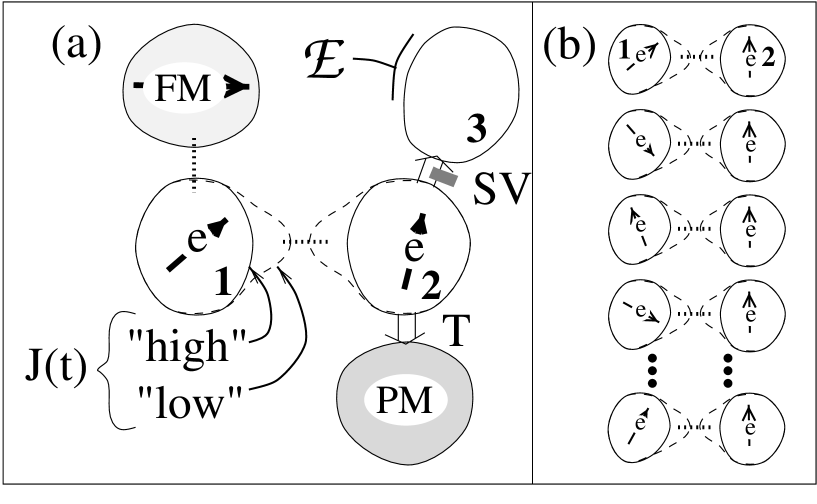
FIG. 1.: a) Schematic top view of two coupled quantum dots labeled 1 and 2, each containing one single excess electron (e) with spin 1/2. The tunnel barrier between the dots can be raised or lowered by setting a gate voltage “high” (solid equipotential contour) or “low” (dashed equipotential contour). In the low state virtual tunneling (dotted line) produces a time-dependent Heisenberg exchange $J(t)$. Hopping to an auxiliary ferromagnetic dot (FM) provides one method of performing single-qubit operations. Tunneling (T) to the paramagnetic dot (PM) can be used as a POV read out with 75% reliability; spin-dependent tunneling (through “spin valve” SV) into dot 3 can lead to spin measurement via an electrometer ${\cal E}$. b) Proposed experimental setup for initial test of swap-gate operation in an array of many non-interacting quantum-dot pairs. Left column of dots is initially unpolarized while right one is polarized; this state can be reversed by a swap operation (see Eq. (40)).

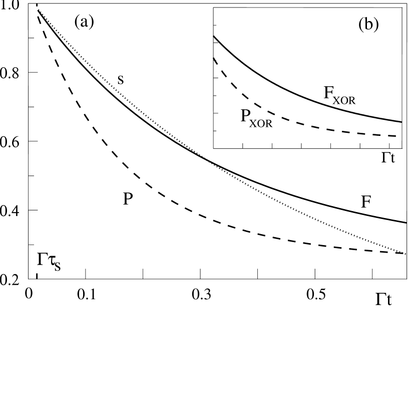
FIG. 2.: a) Swap polarization ${\rm s}\equiv 2\langle S_{1}^{z}(t)\rangle$ (see Eq. (40)), gate fidelity F, and gate purity P vs. $\Gamma t$ for “swap” using parameters $J_{0}\tau_{s}=\pi$, $\Gamma\tau_{s}=0.017$, and $\Delta\tau_{s}=-0.0145$. b) The same for XOR obtained using the four operations in Eq. (2) (the final two single-spin operations done simultaneously). The same parameters and scales as in (a) are used; the pulse-to-pulse time is taken to be $3\tau_{s}$. $\Gamma t$ is measured from the end of the fourth pulse.

REFERENCES

- [1] S. Lloyd, Science 261 1589 (1993); C. H. Bennett, Physics Today 48 (10), 24 (1995); D. P. DiVincenzo, Science 269, 255 (1995); A. Barenco, Contemp. Phys. 37, 375 (1996).
- [2] A. Barenco et al., Phys. Rev. A 52, 3457 (1995).
- [3] P. Shor, Proc. 35th Annual Symposium on the Foundations of Computer Science (IEEE Press, Los Alamitos, 1994) p. 124.
- [4] D. P. DiVincenzo, Report No. cond-mat/9612126, and in Mesoscopic Electron Transport, eds. L. Kouwenhoven, G. Schoen, and L. Sohn, NATO ASI series, to be published.
- [5] J.-I. Cirac and P. Zoller, Phys. Rev. Lett. 74, 4091 (1995); J.-I. Cirac, T. Pellizzari, and P. Zoller, Science 273, 1207 (1996); C. Monroe et al., ibid. 75, 4714 (1995).
- [6] Q. A. Turchette et al., Phys. Rev. Lett. 75, 4710 (1995).
- [7] There has been some earlier speculation on how coupled quantum wells might be used in quantum-scale information processing: see R. Landauer, Science 272, 1914 (1996); A. Barenco et al., Phys. Rev. Lett. 74, 4083 (1995).
- [8] C. Livermore et al., Science 274, 1332 (1996); F. R. Waugh et al., Phys. Rev. B 53, 1413 (1996); F. R. Waugh et al., Phys. Rev. Lett. 75, 705 (1995).
- [9] N. W. Ashcroft and N. D. Mermin, Solid State Physics (Saunders, Philadelphia, 1976), Chap. 32.
- [10] We can also envisage a superexchange mechanism to obtain a Heisenberg interaction by using three aligned quantum dots where the middle one has a higher energy level (by the amount ) such that the electron spins of the outer two dots are also Heisenberg coupled, but now with the exchange coupling being .
- [11] L.I. Glazman and K.A. Matveev, Sov. Phys. JETP 71, 1031 (1990); C.A. Stafford and S. Das Sarma, Phys. Rev. Lett. 72, 3590 (1994).
- [12] We assume for simplicity that the shape of the applied pulse is roughly rectangular with constant.
- [13] We note that explicitly , with the corresponding XOR Hamiltonian, . An alternative way to achieve the XOR operation is given by . This form has the potential advantage that the single qubit operations involve only spin 1.
- [14] A simple discussion of the consequences of decoherence models of this type may be found in I. L. Chuang, R. Laflamme, P. Shor, and W. H. Zurek, Science 270, 1633 (1995).
- [15] For a microscopic discussion of dissipation in quantum dots concerning the charge degrees of freedom see, e.g., H. Schoeller and G. Schön, Phys. Rev. B50, 18436 (1994); Physica B203, 423 (1994).
- [16] E. Fick and G. Sauermann, The Quantum Statistics of Dynamic Processes, Springer Series in Solid-State Sciences 86 (Springer-Verlag, Berlin, 1990).
- [17] E. B. Davies, Quantum Theory of Open Systems, Academic Press, New York (1976).
- [18] M. Celio and D. Loss, Physica A 150, 769 (1989).
- [19] S. A. Crooker et al., Phys. Rev. Lett. 77, 2814 (1996).
- [20] J. F. Poyatos, J.-I. Cirac, and P. Zoller, Phys. Rev. Lett. 78, 390 (1997); Report No. quant-ph/9611013.
- [21] A. Peres, Quantum Theory: Concepts and Methods (Kluwer, Dordrecht, 1993).
- [22] G. Prinz, Physics Today 45 (4), 58 (1995).
- [23] M. Devoret, D. Estève, and Ch. Urbina, Nature 360, 547 (1992).