Lattice Electrons on a Cylinder Surface in the Presence of Rational Magnetic Flux and Disorder[1]

Abstract

We consider a disordered two-dimensional system of independent lattice electrons in a perpendicular magnetic field with rigid confinement in one direction and generalized periodic boundary conditions (GPBC) in the other direction. The objects investigated numerically are the orbits in the plane spanned by the energy eigenvalues and the corresponding center of mass coordinate in the confined direction, parameterized by the phase characterizing the GPBC. The Kubo Hall conductivity is expressed in terms of the winding numbers of these orbits. For vanishing disorder the spectrum of the system consists of Harper bands with energy levels corresponding to the edge states within the band gaps. Disorder leads to broadening of the bands. For sufficiently large systems localized states occur in the band tails. We find that within the mobility gaps of bulk states the Diophantine equation determines the value of the Hall conductivity as known for systems with torus geometry (PBCs in both directions). Within the spectral bands of extended states the Hall conductivity fluctuates strongly. For sufficiently large systems the generic behavior of localization-delocalization transitions characteristic for the quantum Hall effect are recovered.

]

I Introduction

The two-dimensional electron gas in the presence of a strong perpendicular magnetic field provides a rich variety of physical phenomena. The most prominent is the quantum Hall effect [2, 3]. Another fascinating phenomenon is the self-similar energy spectrum (Hofstadter’s butterfly) brought about by a periodic lattice potential and the magnetic field [4, 5]. These phenomena are due to two features originating from the magnetic field: chirality and a characteristic length scale. The chirality is due to the axial vector character of the magnetic field and is responsible for the Hall effect in the presence of an electric field and current carrying edge states in confined systems. The length scale is defined by the size of the cell associated with a single flux quantum and is called the magnetic length. In a periodic potential commensurability effects occur with respect to the ratio of lattice constant and magnetic length. In the presence of disorder also the localization length comes into play which measures the spatial extension of wave functions. The natural way to investigate the interplay of these different length scales is to study the (dissipative and Hall) conductances of multi-terminal systems. Recently, a two-terminal conductance calculation for a clean system was performed by Skjånes et al. [6] and a multi-terminal conductance calculation has been performed by Aldea et al. [7]. For the time being the attempts of calculating directly the multi-terminal conductances of disordered systems are limited by computational practicability. Therefore, in the present paper we restrict ourselves to investigate the energy spectrum, its sensitivity to changing the boundary conditions and the Kubo Hall conductivity.

The system to be studied is a two-dimensional Anderson tight-binding model with Peierls substitution (in Landau gauge) and generalized periodic boundary conditions (GPBC) in one direction and different boundary conditions in the other direction. This system has been investigated by many authors and several results are well established. In the limit of vanishing disorder the Schrödinger equation reduces to a one-dimensional finite difference equation known as Harper’s equation which can be studied effectively by transfer matrix methods. Imposing periodic boundary conditions in both directions corresponds to a torus. If one of these is replaced by rigid wall confinement we are dealing with a cylinder. For both geometries the energy spectrum is periodic in the flux per unit lattice cell (denoted by $\alpha$) with period $1$. Concerning the torus the following results are established: (i) In the case of commensurability, i.e. rational values $\alpha=p/q$ the energy spectrum consists of $q$ Harper bands separated by gaps. The gap structure gives rise to Hofstadter’s butterfly [4]. (ii) The energy spectrum is symmetric with respect to zero energy. (iii) The Hall conductivity is antisymmetric with respect to zero energy (referred to as particle-hole symmetry). (iv) Within the band gaps the Hall conductivity is quantized in integer multiples of $e^{2}/h$; its value is given by a topological quantum number, the first Chern number on the magnetic Brillouin zone. The integer can be determined from the Diophantine equation [8]

$$n=pt_{n}-qs_{n}\,.$$ (1)

Here $t_{n},s_{n}$ are integers corresponding to the $n$-th gap and the Hall conductivity there is $\sigma_{H}=t_{n}(e^{2}/h)$. The solution of Eq. (1) is to be taken under the requirement $|t_{n}|\leq q/2$.

For the cylinder geometry the energy spectrum has also been shown to consist of $q$ Harper bands but the gaps are filled with states localized near the edges in the confined direction ($x$), and extended in the other. These edge states carry a chiral current and give rise to the same quantization of the Hall conductivity as obtained for the torus geometry [9]. Recently [10] an interpretation of the quantization in terms of topological invariants corresponding to these edge states has been proposed and related to the Chern numbers of the torus geometry. However, this relation could be established for no disorder only (see also [11]).

So far, most studies have been focused on the ideal system where analytical results can be obtained (especially the Diophantine equation for the Hall conductivity). It has been argued that disorder will not change the quantized value of the Hall conductivity as long as the disorder does not close the corresponding gap. This is certainly true for the torus geometry where the Hall conductivity is given by the topologically stable Chern number as long as the Fermi energy is within an energy gap. The argument is however not proven for the cylinder geometry where no such gaps exist. Moreover, in the torus geometry disorder leads to levels within the gaps, although the corresponding states are expected to be localized and so do not change the quantization as given by the Diophantine equation. For the torus geometry the following scenario is expected to occur: On increasing the disorder strength localized states appear first in the tails of the disorder broadened Harper bands. When the disorder is further increased the Harper bands begin to overlap strongly and form new bands with possibly less regions of extended states. Yet, for Fermi energies at which a small density of localized states is situated in a previous gap the topological stability of the Chern number still determines the Hall conductivity via the Diophantine equation (cf. Sec. VIII E in[12]).

For the disordered cylinder model (cf. [13, 14]) we cannot rely on the topological stability of Chern numbers when discussing the Hall conductivity. Therefore, in the present work we take a different starting point: we investigate the Hall conductivity in an appropriate version for the cylinder geometry (cf. [15]) and show that in this case also it has a topological meaning as it can be expressed in terms of a winding number. This winding number has an intuitive interpretation: it is the number of oriented windings of those orbits, in a diagram of energy eigenvalues versus the center of mass coordinate, $X$, that connect opposite edge regions. The orbits are parameterized by a continuous quantum number which labels generalized periodic boundary conditions in the direction of current flow ($y$-direction). This winding number is similar to the Chern number when interpreted as the winding number of zeroes of the wavefunction with respect to the change of boundary conditions [16, 17]. We study numerically the influence of increasing disorder on the validity of the Diophantine quantization. We also investigate the Hall conductivity within the Harper bands and show that the Hall conductivity strongly fluctuates as a function of the Fermi energy. For weak disorder and finite system sizes an unexpected collapse of the Hall conductivity occurs in the centers of the bands. This is, however, no surprise when consulting our version of the Kubo Hall conductivity: As long as states in the band centers are extended and do not display large spatial fluctuations, $X$ will be concentrated at the center of the system. Then the Hall conductivity stays close to zero. We expect that as soon as the disorder is strong enough in finite systems or arbitrary small but finite in infinite systems the collapse will disappear and (apart from strong fluctuations) the Hall conductivity effectively interpolates between subsequent the quantized values. The reason for this expectation is that extended states (which in large systems are restricted to the energy band centers) show strong spatial fluctuations which are extremely sensitive to the variation of boundary conditions, i.e. the center coordinate $X$ of such states can be shifted to an arbitrary position within the system by an appropriate change in the boundary conditions. To examine the spatial fluctuations of extended eigenstates and the universal properties of the localization-delocalization transition we calculate the scaling behavior of the distribution of wave function amplitudes of extended states. This (multifractal) analysis (cf. Chap. 12 of [3]) confirms our expectation and, furthermore, we find reasonable agreement with the scaling exponents obtained for other model systems of the integer quantum Hall effect.

The paper is organized as follows: In Sec. II we introduce the model and in Sec. III the methods of calculating energy orbits and the Hall conductivity. The quantization of the Hall conductivity is determined by the topology of the energy orbits. In Sec. IV we present numerical results for the energy orbits corresponding to ideal systems with cylinder geometry and, by comparing to the torus geometry, we demonstrate how edge states appear in the energy gaps of the bulk system. We then turn over to weak disorder and investigate its influence on the topology of energy orbits. The Hall conductivity is unaffected for Fermi energies situated in the bulk energy gaps and is still given by the Diophantine equation, Eq. (1). For Fermi energies situated in the bulk energy bands the Hall conductivity drops down and fluctuates around zero. To see whether this unexpected behavior is still valid for larger systems with strong disorder we present calculations of energy orbits in such systems in Sec. V. We discuss the fluctuation properties of the wave function for extended states in the weak and strong scattering regimes, respectively, and we conclude that for the latter the amplitude fluctuations are strong and display universal characteristics of localization-delocalization transitions in quantum Hall systems. The Hall conductivity interpolates between adjacent plateau values as soon as the system size becomes much larger than the microscopic scales of the model but still exhibits strong mesoscopic fluctuations. Our conclusions are summarized in Sec. VI.

II The model

Consider a two-dimensional (2D) square lattice with lattice constant $a$ and extensions $L_{x}=M_{x}a$, $L_{y}=M_{y}a$. With a set of orthonormal quantum states $\left|{\bf m}\right\rangle$ localized at lattice sites ${\bf m}=(m_{x},m_{y})$ the Hamiltonian of the tight-binding model of independent electrons reads

$$H=\sum_{{\bf m}}\varepsilon_{{\bf m}}\left|{\bf m}\right\rangle\left\langle{\bf m}\right|+\sum_{\left\langle{\bf m},{\bf m}^{\prime}\right\rangle}t_{{\bf m},{\bf m}^{\prime}}\left|{\bf m}\right\rangle\left\langle{\bf m}^{\prime}\right|\,,$$ (2)

where $\left\langle{\bf m},{\bf m}^{\prime}\right\rangle$ denotes nearest neighbors. The site energies $\varepsilon_{{\bf m}}$ correspond to the (random) potential energy and the hopping matrix elements $t_{{\bf m},{\bf m}^{\prime}}$ to the kinetic energy. The magnetic field is included in the kinetic energy by the Peierls substitution

$$t_{{\bf m},{\bf m}^{\prime}}=1\;\;\,\quad\quad\quad\; {\rm if} \;\;m_{y}=m^{\prime}_{y}\;\;{\rm and}\;\;m^{\prime}_{x}=m_{x}\pm 1$$ (3)

$$t_{{\bf m},{\bf m}^{\prime}}=e^{\pm 2\pi i\alpha m_{x}}\;\;\; {\rm if} \;\;m_{x}=m^{\prime}_{x}\;\;{\rm and}\;\;m^{\prime}_{y}=m_{y}\pm 1\,.$$ (4)

Here $\alpha$, restricted to $0<\alpha<1$, is the number of flux quanta $h/e$ per unit cell. The characteristic length associated to $\alpha$ is the magnetic length $l_{B}$ defined by $\alpha=a^{2}/2\pi l_{B}^{2}$. Requiring commensurability between the lattice constant and the magnetic length restricts $\alpha$ to rational values

$$\alpha=p/q\,.$$ (5)

We impose generalized periodic boundary conditions on the eigenfunctions in $y$-direction

$$\psi(m_{x},m_{y}+M_{y})=e^{-2\pi i\vartheta}\psi(m_{x},m_{y})$$ (6)

and Dirichlet boundary conditions in $x$-direction (cylinder)

$$\psi(0,m_{y})=\psi(M_{x}+1,m_{y})=0$$ (7)

or (for comparison) periodic boundary conditions in $x$-direction (torus)

$$\psi(m_{x}+M_{x},m_{y})=\psi(m_{x},m_{y})\,.$$ (8)

The parameter $\vartheta\in[0,1)$ generalizes the periodicity of the wavefunction to be periodic “up to a phase”. $\vartheta/M_{y}$ can, however, also be interpreted as a Bloch quantum number [15]. Indeed, by transforming the eigenvalue problem $H\psi=E\psi$ according to the replacement

$$\psi(m_{x},m_{y})\longrightarrow e^{2\pi i(\vartheta/M_{y})m_{y}}\psi(m_{x},m_{y})$$ (9)

one arrives at an equivalent problem with strictly periodic boundary condition in $y$-direction. The transformed hopping matrix elements read for $m_{x}=m^{\prime}_{x}$, $m_{y}=m^{\prime}_{y}\pm 1$

$$t_{{\bf m},{\bf m}^{\prime}}=e^{\pm 2\pi i[\alpha m_{x}+\vartheta/M_{y}]}\,.$$ (10)

A third way to interpret the parameter is by considering the system as the surface of a cylinder embedded in a 3D space. With $y$ denoting the coordinate along the circumference of the cylinder, $\vartheta$ describes an Aharonov-Bohm flux (in units of the flux quantum) along the cylinder axis (cf. [15]).

III Topology and the Quantum Hall Effect

We adopt the view of considering a family of Hamiltonians $H(\vartheta)$ (characterized by Eqs. (2,3,10)) and wavefunctions that are periodic in $y$-direction. For each member of that family the velocity operator $v_{y}(\vartheta)$ can be obtained by taking the derivative of $H(\vartheta)$ with respect to the Bloch-momentum $\hbar\vartheta/M_{y}$,

$$v_{y}(\vartheta)=\frac{M_{y}}{\hbar}\frac{\partial H(\vartheta)}{\partial\vartheta}\,.$$ (11)

To model a disordered system we take independent random values for the site energies $\varepsilon_{{\bf m}}$ according to a symmetric box distribution on the interval $[-V/2,V/2]$.

For vanishing disorder, $V=0$, and zero magnetic field, $\alpha=0$, the Hamiltonian describes an electron moving in a 2D crystal. The energy band is symmetric around $E=0$ and has the total width $8$. On introducing the rational flux $\alpha=p/q$ and adopting toroidal boundary conditions (Eqs. (6),(8) with $\vartheta=0$) commensurate with the flux lattice, i.e. $M_{x}=ql$ with some integer $l$, the spectrum consists of $q$ magnetic subbands (Harper bands) separated by energy gaps (cf. [4] and Fig. 1 of Ref. [13]) and the statements (i) – (iv) listed in the Introduction apply.

For $V\not=0$ the full 2D problem can be solved by diagonalizing (numerically) the representing (sparse) Hamiltonian matrix which yields the eigenvectors $\psi_{l}({\bf m};\vartheta)$ and eigenvalues $\varepsilon_{l}(\vartheta)$ labeled by the discrete index $l$. In the present work we analyze the model by means of energy orbits to be introduced in the following.

Defining the center of mass coordinate (in $x$-direction) of a given eigenstate by

$$X_{l}(\vartheta):=\sum_{{\bf m}}m_{x}|\psi_{l}({\bf m};\vartheta)|^{2}$$ (12)

allows us to calculate the Hall conductivity $\sigma_{H}=\sigma_{yx}$ by using an appropriate version of the Kubo formula (cf. Eq.(4.76)) in[3]) which, for zero temperature, reads

$$\sigma_{H}=-\frac{e^{2}}{h}\frac{1}{M_{x}}\int\limits_{0}^{1}d\vartheta\,\sum_{l}\Theta\left(\varepsilon_{F}-\varepsilon_{l}(\vartheta)\right)\frac{\partial X_{l}(\vartheta)}{\partial\vartheta}$$ (13)

where $\varepsilon_{F}$ is the Fermi energy. This expression tells that once we know the “energy-orbits” $(X_{l}(\vartheta),\varepsilon_{l}(\vartheta))$ we can read off the Hall conductivity at a given Fermi energy by determining the intersection points, $(X^{(i)},\varepsilon^{(i)}=\varepsilon_{F})$, of the orbits with the line of constant Fermi energy.

$$\sigma_{H}=\sum_{i}\frac{{\rm sign}(i)\,X^{(i)}}{M_{x}}\left(\frac{e^{2}}{h}\right)\,.$$ (14)

This formula tells that one has to add up the center of mass coordinates of the intersection points with a signum $\pm$ depending on crossing from below ($-$) or above ($+$) and finally divides by the width $M_{x}$ resulting in the Hall conductivity (in atomic units). Note that the orbits are (generically) closed, since level crossings occur with zero probability in a disordered system (Wigner-von Neumann theorem [18]).

Those orbits which connect both edge regions of the cylinder are of particular importance: they contribute (almost) integer numbers to the Hall conductivity.

These integer numbers are given by the winding number of orbits connecting both edge regions of the cylinder. The chirality of the orbits defines the sign of the integer, ($+$) for clockwise and ($-$) for counterclockwise windings.

The slight difference between the center of mass coordinate of an edge state $X$ and the geometrical edge ($m_{x}=0,M_{x}$) gives rise to corrections. However, they are of order $(l_{B}/L_{x})$ and furthermore they turn out to be artificially caused by using conductivity instead of conductance (cf. the discussion in [19] and Sec. 4.8 of [3]). In our numerical calculations these corrections are still visible for system sizes of order $100a$. Equation (13) has been analyzed previously in the context of continuous electron systems on the surface of a cylinder [15, 20, 19]. We mention that the very fact of level anti-crossing leads to the presence of energy gaps (mini gaps) in the regime of edge states. Within these mini gaps the Hall conductivity vanishes. A similar observation in a two terminal conductance calculation was denoted in [6] as “cracks in the wings’ of the Hofstadter butterfly. However, these gaps are exponentially small in the ratio of magnetic length vs. system size (cf. [19]) and will be ignored in the following discussions.

We like to comment further on the topological quantization of the Hall conductivity as expressed by the winding numbers of energy orbits. A condition for the occurrence of plateaus in the Hall conductivity is the existence of localized states in the bulk of the system. Such states are characterized by an exponential decay in space far off their center position. The decay length is called the localization length $\xi$. Localized bulk states correspond to orbits degenerated to points since the sensitivity of the center of mass to a change in boundary conditions becomes exponentially weak in the ratio $\xi/L_{x}$. If, for a given Fermi energy, all bulk states of the system are localized but extended edge states do exist, the winding number of these edge states determine the quantized value of the Hall conductivity. This discussion is somewhat simplified since localized bulk states and extended edge states are not degenerate in energy. Rather, the states at a given energy are hybrids of both types of states (see Fig. 9a). As already mentioned in the Introduction the topological quantization in terms of winding numbers is in close analogy to the topological quantization in terms of Chern numbers occurring in the torus geometry. The Chern numbers are given by the winding of the zeroes of wave functions around the torus when two parameters (Bloch quantum numbers) for generalized periodic boundary conditions are changed [16, 17]: Moving the Bloch quantum numbers over their entire Brillouin zone (being also a torus) leads to an integer covering number on the torus in real space. This integer is just the Chern number determining the Hall conductivity. Thus, the Hall conductivity counts the number of times the zeroes of a wave function cover the torus when changing the boundary conditions. In the cylinder geometry the Hall conductivity counts the number of times the center of mass of a wave function covers the cylinder when the boundary conditions are changed. This analogy demonstrates the universality of topological quantization arguments for the Hall conductivity; they are not restricted to a particular geometry although for different geometries the topological quantization can manifest itself in different objects.

A further indication for this universality comes from the observation that the distinction between localized and extended states can be based on topological properties of either model. In the torus geometry localized states are characterized by a vanishing Chern number corresponding to a vanishing covering number for the zeroes of the wave function. In the cylinder geometry localized states are characterized by a vanishing covering number for the center of mass of the wave function. In a quasi-classical treatment (see e.g. [21]) localized states are characterized by closed equipotential lines that do not wind around the cylinder.

Equation (13) not only helps in demonstrating the quantization of the Hall conductivity in a regime of localization but is also suitable for discussing the Hall conductivity in the transition regimes between adjacent plateaus. Here complicated orbits lead to a strongly fluctuating Hall conductivity, as will be discussed in the next sections. It is worth mentioning that similar fluctuations are expected to occur in the torus geometry whenever the Fermi energy crosses a band of extended states (cf. [22]).

A quantity that is simpler than the Hall conductivity and usually still allows to distinguish between localized and extended states is the so-called Thouless number $G$ (cf. [23]) defined as the ratio of a typical energy shift $\delta\varepsilon$ within a band and the average level spacing $\Delta$

$$G=\frac{\delta\varepsilon}{\Delta}$$ (15)

This quantity is similar to a dissipative conductance (in atomic units) since it becomes small compared to $1$ for localized states. However, as we will see, for the cylinder model there are extended edge states even in energy ranges where the bulk states are localized. Thus, the Thouless number will show some non-zero peaks indicating that it is not a suitable criterion for a bulk state to be extended. Therefore we will focus in the following sections on the Hall conductivity, Eq. (13).

IV Weak disorder

We begin our discussion with the limit of vanishing disorder and focus on a significant difference between the torus and the cylinder geometry. As has been pointed out in [9] the difference with respect to the spectrum is that in the cylinder model energy eigenvalues occur in the Harper gaps of the torus model. This can be seen in Fig. 1

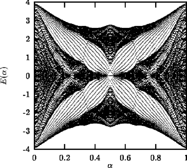
FIG. 1.: Energy spectrum as a function of flux.

where the band structure for the cylinder model is shown as a function of $\alpha$ (the number of flux quanta per unit cell). Regions with dense set of points correspond to the Harper bands while those with lines of points correspond to the gaps (see also Fig. 1 in [4] and Fig. 4 in [9]). For vanishing disorder the translational invariance in $y$-direction yields a wave number $k$ labeling the energy eigenvalues (cf. [4]). The existence of energy branches within the Harper gaps can be easily observed by plotting $\varepsilon_{i}(k)$. In Fig. 2 such plot is shown for $\alpha=1/5$,

FIG. 2.: Energy branches as a function of wave number for flux $\alpha=1/5$.

$\vartheta=0$ and $M_{x}=M_{y}=17$. One observes both the $5$ Harper bands and some energy branches within the Harper gaps. To see that the existence of energy eigenvalues in the Harper gaps is due to edge states it is instructive to plot the energy eigenvalues versus the corresponding center of mass coordinate (in $x$-direction) for a number of $\vartheta$ values. The corresponding plot for the torus geometry is shown in part a) of Fig. 3. This plot not only shows the Harper bands

a)

b)

FIG. 3.: Energy orbits for a system with no disorder and flux $\alpha=1/5$ for a torus geometry (a) and for a cylinder geometry (b).

but also demonstrates that the center of mass, $X$, is distributed within the bulk of the system. For a system with no disorder the wavefunctions are periodic in $x$-direction [24]. Thus, $X$ is distributed within a range smaller than the period. On introducing the cylinder boundary conditions the picture changes. As can be seen in part b) of Fig. 3, the states which have energies within the Harper gaps are concentrated along the edges (see also Fig. 6 of Ref. [6]). Changing $\vartheta$ from $0$ to $1$ can move an edge state from one edge to the opposite edge and, finally, back to the starting point. On the other hand, the states with energies within the Harper bands are less effected by the presence of an edge.

The existence of edge states can be qualitatively understood by considering the Dirichlet boundary conditions together with the chirality inherent in the phase of the hopping elements. For an electron that starts to propagate close to an edge these items lead to a directedness of the most probable path along the edges.

The energy orbits $(\varepsilon_{l}(\vartheta),X_{l}(\vartheta))$ provide a very helpful picture of the spectral properties of the cylinder model and allow to calculate the Hall conductivity rather easily, as discussed after Eq. (13). For example the Hall conductivity for $\alpha=1/5$ is $1,2,-2,-1$ in the first, second, third and fourth gap (from below), respectively. These findings are consistent with the Diophantine equation (1). For values $\alpha=1/q$, with $q$ large, the low lying Harper bands strongly resemble Landau bands of continuous electron models [25] and the quantization of $\sigma_{H}$ in increasing integer steps is no surprise. However, in the lattice model we can take a rational value with a dominator different from $1$, e.g. $\alpha=3/7$. Here the Diophantine equation predicts a sequence of $\sigma_{H}$ as follows: $\sigma_{H}=-2,3,1,-1,-3,2$. As can be seen in Fig. 4 the result is still valid in the cylinder model and coincides with counting the winding numbers of orbits connecting edge states. In fact, in all the cases we analyzed the chirality of the orbits leads to the sign as predicted by the Diophantine equation. Thus, we recover the result obtained in [10] that the Hall conductivity for the cylinder model with vanishing disorder coincides with the Hall conductivity for the torus model with vanishing disorder, as expressed by Eq. (1). The point we wanted to make here was that the concept of winding numbers of energy orbits is suitable to determine the Hall conductivity. We will use this concept further on when increasing successively the strength of disorder.

FIG. 4.: Energy orbits for a cylindrical system with no disorder and flux $\alpha=3/7$.

Let us first consider the case of weak disorder. By this we mean that the disorder strength $V$ is small as compared to the strength of the hopping matrix element ( set $1$). Since for any given matrix size $N$ the number of diagonal elements and the number of non-zero off-diagonal hopping elements are both of order $N$, significant changes in global spectral properties (such as the density of states) occur when $V$ becomes of order $1$. Note, however, that this definition of weak disorder does not apply to disorder related length scales. For example, once the system is large enough localized states will show up in regimes of low density of states. Thus, arbitrarily small amount of disorder can lead to finite localization lengths $\xi$. From this point of view disorder is always strong.

FIG. 5.: Hall conductivity as a function of energy for disorder strength $V=0.9$, flux $\alpha=1/9$ and system size $M=20$.

In the following we will concentrate on a cylinder system with $\alpha=1/9$ and $M_{x}=M_{y}=20$. For $V=0.9$ the Harper bands become broader but still do not overlap. In Fig. 5 the Hall conductivity is shown as a function of the Fermi energy for $V=0.9$. The quantization of $\sigma_{H}$ in the gaps remains valid. However, the behavior of $\sigma_{H}$ within the broadened Harper band is striking: it drops down and fluctuates around zero. A similar behavior can be concluded from the plot of energy orbits for $V=0.6$ displayed in Fig. 6.

FIG. 6.: Energy orbits for disorder strength $V=0.6$, flux $\alpha=1/9$ and system size $M=20$

Again the quantization in the region of bulk states energy gaps according to the Diophantine equation remains valid ($\sigma_{H}=e^{2}/h(1,2,3,-3,-2,-3)$) but the variation of center coordinates $X$ for extended bulk states is restricted to a range of approximately $10$ lattice spacings around the center of the system. Therefore, the Hall conductivity will not exceed the value $0.5$ within the band. The question arises if this behavior will continue for larger systems. If it does, the Hall conductivity will not interpolate between adjacent plateaus but drop down in the transition regimes. To answer this question we first have to understand the origin of the drop in the Hall conductivity. Equation (13) relates the Hall conductivity to the range of center coordinates $X$ for a given energy orbit. For systems of no disorder the amplitude of a wave function is periodic over the flux lattice. Consequently, the range of $X$ is restricted to be less than the period [24]. As soon as we introduce disorder we have to ask about the nature of extended bulk states. It is clear from Eq. (13) that the range of $X$ values can only increase provided the amplitudes of an extended wave function are strongly inhomogeneous. Only then an appropriate shift in the boundary condition parameter $\vartheta$ can lead to a drastic shift in the position $X$ of the center of mass.

The localization length $\xi$ of a wavefunction is the relevant length scale introduced by disorder. It is expected that for sufficiently large system sizes extended states can only exist in the center of the broadened Harper bands. All other bulk states are localized and do not contribute to $\sigma_{H}$. The bulk extended states are characterized by their localization length $\xi$ being larger than the actual system size. In the thermodynamic limit $M=M_{x}=M_{y}\to\infty$ the spectral width of extended bulk states is expected to shrink to zero as $M^{-1/\nu}$ where $\nu$ is the critical exponent of the localization length (cf. [12]). As long as the system size is so small that we hardly find localized states, even in band tails, the system size has to be considered as “microscopic”. The plot of the squared amplitudes (density plot) of two wave functions corresponding to the tail of the first band and to the center of the second band of bulk states are shown in Fig. 7a) and Fig. 7b), respectively. The first state shows a tendency to localize, however the localization length is of the order of the system size. The second state is delocalized and already displays some inhomogeneous amplitude fluctuations. However, for the system size of $M=20$ the center of mass cannot be shifted over the entire scale of $x$-coordinates. Nevertheless, the second state already indicates that the extended bulk states can become spatially inhomogeneous.

a)

b)

FIG. 7.: Density plot of two wave functions with energy in the tail of the first Harper band (a) and within the center of the second Harper band for the same system parameters as in Fig. 6.

V Strong disorder

To see the influence of stronger disorder on the Hall conductivity one can either consider larger systems with fixed disorder strength $V$ or increase the disorder strength $V$. In both cases a reasonable amount of localized states show up in the low density of states regime. We changed the disorder strength and system size for $\alpha=1/9$ to $V=2$ and $M=100$, respectively. The influence of the increased disorder strength can be observed in the density of states which is shown in Fig. 8. The Harper bands strongly overlap and the resolution of only the first and the last Harper gap is possible. These gaps are expected to be filled with localized states and form mobility gaps rather than spectral gaps. We will concentrate on the wave function properties for energies situated within the lowest mobility gap and in the center of the second Harper band.

FIG. 8.: Density of states for flux $\alpha=1/9$ and disorder strength $V=2$ and system size $M=100$.

We find that within the gap all bulk states are now localized and only extended edge states appear, which meets the expectations formulated above. This can be seen in Fig. 9a) where the density plot of a wave function corresponding to a gap energy is displayed. The plot reflects that the wave function has a bulk contribution concentrated on an area with diameter of approximately $16$ lattice spacings and an edge contribution which is extended along one edge in $y$-direction. In contrast to the edge contribution the bulk contribution is almost insensitive to a change in the boundary conditions. For a certain value of the parameter $\vartheta$ the edge contribution will sweep to the opposite edge, resulting in a quantized Hall effect for Fermi energies situated in the mobility gap. The corresponding energy orbits are shown in Fig. 9b) where the movement of edge states can be seen.

a)

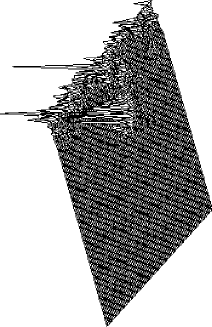
b)

FIG. 9.: Density plot of a wave function with energy in a mobility gap (a) and the corresponding energy orbits (b). The system parameters are the same as in Fig. 8.

The density plot of Fig. 10a) shows a state within the center of the second Harper band. It is a typical example of a critical eigenstate which shows strong spatial amplitude fluctuations. As a consequence the position of its center of mass $X$ can be shifted over a large range of values by an appropriate shift in the parameter $\vartheta$, as seen in Fig. 10b). By this observation we are led to conjecture that the corresponding Hall conductivity will interpolate between adjacent plateau values when increasing further the system size. Still, the Hall conductivity shows strong (mesoscopic) fluctuations of ${\cal O}(e^{2}/h)$ related to the fluctuations of the center of mass coordinate $X$. For this conclusion it is essential that extended bulk states show strong spatial fluctuations. Such fluctuations are a generic feature of electron states at the localization-delocalization transition. In addition, these fluctuations appear on all length scales between microscopic scales and the (diverging) macroscopic localization length and consequently the corresponding density plot represents a multifractal (cf. Chap.12 of [3]). An important feature of critical states is that the typical density, defined as a geometric mean, $P_{\rm typ}=\exp\left\langle\ln|\psi|^{2}\right\rangle$ scales in a universal manner with the system size $M$

$$P_{\rm typ}\propto M^{-\alpha_{0}}$$ (16)

where $\alpha_{0}$ is a critical exponent characteristic of the localization-delocalization transition at hand. The fact that $\alpha_{0}$ is larger than the space dimension indicates the difference between average and typical values of densities and is a criterion for multifractality.

a)

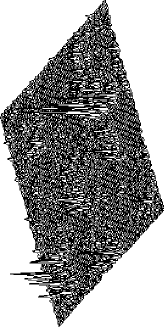
b)

FIG. 10.: Density plot of a wave function with energy in the center of the second Harper band (a) and the corresponding energy orbits (b). The system parameters are the same as in Fig. 9.

In the work by Huckestein et al. [26] the critical eigenstates of the lowest Harper band for $\alpha=1/8$ have been analyzed for a torus geometry. They found the multifractal exponent $\alpha_{0}$ to be consistent with values reported for a number of models related to the quantum Hall effect [27]. A recent calculation [28] yields a value of $\alpha_{0}=2.28\pm 0.02$. For a few of the critical states in the two lowest Harper bands ($\alpha=1/9$, $V=2$, $M=100$) we calculated the exponent $\alpha_{0}$ and found values of $\alpha_{0}$ compatible with those reported previously. This indicates that in the center of the Harper bands localization-delocalization transitions occur in accordance with the quantum Hall universality class.

VI Conclusion

We presented numerical calculations of energy eigenvalues and wave functions for disordered lattice electron systems on a cylinder surface in the presence of rational magnetic flux. We analyzed the Hall conductivity by means of closed orbits in the energy vs. center of mass plane. The orbits are parameterized by an Aharonov-Bohm flux along the cylinder axis. The spectrum is found to consist of disorder broadened Harper bands with Harper gaps filled by localized bulk states and/or delocalized edge states. In the regime of these bulk mobility gaps the Hall conductivity is quantized and given by the Diophantine equation, Eq. (1), originally derived for clean systems with torus geometry.

In close analogy to systems with torus geometry the quantized Hall conductivity for systems with cylinder geometry is shown to be related to topological quantum numbers. Whereas for the torus these are Chern numbers, they are the winding numbers of the above defined orbits in the case of the cylinder. Thus, concerning the often discussed “topological explanation” of the quantum Hall effect both geometries are shown to be essentially equivalent.

Within the broadened Harper bands a regime of extended bulk states exist. Regarding the drop in the Hall conductivity for very small and weakly disordered systems, we do not expect that this drop will occur in a real multi-terminal measurement. Let us stress that the Hall conductivity assumes a uniform electric field within the system while a true conductance must be based on the self-consistent field within the system. As discussed in Ref. [3] the difference between conductance and conductivity is negligeble (${\cal O}(l_{B}/L)$) for discussing the plateau region, however this is not the case in the region of bulk-extended states. These bulk states are, for sufficiently large enough systems, multifractal with universal characteristics of critical states in quantum Hall systems. The multifractality is directly connected to the mesoscopic fluctuations of the Hall conductivity within the regime of critical states; the sensitivity of the center of mass to the Aharonov-Bohm flux leads to drastic fluctuations of the Hall conductivity. These fluctuations are of order $e^{2}/h$ and the distribution of the Hall conductivity in the transition regime between Hall plateaus deserves further studies. Although the very fact of mesoscopic fluctuations in the conductivity points to a similar effect for the conductance, a direct quantitative comparison is not possible. The work by Aldea et al. [7], where multi-terminal conductances were calculated (for systems of $\approx 600$ lattice sites), gives support to the expectation that a true multi-terminal Hall conductance fluctuates between subsequent plateaus. The experimentally observed flat distribution [29] of two-terminal conductances in the transition regime is compatible with the fluctuations we found in our calculations of the Hall conductivity. They have been reproduced for the two-terminal conductance within a (one Landau band) network model of a quantum Hall system [30]. In our model similar fluctuations correspond to the strong amplitude fluctuations in critical (multifractal) eigenstates.

Acknowledgment

This work was performed within the research program of the Sonderforschungsbereich 341 of the Deutsche Forschungsgemeinschaft.

REFERENCES

- [1] Dedicated to Professor Wolfgang Götze on the occasion of his 60th birthday
- [2] R.E. Prange, S. Girvin (Eds.), The Quantum Hall Effect, Springer, New York (1990).
- [3] M. Janssen, O. Viehweger, U. Fastenrath, J. Hajdu, Introduction to the Theory of the Integer Quantum Hall Effect, VCH, Weinheim (1994).
- [4] D.R. Hofstadter, Phys. Rev. B14, 2239 (1976).
- [5] T. Schloesser, K. Ensslin, J.P. Kotthaus, M. Holland, Europhys. Lett. 33, 683 (1996).
- [6] J. Skjånes, E.H. Hauge, G. Schön, Phys. Rev. B50, 8636 (1994).
- [7] A. Aldea, P. Gartner, A. Manolescu, M. Nita, unpublished (1996).
- [8] D.J. Thouless, M. Kohmoto, M.P. Nightingale, M. den Nijs, Phys. Rev. Lett. 49, 405 (1982).
- [9] R. Rammal, G. Toulouse, M. T. Jaekel, B. I. Halperin, Phys. Rev. B 27, 5142 (1983).
- [10] Y. Hatsugai, Phys. Rev. B48, 11851 (1993); Phys. Rev. Lett. 71, 3697 (1993).
- [11] P. Středa, J. Kučera, D. Pfannkuche, R.R. Gerhardts, A.H. MacDonald, Phys. Rev. B 50, 11955 (1994).
- [12] B. Huckestein, Rev. Mod. Phys. 67, 357 (1995).
- [13] L. Schweitzer, B. Kramer, A. MacKinnon, J. Phys. C 17, 4111 (1984).
- [14] H. Aoki, J. Phys. C18, L67 (1984).
- [15] J. Hajdu, M. Janssen, O. Viehweger, Z. Phys. B66, 433 (1987).
- [16] M. Kohmoto, Ann. Phys. (N.Y.) 160, 343 (1985).
- [17] D. P. Arovas, R. N. Bhatt, F. D. M. Haldane, P. B. Littlewood, R. Rammal, Phys. Rev. Lett. 60, 619 (1988).
- [18] E. Wigner, J. von Neumann, Z. Phys. 30, 467 (1929).
- [19] O. Viehweger, W. Pook, M. Janßen, J. Hajdu, Z. Phys. B 78, 11 (1990).
- [20] T. Ohtsuki, Y. Ono, Solid State Commun. 65, 403 (1988).
- [21] S. M. Apenko, Y. E. Lozovik, Sov. Phys. JETP 62(2), 328 (1985).
- [22] W. Pook, J. Hajdu, Z. Phys. B 66, 427 (1987).
- [23] D. J. Thouless, Phys. Rep. 13 C, 93 (1974).
- [24] The period is typically equal to . Due to degeneracies larger periods equal to an integer multiple of can occur.
- [25] V. Gudmundsson, R.R. Gerhardts, R. Johnston, L. Schweitzer, Z. Phys. B70, 453 (1988).
- [26] B. Huckestein, B. Kramer, L. Schweitzer, Surface Sciences 263, 125 (1992).
- [27] W. Pook, M. Janssen, Z. Phys. B 82, 295 (1991); R. Klesse, M. Metzler, Europhys. Lett. 32, 229 (1995).
- [28] P. Freche, unpublished (1996).
- [29] D. H. Cobden, E. Kogan, unpublished, cond-mat/9606114 (1996).
- [30] S. Cho, P. A. Fisher, unpublished, cond-mat/9609048 (1996).